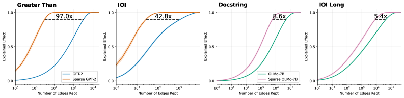
## Chart: Explained Effect vs. Number of Edges Kept for Different Models and Tasks ### Overview The image presents four line charts comparing the "Explained Effect" as a function of the "Number of Edges Kept" for different models (GPT-2 and OLMo-7B) and tasks ("Greater Than", "IOI", "Docstring", and "IOI Long"). Each chart compares a standard model with its sparse counterpart. The x-axis (Number of Edges Kept) is on a logarithmic scale. The charts show how well the models perform as the number of edges is reduced. ### Components/Axes * **Titles (Top of each chart):** * Chart 1: "Greater Than" * Chart 2: "IOI" * Chart 3: "Docstring" * Chart 4: "IOI Long" * **Y-axis (Shared):** * Label: "Explained Effect" * Scale: 0.0 to 1.0, with tick marks at 0.0 and 0.5. * **X-axis (Shared):** * Label: "Number of Edges Kept" * Scale: Logarithmic, ranging from 10^0 to 10^4 (Charts 1 & 2) and 10^0 to 10^5 (Charts 3 & 4). * **Legends (Bottom-left of each chart):** * Chart 1 & 2: * Blue line: "GPT-2" * Orange line: "Sparse GPT-2" * Chart 3 & 4: * Green line: "OLMo-7B" * Pink line: "Sparse OLMo-7B" * **Annotations:** Each chart has an annotation indicating the "x" factor, representing the ratio of edges kept between the dense and sparse models at the point where the explained effect plateaus. ### Detailed Analysis **Chart 1: Greater Than** * **GPT-2 (Blue):** The explained effect increases slowly from 0 to 1 as the number of edges kept increases from 10^0 to approximately 10^3. * At 10^0 edges, the explained effect is approximately 0.1. * At 10^1 edges, the explained effect is approximately 0.2. * At 10^2 edges, the explained effect is approximately 0.6. * At 10^3 edges, the explained effect is approximately 0.95. * At 10^4 edges, the explained effect is approximately 1.0. * **Sparse GPT-2 (Orange):** The explained effect increases rapidly from approximately 0.2 to 1 as the number of edges kept increases from 10^0 to approximately 10^2. * At 10^0 edges, the explained effect is approximately 0.2. * At 10^1 edges, the explained effect is approximately 0.9. * At 10^2 edges, the explained effect is approximately 1.0. * **Annotation:** "97.0x" is displayed above a dashed horizontal line at an explained effect of approximately 0.92. **Chart 2: IOI** * **GPT-2 (Blue):** The explained effect increases slowly from approximately 0.1 to 1 as the number of edges kept increases from 10^0 to approximately 10^3. * At 10^0 edges, the explained effect is approximately 0.1. * At 10^1 edges, the explained effect is approximately 0.3. * At 10^2 edges, the explained effect is approximately 0.8. * At 10^3 edges, the explained effect is approximately 0.95. * At 10^4 edges, the explained effect is approximately 1.0. * **Sparse GPT-2 (Orange):** The explained effect increases rapidly from approximately 0.3 to 1 as the number of edges kept increases from 10^0 to approximately 10^2. * At 10^0 edges, the explained effect is approximately 0.3. * At 10^1 edges, the explained effect is approximately 0.8. * At 10^2 edges, the explained effect is approximately 1.0. * **Annotation:** "42.8x" is displayed above a dashed horizontal line at an explained effect of approximately 0.92. **Chart 3: Docstring** * **OLMo-7B (Green):** The explained effect increases slowly from approximately 0 to 1 as the number of edges kept increases from 10^0 to approximately 10^5. * At 10^0 edges, the explained effect is approximately 0.0. * At 10^1 edges, the explained effect is approximately 0.02. * At 10^2 edges, the explained effect is approximately 0.05. * At 10^3 edges, the explained effect is approximately 0.15. * At 10^4 edges, the explained effect is approximately 0.6. * At 10^5 edges, the explained effect is approximately 0.95. * **Sparse OLMo-7B (Pink):** The explained effect increases rapidly from approximately 0 to 1 as the number of edges kept increases from 10^0 to approximately 10^4. * At 10^0 edges, the explained effect is approximately 0.0. * At 10^1 edges, the explained effect is approximately 0.05. * At 10^2 edges, the explained effect is approximately 0.1. * At 10^3 edges, the explained effect is approximately 0.3. * At 10^4 edges, the explained effect is approximately 0.9. * At 10^5 edges, the explained effect is approximately 1.0. * **Annotation:** "8.6x" is displayed above a dashed horizontal line at an explained effect of approximately 0.92. **Chart 4: IOI Long** * **OLMo-7B (Green):** The explained effect increases slowly from approximately 0 to 1 as the number of edges kept increases from 10^0 to approximately 10^5. * At 10^0 edges, the explained effect is approximately 0.0. * At 10^1 edges, the explained effect is approximately 0.05. * At 10^2 edges, the explained effect is approximately 0.1. * At 10^3 edges, the explained effect is approximately 0.2. * At 10^4 edges, the explained effect is approximately 0.6. * At 10^5 edges, the explained effect is approximately 0.95. * **Sparse OLMo-7B (Pink):** The explained effect increases rapidly from approximately 0 to 1 as the number of edges kept increases from 10^0 to approximately 10^4. * At 10^0 edges, the explained effect is approximately 0.0. * At 10^1 edges, the explained effect is approximately 0.1. * At 10^2 edges, the explained effect is approximately 0.2. * At 10^3 edges, the explained effect is approximately 0.4. * At 10^4 edges, the explained effect is approximately 0.8. * At 10^5 edges, the explained effect is approximately 1.0. * **Annotation:** "5.4x" is displayed above a dashed horizontal line at an explained effect of approximately 0.92. ### Key Observations * In all four charts, the sparse models (Sparse GPT-2, Sparse OLMo-7B) achieve a similar "Explained Effect" to their dense counterparts (GPT-2, OLMo-7B) with significantly fewer edges. * The "x" factor annotations indicate the ratio of edges required by the dense model compared to the sparse model to achieve a similar level of "Explained Effect". * The "Greater Than" task shows the largest difference between the dense and sparse models (97.0x), while "IOI Long" shows the smallest difference (5.4x). ### Interpretation The charts demonstrate that sparse models can achieve comparable performance to dense models while using significantly fewer parameters (edges). This suggests that many connections in dense models are redundant and can be pruned without significantly impacting performance. The "x" factor annotations quantify the degree of redundancy for each task. The "Greater Than" task appears to be the most amenable to sparsification, while "IOI Long" is the least. This could be due to the inherent complexity of each task and the specific architecture of the models. The data suggests that sparse models are a promising approach for reducing the computational cost and memory footprint of large language models.

## Line Charts: Explained Effect vs. Number of Edges Kept Across Four Tasks ### Overview The image consists of a 1x4 grid of line charts comparing the performance of standard language models against their "Sparse" counterparts across four different tasks: "Greater Than", "IOI", "Docstring", and "IOI Long". The charts illustrate how rapidly each model achieves a high "Explained Effect" as the "Number of Edges Kept" increases. In all four panels, the sparse models achieve higher explained effects with significantly fewer edges than the standard models. ### Components/Axes All four charts share identical axis definitions and scales: * **Y-Axis:** Labeled "Explained Effect". The scale is linear, with major tick marks and gridlines at **0.0, 0.5, and 1.0**. * **X-Axis:** Labeled "Number of Edges Kept". The scale is logarithmic (base 10). The range varies slightly depending on the model being evaluated: * Charts 1 & 2 (GPT-2): Ticks at **$10^0$, $10^1$, $10^2$, $10^3$, $10^4$**. * Charts 3 & 4 (OLMo-7B): Ticks at **$10^0$, $10^1$, $10^2$, $10^3$, $10^4$, $10^5$**. * **Legends:** * Located in the bottom-right corner of the first chart ("Greater Than"): * **Blue Line:** GPT-2 * **Orange Line:** Sparse GPT-2 * *(Note: This color coding applies to the second chart, "IOI", as well).* * Located in the bottom-right corner of the third chart ("Docstring"): * **Green Line:** OLMo-7B * **Pink/Purple Line:** Sparse OLMo-7B * *(Note: This color coding applies to the fourth chart, "IOI Long", as well).* * **Annotations:** Each chart features a horizontal dashed black line connecting the two curves at approximately the y = 0.9 level. Above this dashed line is a text label indicating a multiplier (e.g., "97.0x"), representing the ratio of edges required by the standard model versus the sparse model to achieve that specific Explained Effect. ### Detailed Analysis #### Panel 1: Greater Than (Far Left) * **Trend Verification:** The orange line (Sparse GPT-2) rises sharply from the y-intercept, reaching maximum effect quickly. The blue line (GPT-2) remains low initially and requires a much higher number of edges to rise. * **Data Points (Approximate):** * **Sparse GPT-2 (Orange):** Starts at y ~ 0.15 (x=$10^0$). Reaches y=0.5 at x ~ $10^1$. Reaches y=0.9 at x ~ 30. Reaches y=1.0 just after x=$10^2$. * **GPT-2 (Blue):** Starts at y ~ 0.0 (x=$10^0$). Reaches y=0.5 at x ~ $10^3$. Reaches y=0.9 at x ~ 3,000. Reaches y=1.0 near x=$10^4$. * **Annotation:** A dashed line at y ~ 0.9 connects the curves. The label reads **97.0x**, indicating GPT-2 requires 97 times more edges than Sparse GPT-2 to reach this level of explained effect. #### Panel 2: IOI (Center Left) * **Trend Verification:** Similar to Panel 1, the orange line (Sparse GPT-2) ascends much faster than the blue line (GPT-2). * **Data Points (Approximate):** * **Sparse GPT-2 (Orange):** Starts at y ~ 0.25 (x=$10^0$). Reaches y=0.5 at x ~ 5. Reaches y=0.9 at x ~ 40. Reaches y=1.0 near x=$10^2$. * **GPT-2 (Blue):** Starts at y ~ 0.05 (x=$10^0$). Reaches y=0.5 at x ~ $10^2$. Reaches y=0.9 at x ~ 1,700. Reaches y=1.0 near x=$10^4$. * **Annotation:** A dashed line at y ~ 0.9 connects the curves. The label reads **42.8x**. #### Panel 3: Docstring (Center Right) * **Trend Verification:** The pink line (Sparse OLMo-7B) rises steadily, preceding the green line (OLMo-7B), which follows a similar but delayed trajectory along the x-axis. * **Data Points (Approximate):** * **Sparse OLMo-7B (Pink):** Starts at y ~ 0.0 (x=$10^0$). Reaches y=0.5 at x ~ $10^3$. Reaches y=0.9 at x ~ 4,000. Reaches y=1.0 near x=$10^4$. * **OLMo-7B (Green):** Starts at y ~ 0.0 (x=$10^0$). Reaches y=0.5 at x ~ $10^4$. Reaches y=0.9 at x ~ 35,000. Reaches y=1.0 near x=$10^5$. * **Annotation:** A dashed line at y ~ 0.9 connects the curves. The label reads **8.6x**. #### Panel 4: IOI Long (Far Right) * **Trend Verification:** The pink line (Sparse OLMo-7B) rises before the green line (OLMo-7B), though the gap between them appears visually narrower than in the GPT-2 charts. * **Data Points (Approximate):** * **Sparse OLMo-7B (Pink):** Starts at y ~ 0.0 (x=$10^0$). Reaches y=0.5 at x ~ 500. Reaches y=0.9 at x ~ 10,000. Reaches y=1.0 near x=$10^5$. * **OLMo-7B (Green):** Starts at y ~ 0.0 (x=$10^0$). Reaches y=0.5 at x ~ 3,000. Reaches y=0.9 at x ~ 54,000. Reaches y=1.0 slightly after the pink line. * **Annotation:** A dashed line at y ~ 0.9 connects the curves. The label reads **5.4x**. ### Key Observations 1. **Consistent Superiority of Sparse Models:** In every task evaluated, the "Sparse" version of the model (Sparse GPT-2, Sparse OLMo-7B) achieves a high "Explained Effect" using orders of magnitude fewer "Edges" than the baseline models. 2. **Varying Efficiency Gains:** The efficiency multiplier (annotated at the ~0.9 Explained Effect mark) varies drastically depending on the model and task. The gain is massive for GPT-2 on the "Greater Than" task (97.0x) but much more modest for OLMo-7B on the "IOI Long" task (5.4x). 3. **Model Scale Differences:** The x-axis reveals that the OLMo-7B models generally require more edges overall (up to $10^5$) to reach a 1.0 explained effect compared to the GPT-2 models (which max out around $10^4$), reflecting the likely difference in the total size and complexity of the underlying models. ### Interpretation These charts are highly indicative of research in **mechanistic interpretability** or **network pruning** within Large Language Models (LLMs). * **"Edges Kept"** likely refers to the connections between nodes, attention heads, or MLP layers within the neural network's computational graph (often referred to as a "circuit"). * **"Explained Effect"** represents how well a sub-network (the kept edges) can replicate the performance or specific behavior of the full, unpruned model on a specific task (like "Greater Than" or "Indirect Object Identification - IOI"). **The core finding demonstrated by this data is that "Sparse" models are vastly more efficient for circuit discovery.** The data proves that by using a sparse variant of a model, researchers can isolate the specific pathways (edges) responsible for a task while throwing away the vast majority of the network. For example, in the "Greater Than" task, the sparse GPT-2 model can explain ~90% of the model's behavior using nearly 100 times fewer connections than standard GPT-2. This suggests that the sparse models have highly localized, disentangled representations for these tasks, making them significantly easier to interpret and analyze than their dense counterparts.

\n ## Charts: Sparsity vs. Explained Effect ### Overview The image presents four charts comparing the "Explained Effect" of different models (GPT-2, OLMo-7B) and their sparse counterparts as a function of the "Number of Edges Kept". Each chart focuses on a different evaluation context: "Greater Than", "IOI", "Docstring", and "IOI Long". The charts visually demonstrate how much of the effect is explained as the number of edges retained in the model increases. ### Components/Axes Each chart shares the following components: * **X-axis:** "Number of Edges Kept" - Logarithmic scale from 10⁰ to 10⁵. * **Y-axis:** "Explained Effect" - Linear scale from 0.0 to 1.0. * **Title:** Indicates the evaluation context ("Greater Than", "IOI", "Docstring", "IOI Long"). * **Legend:** Identifies the data series. The four charts have the following specific data series: 1. **"Greater Than" Chart:** * GPT-2 (Orange) * Sparse GPT-2 (Blue) 2. **"IOI" Chart:** * GPT-2 (Orange) * Sparse GPT-2 (Blue) 3. **"Docstring" Chart:** * OLMo-7B (Pink) * Sparse OLMo-7B (Green) 4. **"IOI Long" Chart:** * OLMo-7B (Pink) * Sparse OLMo-7B (Green) Each chart also includes a dashed horizontal line with a numerical value indicating the relative improvement of the sparse model over the dense model. ### Detailed Analysis **1. "Greater Than" Chart:** * **GPT-2 (Orange):** The line starts at approximately 0.05 at 10⁰ edges and rapidly increases, reaching approximately 0.95 at 10³ edges. It plateaus around 0.98 after 10³ edges. * **Sparse GPT-2 (Blue):** The line starts at approximately 0.05 at 10⁰ edges and increases more slowly than GPT-2, reaching approximately 0.85 at 10³ edges. It plateaus around 0.95 after 10³ edges. * **Improvement:** The dashed line indicates a 97.0x improvement. **2. "IOI" Chart:** * **GPT-2 (Orange):** The line starts at approximately 0.05 at 10⁰ edges and rapidly increases, reaching approximately 0.95 at 10³ edges. It plateaus around 0.99 after 10³ edges. * **Sparse GPT-2 (Blue):** The line starts at approximately 0.05 at 10⁰ edges and increases more slowly than GPT-2, reaching approximately 0.80 at 10³ edges. It plateaus around 0.95 after 10³ edges. * **Improvement:** The dashed line indicates a 42.8x improvement. **3. "Docstring" Chart:** * **OLMo-7B (Pink):** The line starts at approximately 0.1 at 10⁰ edges and increases, reaching approximately 0.75 at 10³ edges. It plateaus around 0.90 after 10³ edges. * **Sparse OLMo-7B (Green):** The line starts at approximately 0.1 at 10⁰ edges and rapidly increases, reaching approximately 0.95 at 10³ edges. It plateaus around 0.99 after 10³ edges. * **Improvement:** The dashed line indicates a 8.6x improvement. **4. "IOI Long" Chart:** * **OLMo-7B (Pink):** The line starts at approximately 0.1 at 10⁰ edges and increases, reaching approximately 0.70 at 10³ edges. It plateaus around 0.85 after 10³ edges. * **Sparse OLMo-7B (Green):** The line starts at approximately 0.1 at 10⁰ edges and rapidly increases, reaching approximately 0.90 at 10³ edges. It plateaus around 0.98 after 10³ edges. * **Improvement:** The dashed line indicates a 5.4x improvement. ### Key Observations * In all four charts, the sparse models (Blue/Green) consistently show a slower initial increase in "Explained Effect" compared to their dense counterparts (Orange/Pink). * However, the sparse models eventually reach comparable or even slightly higher levels of "Explained Effect" with fewer edges. * The magnitude of improvement varies significantly across the evaluation contexts. "Greater Than" shows the largest improvement (97.0x), while "IOI Long" shows the smallest (5.4x). * The "IOI" chart shows a very high explained effect for the dense GPT-2 model, reaching nearly 1.0 with a relatively small number of edges. ### Interpretation These charts demonstrate the benefits of sparsity in large language models. While dense models initially achieve higher "Explained Effect" with a small number of edges, sparse models can achieve comparable or better performance with significantly fewer parameters (edges). This suggests that sparsity can be an effective technique for model compression and efficiency without sacrificing performance. The varying degrees of improvement across different evaluation contexts suggest that the effectiveness of sparsity depends on the specific task or data distribution. The "Greater Than" context, for example, may be more amenable to sparsity than the "IOI Long" context. The horizontal lines representing the improvement factor provide a quantitative measure of the benefits of sparsity. A higher improvement factor indicates a greater reduction in the number of parameters required to achieve a given level of performance. The fact that all improvement factors are greater than 1 indicates that sparsity is generally beneficial in these scenarios. The charts highlight a trade-off between initial performance and long-term efficiency. Dense models may be faster to train and achieve higher initial performance, but sparse models offer the potential for significant long-term savings in terms of storage and computational cost.

## Comparative Analysis of Sparse vs. Dense Model Efficiency ### Overview The image displays a 1x4 grid of line charts comparing the performance of standard ("dense") neural network models against their "sparse" counterparts. Each chart plots the "Explained Effect" (y-axis) against the "Number of Edges Kept" (x-axis, logarithmic scale). The central finding is that sparse models achieve the same level of explained effect with significantly fewer parameters (edges), with the efficiency gain (multiplier) varying by task. ### Components/Axes * **Chart Type:** 4 separate line charts arranged horizontally. * **X-Axis (All Charts):** "Number of Edges Kept". Scale is logarithmic (base 10). * Charts 1 & 2 ("Greater Than", "IOI"): Range from 10⁰ (1) to 10⁴ (10,000). * Charts 3 & 4 ("Docstring", "IOI Long"): Range from 10¹ (10) to 10⁵ (100,000). * **Y-Axis (All Charts):** "Explained Effect". Linear scale from 0.0 to 1.0. * **Legends:** Located in the bottom-right corner of each subplot. * Chart 1: Blue line = "GPT-2", Orange line = "Sparse GPT-2" * Chart 2: Blue line = "GPT-2", Orange line = "Sparse GPT-2" * Chart 3: Green line = "OLMo-7B", Pink line = "Sparse OLMo-7B" * Chart 4: Green line = "OLMo-7B", Pink line = "Sparse OLMo-7B" * **Annotations:** Each chart contains a dashed horizontal line near the top (y ≈ 0.95-0.98) with a multiplier value (e.g., "97.0x") indicating the relative efficiency of the sparse model. ### Detailed Analysis **Chart 1: "Greater Than"** * **Trend Verification:** The orange "Sparse GPT-2" curve rises steeply from the left, reaching near-maximum explained effect (~0.95) at approximately 10² edges. The blue "GPT-2" curve rises much more gradually, reaching the same effect level at nearly 10⁴ edges. * **Key Data Point/Annotation:** "97.0x". This indicates the sparse model requires roughly 97 times fewer edges to achieve the same high explained effect as the dense model on this task. * **Spatial Grounding:** The dashed line and "97.0x" label are positioned in the upper center of the plot area. **Chart 2: "IOI"** * **Trend Verification:** Similar pattern to Chart 1. The orange "Sparse GPT-2" curve is significantly to the left of the blue "GPT-2" curve, indicating superior parameter efficiency. * **Key Data Point/Annotation:** "42.8x". The efficiency gain is substantial but less extreme than for the "Greater Than" task. * **Spatial Grounding:** Annotation is centered in the upper plot area. **Chart 3: "Docstring"** * **Trend Verification:** The pink "Sparse OLMo-7B" curve is to the left of the green "OLMo-7B" curve, but the gap between them is narrower than in the first two charts. Both curves have a sigmoidal shape. * **Key Data Point/Annotation:** "8.6x". The sparse model is still more efficient, but the advantage is an order of magnitude smaller than for the GPT-2 models on the previous tasks. * **Spatial Grounding:** Annotation is centered in the upper plot area. **Chart 4: "IOI Long"** * **Trend Verification:** The pink "Sparse OLMo-7B" curve is again to the left of the green "OLMo-7B" curve. The curves are closer together than in Chart 3. * **Key Data Point/Annotation:** "5.4x". This represents the smallest efficiency multiplier among the four charts. * **Spatial Grounding:** Annotation is centered in the upper plot area. ### Key Observations 1. **Universal Efficiency Gain:** In all four tasks, the sparse model variant achieves any given level of "Explained Effect" with fewer edges than its dense counterpart. 2. **Diminishing Multiplier:** The efficiency multiplier decreases dramatically across the charts: 97.0x → 42.8x → 8.6x → 5.4x. 3. **Task/Model Dependency:** The magnitude of the sparsification benefit is highly dependent on both the model architecture (GPT-2 vs. OLMo-7B) and the specific task ("Greater Than" vs. "IOI" vs. "Docstring" vs. "IOI Long"). 4. **Curve Shape:** All curves are sigmoidal (S-shaped), indicating a phase transition where explanatory power rapidly increases after a certain threshold of edges is retained. ### Interpretation This data provides strong empirical evidence for the **pruning hypothesis** in neural networks: that a significant portion of a model's parameters (edges) are redundant for specific tasks. The "Explained Effect" likely measures how well a subnetwork (defined by the kept edges) can replicate the full model's behavior or performance. The key insight is that **the degree of redundancy is not constant**. The massive 97x multiplier for "Greater Than" suggests this is a relatively simple, localized computation that can be encoded in a very small sub-circuit of GPT-2. In contrast, the "IOI Long" task (likely a more complex, long-range dependency problem) shows less redundancy (5.4x), implying its solution is more distributed across the network's parameters. The transition from GPT-2 to the larger OLMo-7B model, and from simpler to more complex tasks, shows a clear trend: **as task complexity and/or model scale increases, the relative efficiency gain from sparsification decreases, though it remains positive.** This has profound implications for model compression and efficient AI, suggesting that while pruning is universally beneficial, its most dramatic savings are found in simpler cognitive tasks or within smaller models. The consistent sigmoidal curves further suggest there exists a critical minimal subnetwork size required to solve a task, below which performance collapses.

## Line Graphs: Explained Effect vs. Number of Edges Kept ### Overview The image contains four line graphs arranged in a 2x2 grid, comparing the performance of sparse vs. non-sparse models across different tasks. Each graph plots "Explained Effect" (y-axis, 0.0–1.0) against "Number of Edges Kept" (x-axis, logarithmic scale: 10⁰ to 10⁵). The graphs are labeled "Greater Than," "IOI," "Docstring," and "IOI Long," with distinct color-coded lines for each model variant. ### Components/Axes - **X-axis**: "Number of Edges Kept" (logarithmic scale: 10⁰, 10¹, 10², 10³, 10⁴, 10⁵). - **Y-axis**: "Explained Effect" (linear scale: 0.0 to 1.0). - **Legends**: - **Top-left graphs ("Greater Than," "IOI")**: - Blue line: "GPT-2" (non-sparse). - Orange line: "Sparse GPT-2" (sparse). - **Bottom-right graphs ("Docstring," "IOI Long")**: - Teal line: "OLMo-7B" (non-sparse). - Pink line: "Sparse OLMo-7B" (sparse). - **Annotations**: Multipliers (e.g., "97.0x," "42.8x") indicate efficiency gains of sparse models over non-sparse baselines. ### Detailed Analysis 1. **Greater Than** - **Sparse GPT-2 (orange)**: Rapidly plateaus near 1.0 at ~10² edges, annotated with "97.0x" efficiency gain. - **GPT-2 (blue)**: Gradually approaches 1.0, requiring ~10³ edges. 2. **IOI** - **Sparse GPT-2 (orange)**: Plateaus near 1.0 at ~10² edges, annotated with "42.8x" efficiency gain. - **GPT-2 (blue)**: Reaches 1.0 at ~10³ edges. 3. **Docstring** - **Sparse OLMo-7B (pink)**: Plateaus near 1.0 at ~10³ edges, annotated with "8.6x" efficiency gain. - **OLMo-7B (teal)**: Reaches 1.0 at ~10⁴ edges. 4. **IOI Long** - **Sparse OLMo-7B (pink)**: Plateaus near 1.0 at ~10⁴ edges, annotated with "5.4x" efficiency gain. - **OLMo-7B (teal)**: Reaches 1.0 at ~10⁵ edges. ### Key Observations - **Efficiency Gains**: Sparse models achieve near-maximum explained effect with significantly fewer edges than non-sparse models (e.g., 97.0x faster in "Greater Than"). - **Diminishing Returns**: Non-sparse models show gradual improvement, while sparse models plateau early, suggesting limited benefit from additional edges. - **Task-Specific Performance**: Efficiency gains vary by task (e.g., "Greater Than" has the highest multiplier at 97.0x). ### Interpretation The data demonstrates that sparse models (e.g., Sparse GPT-2, Sparse OLMo-7B) drastically reduce computational requirements while maintaining high performance, as evidenced by their early plateaus and high efficiency multipliers. This suggests sparse architectures are optimal for resource-constrained environments. The diminishing returns for non-sparse models highlight the importance of edge selection in model efficiency. The task-specific multipliers indicate that sparsity benefits vary depending on the problem domain.