## 2D Line Plot: Convex Combination Function Analysis
### Overview
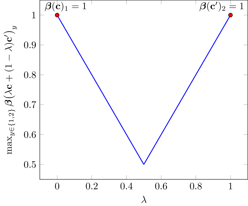
The image displays a 2D line plot showing a V-shaped function. The plot illustrates how a specific mathematical expression, involving a parameter λ and a function β, varies as λ changes from 0 to 1. The function reaches its minimum value at the midpoint (λ=0.5) and its maximum values at the endpoints (λ=0 and λ=1).
### Components/Axes
* **X-Axis:**
* **Label:** `λ` (Greek letter lambda).
* **Scale:** Linear scale from 0 to 1.
* **Tick Marks:** Major ticks at 0, 0.2, 0.4, 0.6, 0.8, and 1.
* **Y-Axis:**
* **Label:** `max_{y∈{1,2}} β(λc + (1-λ)c')_y`. This is a complex mathematical expression indicating the maximum value over y (where y is either 1 or 2) of the function β applied to a convex combination of vectors `c` and `c'`.
* **Scale:** Linear scale from 0.5 to 1.
* **Tick Marks:** Major ticks at 0.5, 0.6, 0.7, 0.8, 0.9, and 1.
* **Data Series:**
* A single blue line connects three key points.
* **Data Points:** Two prominent red circular markers are placed at the endpoints of the line.
* **Annotations:**
* **Top-Left Corner:** Text annotation `β(c)_1 = 1`. This is positioned directly above the red data point at (λ=0, y=1).
* **Top-Right Corner:** Text annotation `β(c')_2 = 1`. This is positioned directly above the red data point at (λ=1, y=1).
### Detailed Analysis
* **Trend Verification:** The blue line exhibits a symmetric V-shape. It slopes downward linearly from the left endpoint to the center, then slopes upward linearly from the center to the right endpoint.
* **Data Points & Values:**
1. **Left Endpoint (λ=0):** The red marker and annotation confirm the value is exactly `y = 1`. The annotation `β(c)_1 = 1` suggests that when λ=0, the convex combination simplifies to vector `c`, and the first component (y=1) of β(c) equals 1.
2. **Minimum Point (λ=0.5):** The blue line reaches its lowest point. The y-value is visually exactly `0.5`. No annotation is present, but the line's vertex aligns perfectly with the 0.5 tick mark.
3. **Right Endpoint (λ=1):** The red marker and annotation confirm the value is exactly `y = 1`. The annotation `β(c')_2 = 1` suggests that when λ=1, the convex combination simplifies to vector `c'`, and the second component (y=2) of β(c') equals 1.
* **Line Segments:**
* From λ=0 to λ=0.5: The line is straight, decreasing from y=1 to y=0.5.
* From λ=0.5 to λ=1: The line is straight, increasing from y=0.5 to y=1.
### Key Observations
1. **Perfect Symmetry:** The plot is perfectly symmetric about the vertical line λ=0.5.
2. **Linear Segments:** The function is piecewise linear, composed of two straight line segments.
3. **Endpoint Maxima:** The maximum value of the function (y=1) occurs at the boundaries of the domain (λ=0 and λ=1).
4. **Midpoint Minimum:** The minimum value of the function (y=0.5) occurs exactly at the midpoint of the domain (λ=0.5).
5. **Annotation Specificity:** The annotations at the endpoints are specific to different components (y=1 for c, y=2 for c'), indicating that the `max` operation selects the larger value between the two components at each λ.
### Interpretation
This plot visualizes a fundamental property of the function `max_{y∈{1,2}} β(λc + (1-λ)c')_y` under the given conditions (`β(c)_1 = 1` and `β(c')_2 = 1`).
* **What the data suggests:** The V-shape demonstrates that the maximum of the two components of β is highest when the input is purely one of the original vectors (`c` or `c'`). As the input becomes a mixture of the two vectors (as λ moves from 0 to 1), the maximum value decreases, reaching its lowest point when the mixture is an equal blend (λ=0.5). This is characteristic of a convex function.
* **Relationship between elements:** The parameter λ controls the interpolation between vectors `c` and `c'`. The y-axis value tracks the "worst-case" or "dominant" output of the function β across its two components for each interpolated vector. The annotations define the boundary conditions that create the symmetric V-shape.
* **Notable pattern:** The linearity of the segments suggests that the function β, or at least its maximum over the two components, behaves linearly with respect to the convex combination parameter λ in this specific example. The exact minimum value of 0.5 at λ=0.5 implies a specific relationship between the components of β(c) and β(c') that leads to this balanced outcome. This could represent a scenario of perfect trade-off or balance between two competing objectives or properties represented by the two components.