## Scatter Plot: college_computer_science ### Overview The image is a scatter plot titled "college_computer_science" showing the relationship between "Target Length" and "Confidence". The plot includes marginal distributions (histograms) for both variables along the axes. The scatter plot shows individual data points and a regression line with a confidence interval shaded around it. ### Components/Axes * **Title:** college_computer_science * **X-axis:** Target Length * Scale: 0 to 100, with tick marks at 0, 50, and 100. * **Y-axis:** Confidence * Scale: 0.2 to 0.8, with tick marks at 0.2, 0.4, 0.6, and 0.8. * **Data Points:** Each point represents a data entry. The points are colored in a light purple. * **Regression Line:** A light purple line shows the linear regression fit to the data. * **Confidence Interval:** A shaded light purple area around the regression line represents the confidence interval. * **Marginal Distribution (X-axis):** A histogram above the scatter plot shows the distribution of "Target Length". * **Marginal Distribution (Y-axis):** A histogram to the right of the scatter plot shows the distribution of "Confidence". ### Detailed Analysis * **Target Length:** The data points are concentrated between 0 and 50, with fewer points beyond 50. * **Confidence:** The confidence values range from approximately 0.2 to 0.8. * **Trend:** The regression line slopes upward, indicating a positive correlation between "Target Length" and "Confidence". * **Data Points:** * At Target Length = 0, Confidence ranges from 0.2 to 0.6. * At Target Length = 50, Confidence ranges from 0.3 to 0.8. * At Target Length = 100, Confidence ranges from 0.5 to 0.8. ### Key Observations * There is a positive correlation between Target Length and Confidence. * The data is more densely populated at lower Target Length values. * The confidence interval widens as Target Length increases, indicating greater uncertainty in the prediction for larger Target Length values. ### Interpretation The scatter plot suggests that as the Target Length increases, the Confidence tends to increase as well. However, the spread of data points indicates that the relationship is not perfectly linear, and there is variability in Confidence for any given Target Length. The widening confidence interval suggests that predictions become less precise as Target Length increases. The concentration of data points at lower Target Length values indicates that the model is more frequently applied to shorter targets.

\n ## Scatter Plot: Confidence vs. Target Length for College Computer Science ### Overview The image presents a scatter plot visualizing the relationship between "Target Length" and "Confidence" for data labeled as "college_computer_science". A regression line with a shaded confidence interval is overlaid on the scatter points. There are also two marginal distributions (histograms) displayed at the top and right sides of the main plot, showing the distributions of Target Length and Confidence respectively. ### Components/Axes * **X-axis:** "Target Length" ranging from approximately 0 to 120. * **Y-axis:** "Confidence" ranging from approximately 0.2 to 0.9. * **Scatter Points:** Numerous purple dots representing individual data points. * **Regression Line:** A purple line representing the trend of the data. The line slopes upwards from left to right. * **Confidence Interval:** A shaded purple area around the regression line, indicating the uncertainty in the estimated trend. * **Top Marginal Distribution:** A histogram showing the distribution of "Target Length". It appears to be skewed to the right, with a concentration of values near 0 and a tail extending towards higher values. * **Right Marginal Distribution:** A histogram showing the distribution of "Confidence". It appears to be roughly symmetrical, with a peak around 0.5-0.6. * **Title:** "college\_computer\_science" positioned at the top-left corner. ### Detailed Analysis The scatter plot shows a positive correlation between "Target Length" and "Confidence". As "Target Length" increases, "Confidence" tends to increase as well. However, the relationship is not perfectly linear, and there is considerable scatter around the regression line. * **Regression Line Trend:** The regression line slopes upwards, indicating a positive correlation. * **Data Point Distribution:** The data points are clustered around the origin (low "Target Length", low "Confidence"). As "Target Length" increases, the points become more dispersed, with some points reaching high "Confidence" values. * **Approximate Data Points (sampled):** * Target Length = 0, Confidence ≈ 0.35 * Target Length = 25, Confidence ≈ 0.55 * Target Length = 50, Confidence ≈ 0.65 * Target Length = 75, Confidence ≈ 0.70 * Target Length = 100, Confidence ≈ 0.75 * **Top Marginal Distribution:** The distribution of "Target Length" is heavily skewed towards lower values. Approximately 70% of the data points have a "Target Length" below 25. * **Right Marginal Distribution:** The distribution of "Confidence" is approximately normal, with a mean around 0.55 and a standard deviation of approximately 0.15. ### Key Observations * The positive correlation between "Target Length" and "Confidence" suggests that longer targets are associated with higher confidence. * The wide confidence interval around the regression line indicates that the relationship is not very strong, and there is considerable uncertainty in the estimated trend. * The skewed distribution of "Target Length" suggests that most targets are relatively short. * The marginal distributions provide additional information about the distributions of the individual variables. ### Interpretation This data likely represents a model's confidence score in predicting or completing tasks of varying lengths within the domain of college-level computer science. The positive correlation suggests that the model performs better (higher confidence) on longer tasks. However, the scatter and the confidence interval indicate that task length is not the sole determinant of confidence; other factors likely play a role. The skewed distribution of target length suggests that the model is primarily evaluated on shorter tasks. The marginal distributions provide context for the main scatter plot. The distribution of target length shows that the model is mostly tested on shorter targets, while the distribution of confidence shows that the model's confidence scores are generally moderate. The data could be used to improve the model by focusing on tasks of varying lengths and identifying factors that contribute to higher confidence scores. It could also be used to assess the model's performance on different types of tasks and identify areas where it needs improvement.

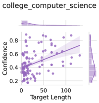
## Scatter Plot with Regression Line: College Computer Science ### Overview The image is a scatter plot titled "college_computer_science" that visualizes the relationship between "Target Length" and "Confidence". It includes a fitted regression line with a shaded confidence interval and marginal histograms showing the distribution of each variable. ### Components/Axes * **Title:** "college_computer_science" (located at the top-left). * **X-Axis:** * **Label:** "Target Length" * **Scale:** Linear, ranging from 0 to approximately 120. Major tick marks are visible at 0, 50, and 100. * **Y-Axis:** * **Label:** "Confidence" * **Scale:** Linear, ranging from 0.2 to 0.8. Major tick marks are visible at 0.2, 0.4, 0.6, and 0.8. * **Data Series:** * **Scatter Points:** Numerous purple circular data points are plotted across the graph. * **Regression Line:** A solid purple line showing the best-fit linear trend. * **Confidence Interval:** A semi-transparent purple shaded area surrounding the regression line, indicating the uncertainty of the fit. * **Marginal Distributions:** * **Top Histogram:** A horizontal histogram positioned above the main plot, showing the distribution of the "Target Length" (x-axis) data. It is heavily right-skewed, with the highest frequency near 0. * **Right Histogram:** A vertical histogram positioned to the right of the main plot, showing the distribution of the "Confidence" (y-axis) data. It appears roughly unimodal, centered around 0.4-0.5. ### Detailed Analysis * **Data Point Distribution:** The scatter points are densely clustered in the lower-left quadrant of the plot, specifically where "Target Length" is between 0-40 and "Confidence" is between 0.2-0.6. The density of points decreases as both values increase. * **Trend Verification:** The purple regression line has a clear positive slope, indicating a direct correlation. It originates near the coordinate (0, 0.4) and extends to approximately (120, 0.7). * **Key Data Points (Approximate):** * Lowest Confidence Point: ~ (5, 0.2) * Highest Confidence Point: ~ (100, 0.8) * Highest Target Length Point: ~ (115, 0.65) * **Marginal Histogram Details:** * The "Target Length" histogram shows the vast majority of observations have a length less than 50, with a very long tail extending to 120. * The "Confidence" histogram shows most values fall between 0.3 and 0.6. ### Key Observations 1. **Positive Correlation:** There is a clear, positive linear relationship between Target Length and Confidence. As the target length increases, the confidence score tends to increase. 2. **Heteroscedasticity:** The spread (variance) of the Confidence values appears to increase slightly as Target Length increases. The data is more tightly clustered at low Target Lengths and becomes more dispersed at higher values. 3. **Data Skew:** Both variables are not normally distributed. Target Length is strongly right-skewed, and Confidence is somewhat left-skewed (more mass on the lower end). 4. **Outliers:** A few data points exist with high Confidence (>0.7) at moderate Target Lengths (~50-80), which sit above the main cluster and the confidence interval band. ### Interpretation The data suggests that in the context of "college computer science," tasks or items with a longer "Target Length" (which could refer to answer length, code length, or document length) are associated with higher "Confidence" (potentially model confidence, grader confidence, or student confidence). This could imply that more substantial or detailed responses are perceived as more reliable or are generated with higher certainty by an automated system. The strong skew in Target Length indicates that most tasks are short, but the few long tasks are associated with higher confidence. The increasing variance (heteroscedasticity) suggests that while confidence generally rises with length, predictions for longer targets become less precise. The marginal histograms provide crucial context, showing that the observed positive trend is driven by a minority of data points with high Target Length, as most data is concentrated at the low end. This is a classic example where the summary statistic (the regression line) tells an important story, but the underlying data distribution reveals the full, nuanced picture.

## Scatter Plot: college_computer_science ### Overview The image is a scatter plot titled "college_computer_science" with a linear regression trend line and shaded confidence interval. It includes marginal histograms on the top and right. The plot visualizes the relationship between "Target Length" (x-axis) and "Confidence" (y-axis), with data points represented as purple dots. ### Components/Axes - **Title**: "college_computer_science" (top-center). - **X-axis**: "Target Length" (0 to 100, labeled at bottom). - **Y-axis**: "Confidence" (0.2 to 0.8, labeled at left). - **Trend Line**: A purple line with a shaded confidence interval (purple gradient). - **Marginal Histograms**: - Top histogram: Distribution of "Target Length" (purple bars). - Right histogram: Distribution of "Confidence" (purple bars). ### Detailed Analysis - **Data Points**: - Purple dots scattered across the plot, with higher density near the trend line. - Confidence values range from ~0.2 to ~0.8, with most points clustered between 0.4 and 0.6. - **Trend Line**: - Slope: Positive (increasing Confidence with Target Length). - Confidence Interval: Shaded area narrows as Target Length increases, indicating reduced variability at higher lengths. - **Histograms**: - **Target Length**: Skewed right, with most values between 0 and 50. - **Confidence**: Peaks near 0.5–0.6, with a gradual decline toward 0.2 and 0.8. ### Key Observations 1. **Positive Correlation**: Confidence increases with Target Length (e.g., at Target Length = 50, Confidence ≈ 0.5; at Target Length = 100, Confidence ≈ 0.7). 2. **Confidence Interval Narrowing**: The shaded area becomes tighter at higher Target Lengths, suggesting more consistent relationships. 3. **Distribution Patterns**: - Target Length is more variable (wide spread in the top histogram). - Confidence is concentrated around the trend line (narrower distribution in the right histogram). ### Interpretation The data suggests a **positive relationship** between Target Length and Confidence in college computer science contexts. Longer Target Lengths are associated with higher Confidence, and the narrowing confidence interval at higher lengths implies greater reliability in this trend. The histograms reveal that while Target Length varies widely, Confidence is more clustered, particularly around the trend line. This could indicate that longer projects or courses in computer science may correlate with increased student confidence, though variability persists, especially for shorter lengths. The marginal histograms highlight the need to consider both central tendency and distribution when interpreting the relationship.