## Line Chart: C^(q)(Γ) vs. Γ for different values of x ### Overview The image presents two line charts side-by-side, both plotting C^(q)(Γ) against Γ. The charts display the relationship between these variables for different constant values of 'x', ranging from 0.1 to 2.0. The left chart shows the behavior of the function from Γ = 0 to 8, while the right chart appears to focus on a specific region where the function exhibits more rapid changes. ### Components/Axes * **X-axis (Horizontal):** Γ (Gamma), ranging from 0 to 8 in both charts. * **Y-axis (Vertical):** C^(q)(Γ), ranging from -1 to 1 in both charts. * **Legend (Top-Right of each chart):** * x = 0.1 (Solid Line) * x = 0.2 (Dashed Line) * x = 0.5 (Dotted Line) * x = 1.0 (Dash-Dot Line) * x = 2.0 (Long Dash Line) ### Detailed Analysis **Left Chart:** * **x = 0.1 (Solid Line):** Starts at approximately 0.95 at Γ = 0 and decreases rapidly, approaching 0 at Γ = 4 and remaining close to 0 for Γ > 4. * **x = 0.2 (Dashed Line):** Starts at approximately 0.8 at Γ = 0 and decreases, approaching 0 at Γ = 4 and remaining close to 0 for Γ > 4. * **x = 0.5 (Dotted Line):** Starts at approximately 0.3 at Γ = 0 and decreases, becoming negative around Γ = 1, reaching approximately -0.25 at Γ = 2, and then slowly approaching 0 for Γ > 4. * **x = 1.0 (Dash-Dot Line):** Starts at approximately -0.3 at Γ = 0 and increases, approaching 0 at Γ = 4 and remaining close to 0 for Γ > 4. * **x = 2.0 (Long Dash Line):** Starts at approximately -1 at Γ = 0 and increases, approaching 0 at Γ = 4 and remaining close to 0 for Γ > 4. **Right Chart:** * **x = 0.1 (Solid Line):** Starts at approximately 1 and decreases rapidly, approaching 0.1 at Γ = 4 and remaining close to 0.1 for Γ > 4. * **x = 0.2 (Dashed Line):** Starts at approximately 1 and decreases rapidly, approaching 0 at Γ = 4 and remaining close to 0 for Γ > 4. * **x = 0.5 (Dotted Line):** Starts at approximately -0.9 at Γ = 0 and increases rapidly, approaching 0 at Γ = 4 and remaining close to 0 for Γ > 4. * **x = 1.0 (Dash-Dot Line):** Starts at approximately -0.9 at Γ = 0 and increases rapidly, approaching 0 at Γ = 4 and remaining close to 0 for Γ > 4. * **x = 2.0 (Long Dash Line):** Starts at approximately -0.9 at Γ = 0 and increases rapidly, approaching 0 at Γ = 4 and remaining close to 0 for Γ > 4. ### Key Observations * For smaller values of 'x' (0.1 and 0.2), C^(q)(Γ) starts positive and decreases towards zero as Γ increases. * For larger values of 'x' (0.5, 1.0, and 2.0), C^(q)(Γ) starts negative and increases towards zero as Γ increases. * The right chart shows a zoomed-in view of the initial behavior of the curves, highlighting the rapid changes near Γ = 0. * All curves tend to converge towards zero as Γ increases, suggesting a limiting behavior of the function. ### Interpretation The charts illustrate how the function C^(q)(Γ) behaves as Γ varies, for different fixed values of 'x'. The data suggests that 'x' influences the initial value and the direction of change of C^(q)(Γ). Smaller 'x' values lead to positive initial values and a decreasing trend, while larger 'x' values lead to negative initial values and an increasing trend. The convergence of all curves towards zero as Γ increases indicates that the influence of 'x' diminishes as Γ becomes large. The right chart emphasizes the sensitivity of C^(q)(Γ) to changes in Γ, especially when Γ is small. The relationship between 'x' and C^(q)(Γ) appears to be inversely proportional at Γ = 0.

\n ## Chart: Correlation Function vs. Gamma ### Overview The image presents a chart displaying the correlation function, C^(ω)(Γ), as a function of Gamma (Γ) for different values of 'x'. The chart is split into two panels, likely representing different conditions or scales. Each panel shows five curves, each corresponding to a specific 'x' value. ### Components/Axes * **X-axis:** Gamma (Γ), ranging from approximately 0 to 8. * **Y-axis:** Correlation Function C^(ω)(Γ), ranging from approximately -1 to 0.75. * **Legend:** Located in the top-right corner of each panel, listing the 'x' values and their corresponding line styles: * x = 0.1 (solid line) * x = 0.2 (dashed line) * x = 0.5 (dotted line) * x = 1.0 (dash-dot line) * x = 2.0 (long dash-dot line) ### Detailed Analysis The chart consists of two identical panels, side-by-side. We will analyze one panel and assume the other exhibits the same trends. **Left Panel:** * **x = 0.1 (solid line):** Starts at approximately 0.6, rapidly decreases to around 0.1 at Γ ≈ 1, and then plateaus around 0.05 for Γ > 2. * **x = 0.2 (dashed line):** Starts at approximately 0.3, decreases more gradually than x=0.1, reaching around 0 at Γ ≈ 3, and remains near 0 for larger Γ. * **x = 0.5 (dotted line):** Starts at approximately 0.1, decreases to a minimum of around -0.25 at Γ ≈ 2, and then slowly increases, approaching 0 for Γ > 6. * **x = 1.0 (dash-dot line):** Starts at approximately -0.1, decreases to a minimum of around -0.5 at Γ ≈ 2, and then slowly increases, approaching 0 for Γ > 6. * **x = 2.0 (long dash-dot line):** Starts at approximately -0.3, rapidly decreases to a minimum of around -1 at Γ ≈ 1, and then slowly increases, approaching 0 for Γ > 6. **Right Panel:** The trends in the right panel are identical to those in the left panel. ### Key Observations * The curves exhibit significant changes in behavior around Γ ≈ 1-2. * Higher values of 'x' generally lead to more negative correlation function values, especially at lower Γ. * For all 'x' values, the correlation function tends to approach 0 as Γ increases. * The solid line (x=0.1) remains positive throughout the range of Γ, while the other lines become negative. ### Interpretation This chart likely represents the correlation function in a physical system, possibly a plasma or a condensed matter system. The parameter 'x' could represent a control parameter such as density or interaction strength. The Gamma (Γ) parameter could represent a frequency or a damping rate. The fact that the correlation function becomes negative for higher 'x' values suggests a transition to a state with anti-correlation. The rapid changes around Γ ≈ 1-2 could indicate a resonance or instability in the system. The approach to zero correlation at high Γ suggests that the system becomes more disordered or that correlations are screened out at higher frequencies or damping rates. The two panels being identical suggests that the observed behavior is consistent and not dependent on specific experimental conditions. The chart provides insights into the collective behavior of the system and how it changes with the control parameter 'x'. The negative correlation for higher x values is a particularly interesting feature, potentially indicating a change in the fundamental nature of the interactions within the system.

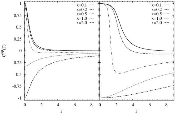
## Scientific Plot: Dual-Panel Function Analysis ### Overview The image displays a two-panel scientific plot, likely from a physics or engineering context, showing the behavior of a function denoted as `C^(0)(Γ)` against a variable `Γ`. Each panel contains multiple curves corresponding to different values of a parameter `x`. The left panel shows curves that generally decay or rise towards zero, while the right panel shows more complex, non-monotonic behavior with curves that dip and then recover. ### Components/Axes * **Layout:** Two rectangular plot panels arranged side-by-side, sharing a common x-axis label. * **Left Panel:** * **Y-axis Label:** `C^(0)(Γ)` (vertical text, left side). * **Y-axis Scale:** Linear, ranging from -1.0 to 1.0, with major ticks at intervals of 0.25 (-1, -0.75, -0.5, -0.25, 0, 0.25, 0.5, 0.75, 1). * **X-axis Label:** `Γ` (centered below the axis). * **X-axis Scale:** Linear, ranging from 0 to 8, with major ticks at 0, 2, 4, 6, 8. * **Right Panel:** * **Y-axis Label:** Not explicitly labeled. It shares the same scale and range as the left panel. * **X-axis Label:** `Γ` (centered below the axis). * **X-axis Scale:** Linear, ranging from 0 to 8, with major ticks at 0, 2, 4, 6, 8. * **Legend:** Located in the top-right corner of each panel. It defines five curves by the parameter `x` and their corresponding line styles: * `x=0.1` - Solid line * `x=0.2` - Dashed line (long dashes) * `x=0.5` - Dotted line (short dots) * `x=1.0` - Solid line (thinner weight than x=0.1) * `x=2.0` - Dash-dot line ### Detailed Analysis **Left Panel Analysis:** * **Trend:** All curves originate at `Γ=0` and approach the horizontal axis (`C^(0)(Γ) = 0`) as `Γ` increases, suggesting a decay or relaxation process. * **Data Series & Approximate Points:** * **x=0.1 (Solid):** Starts at `C^(0)(0) ≈ 1.0`. Decays rapidly, crossing `C^(0) ≈ 0.25` near `Γ ≈ 0.5`, and approaches zero asymptotically. * **x=0.2 (Dashed):** Starts at `C^(0)(0) ≈ 1.0`. Decays slower than x=0.1, crossing `C^(0) ≈ 0.25` near `Γ ≈ 1.0`. * **x=0.5 (Dotted):** Starts at `C^(0)(0) ≈ 1.0`. Decays more slowly, crossing `C^(0) ≈ 0.25` near `Γ ≈ 2.0`. * **x=1.0 (Thin Solid):** Starts at `C^(0)(0) ≈ -0.3`. Rises monotonically, approaching zero from below. * **x=2.0 (Dash-Dot):** Starts at `C^(0)(0) ≈ -1.0`. Rises monotonically, approaching zero from below, but remains more negative than the x=1.0 curve for all `Γ`. **Right Panel Analysis:** * **Trend:** Curves exhibit non-monotonic behavior. They start at extreme values (`1` or `-1`), undergo a significant dip or rise, and then trend back towards zero or a negative asymptote. * **Data Series & Approximate Points:** * **x=0.1 (Solid):** Starts at `C^(0)(0) ≈ 1.0`. Remains near 1 until `Γ ≈ 1`, then decays smoothly, crossing `C^(0) ≈ 0.5` near `Γ ≈ 2.5`, and approaches zero. * **x=0.2 (Dashed):** Starts at `C^(0)(0) ≈ 1.0`. Begins decaying earlier than x=0.1, crossing `C^(0) ≈ 0.5` near `Γ ≈ 1.5`, and approaches zero. * **x=0.5 (Dotted):** Starts at `C^(0)(0) ≈ 1.0`. Drops sharply, reaching a minimum of `C^(0) ≈ -0.5` near `Γ ≈ 2.5`, then rises, crossing zero near `Γ ≈ 5.5` and approaching a small positive value. * **x=1.0 (Thin Solid):** Starts at `C^(0)(0) ≈ -1.0`. Rises steadily, crossing `C^(0) ≈ -0.5` near `Γ ≈ 3.0` and `C^(0) ≈ 0` near `Γ ≈ 7.0`. * **x=2.0 (Dash-Dot):** Starts at `C^(0)(0) ≈ -1.0`. Rises more slowly than x=1.0, crossing `C^(0) ≈ -0.75` near `Γ ≈ 4.0`. ### Key Observations 1. **Parameter `x` Controls Dynamics:** The parameter `x` dramatically alters the functional form. Low `x` (0.1, 0.2) leads to simple decay from a positive initial condition. Intermediate `x` (0.5) causes an undershoot below zero before recovery. High `x` (1.0, 2.0) leads to growth from a negative initial condition. 2. **Initial Condition Split:** There is a clear bifurcation at `x=1.0`. For `x < 1`, `C^(0)(0) = 1`. For `x ≥ 1`, `C^(0)(0) = -1` (or near -1 for x=1.0). 3. **Asymptotic Behavior:** In the left panel, all curves converge to 0. In the right panel, curves for `x ≤ 0.2` converge to 0, while curves for `x ≥ 0.5` appear to converge to different negative or near-zero values. 4. **Crossing Points:** The `x=0.5` curve in the right panel is notable for crossing from positive to negative and back to positive, indicating a complex underlying process. ### Interpretation This plot likely illustrates the solution to a differential equation or a response function where `x` is a critical control parameter (e.g., coupling strength, damping coefficient, or a ratio of timescales). The left panel might represent a standard or baseline response, showing how perturbations (`C^(0)`) decay over time (`Γ`). The right panel could represent a different regime or a related but distinct quantity, where the system exhibits resonant or oscillatory-like behavior (the dip and recovery) for intermediate `x`. The sharp change in initial condition at `x=1.0` suggests a phase transition or a bifurcation point in the system's dynamics. The non-monotonic response for `x=0.5` is particularly significant, as it indicates the system can temporarily overshoot its equilibrium state. The divergence in asymptotic behavior in the right panel implies that the parameter `x` not only affects the transient response but also the final steady state of the system. This type of analysis is fundamental in fields like control theory, statistical mechanics, or signal processing to understand system stability and parameter sensitivity.

## Line Graph: Behavior of C^(q)(Γ) Across Γ Values for Different x Parameters ### Overview The image contains two mirrored line graphs side-by-side, depicting the relationship between Γ (horizontal axis) and C^(q)(Γ) (vertical axis) for five distinct x values (0.1, 0.2, 0.5, 1.0, 2.0). The left graph spans Γ = 0 to 8, while the right graph spans Γ = -8 to 0. Each x value is represented by a unique line style (solid, dashed, dotted, etc.), with curves showing distinct trends in C^(q)(Γ) as Γ varies. --- ### Components/Axes - **Left Graph (Γ ≥ 0):** - **X-axis (Γ):** Labeled Γ, ranging from 0 to 8 in increments of 2. - **Y-axis (C^(q)(Γ)):** Labeled C^(q)(Γ), ranging from -1 to 1 in increments of 0.25. - **Legend:** Positioned at the top-left, associating line styles with x values: - x=0.1: Solid line - x=0.2: Dashed line - x=0.5: Dotted line - x=1.0: Dash-dot line - x=2.0: Double-dash line - **Right Graph (Γ ≤ 0):** - **X-axis (Γ):** Labeled Γ, ranging from -8 to 0 in increments of 2. - **Y-axis (C^(q)(Γ)):** Same scale as the left graph (-1 to 1). - **Legend:** Positioned at the top-right, mirroring the left graph's legend. --- ### Detailed Analysis #### Left Graph (Γ ≥ 0) 1. **x=0.1 (Solid Line):** - Starts near 1 at Γ=0, sharply declines to ~0.25 by Γ=2, then plateaus. - **Key Trend:** Rapid initial decay followed by stabilization. 2. **x=0.2 (Dashed Line):** - Begins at ~0.75, declines gradually to ~0.1 by Γ=4, then flattens. - **Key Trend:** Slower decay than x=0.1, with a longer plateau. 3. **x=0.5 (Dotted Line):** - Starts at ~0.5, declines to ~-0.25 by Γ=6, then rises slightly. - **Key Trend:** Crosses into negative territory before stabilizing. 4. **x=1.0 (Dash-Dot Line):** - Begins at ~0.25, declines to ~-0.75 by Γ=4, then sharply rises to ~-0.25 by Γ=8. - **Key Trend:** Strong negative dip followed by recovery. 5. **x=2.0 (Double-Dash Line):** - Starts at ~-0.5, declines to ~-0.9 by Γ=2, then rises to ~-0.5 by Γ=8. - **Key Trend:** Initial sharp drop followed by partial recovery. #### Right Graph (Γ ≤ 0) 1. **x=0.1 (Solid Line):** - Starts near -1 at Γ=-8, rises to ~-0.25 by Γ=-2, then plateaus. - **Key Trend:** Gradual ascent from a deep negative value. 2. **x=0.2 (Dashed Line):** - Begins at ~-0.75, rises to ~-0.1 by Γ=-4, then flattens. - **Key Trend:** Moderate recovery from negative values. 3. **x=0.5 (Dotted Line):** - Starts at ~-0.5, rises to ~0.25 by Γ=-6, then dips slightly. - **Key Trend:** Crosses into positive territory before stabilizing. 4. **x=1.0 (Dash-Dot Line):** - Begins at ~0.25, rises to ~0.75 by Γ=-4, then sharply drops to ~0.25 by Γ=0. - **Key Trend:** Sharp positive peak followed by decline. 5. **x=2.0 (Double-Dash Line):** - Starts at ~-0.5, rises to ~0.5 by Γ=-2, then drops to ~-0.5 by Γ=0. - **Key Trend:** Symmetric V-shaped curve. --- ### Key Observations 1. **Symmetry:** The right graph mirrors the left graph's behavior but with inverted Γ values (e.g., x=0.1's solid line on the left peaks at Γ=0, while on the right it starts at Γ=-8). 2. **x-Dependent Behavior:** - Lower x values (0.1–0.5) exhibit smoother transitions. - Higher x values (1.0–2.0) show sharper inflection points and greater amplitude swings. 3. **Asymptotic Behavior:** All curves approach horizontal asymptotes as |Γ| increases, suggesting saturation effects. 4. **Negative Γ Dominance:** For x ≥ 1.0, the right graph (Γ ≤ 0) shows more pronounced oscillations compared to the left graph. --- ### Interpretation The data suggests that C^(q)(Γ) is highly sensitive to both Γ and x parameters. The mirrored symmetry implies a potential relationship where positive and negative Γ values exhibit complementary behaviors for a given x. The sharp transitions at intermediate Γ values (e.g., x=1.0 and x=2.0) may indicate threshold effects or phase changes in the system being modeled. The flattening of curves at extreme Γ values suggests diminishing returns or saturation limits. This could represent phenomena such as signal attenuation, material stress responses, or thermodynamic equilibria, depending on the context of the original study.