## Chart/Diagram Type: Probability vs. V_inj Plots
### Overview
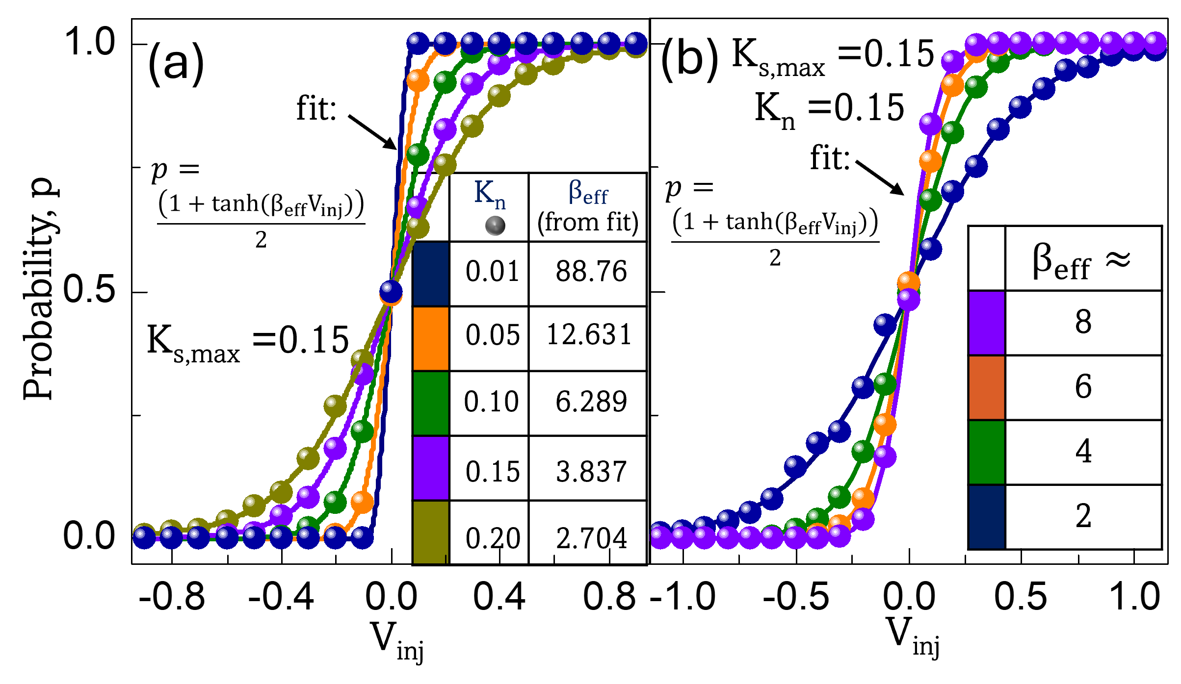
The image presents two plots, (a) and (b), each showing the probability 'p' as a function of V_inj (injection voltage). Both plots display sigmoidal curves, with 'p' increasing as V_inj increases. The plots explore the impact of different parameters on this relationship. Plot (a) shows the effect of varying K_n while keeping K_s,max constant, and plot (b) shows the effect of varying β_eff. Each plot includes a table summarizing the parameter values used for each curve.
### Components/Axes
* **Plot Titles:** (a) and (b)
* **Y-axis Title:** Probability, p
* Scale: 0.0 to 1.0, with tick marks at 0.0, 0.5, and 1.0
* **X-axis Title:** V_inj
* Plot (a) Scale: -0.8 to 0.8, with tick marks at -0.8, -0.4, 0.0, 0.4, and 0.8
* Plot (b) Scale: -1.0 to 1.0, with tick marks at -1.0, -0.5, 0.0, 0.5, and 1.0
* **Equations:** Both plots include the equation: p = (1 + tanh(β_eff \* V_inj)) / 2
* **Plot (a) Table:**
| K_n | β_eff (from fit) |
|------|-------------------|
| 0.01 | 88.76 |
| 0.05 | 12.631 |
| 0.10 | 6.289 |
| 0.15 | 3.837 |
| 0.20 | 2.704 |
* **Plot (b) Table:**
| β_eff ≈ |
|---------|
| 8 (Purple) |
| 6 (Orange) |
| 4 (Green) |
| 2 (Dark Blue) |
* **Constants:**
* Plot (a): K_s,max = 0.15
* Plot (b): K_s,max = 0.15, K_n = 0.15
### Detailed Analysis or ### Content Details
**Plot (a):**
* **Dark Blue Line (K_n = 0.01):** This line has the steepest slope and reaches a probability of 1.0 at approximately V_inj = 0.2. It starts at a probability of approximately 0.0 for V_inj < -0.4.
* **Orange Line (K_n = 0.05):** This line has a shallower slope than the dark blue line. It reaches a probability of 1.0 at approximately V_inj = 0.4.
* **Green Line (K_n = 0.10):** This line has a shallower slope than the orange line. It reaches a probability of 1.0 at approximately V_inj = 0.6.
* **Purple Line (K_n = 0.15):** This line has a shallower slope than the green line. It reaches a probability of 1.0 at approximately V_inj = 0.8.
* **Olive Line (K_n = 0.20):** This line has the shallowest slope. It reaches a probability of 1.0 at approximately V_inj = 1.0.
**Plot (b):**
* **Dark Blue Line (β_eff ≈ 2):** This line has the shallowest slope. It reaches a probability of 1.0 at approximately V_inj = 1.0.
* **Green Line (β_eff ≈ 4):** This line has a steeper slope than the dark blue line. It reaches a probability of 1.0 at approximately V_inj = 0.6.
* **Orange Line (β_eff ≈ 6):** This line has a steeper slope than the green line. It reaches a probability of 1.0 at approximately V_inj = 0.4.
* **Purple Line (β_eff ≈ 8):** This line has the steepest slope. It reaches a probability of 1.0 at approximately V_inj = 0.2.
### Key Observations
* In plot (a), as K_n increases, the slope of the curve decreases, indicating a less sensitive response of probability to changes in V_inj.
* In plot (b), as β_eff increases, the slope of the curve increases, indicating a more sensitive response of probability to changes in V_inj.
* The equation p = (1 + tanh(β_eff \* V_inj)) / 2 is used to fit the data in both plots.
### Interpretation
The plots demonstrate the relationship between injection voltage (V_inj) and probability (p), influenced by parameters K_n and β_eff. Plot (a) shows that increasing K_n, while keeping K_s,max constant, reduces the sensitivity of the probability to changes in V_inj. This suggests that a higher K_n value requires a larger change in V_inj to achieve the same change in probability. Plot (b) shows that increasing β_eff increases the sensitivity of the probability to changes in V_inj. This indicates that a higher β_eff value results in a larger change in probability for the same change in V_inj. The equation used to fit the data suggests a sigmoidal relationship between V_inj and probability, which is consistent with the observed curves. The plots provide insights into how different parameters can modulate the response of a system to an input voltage.