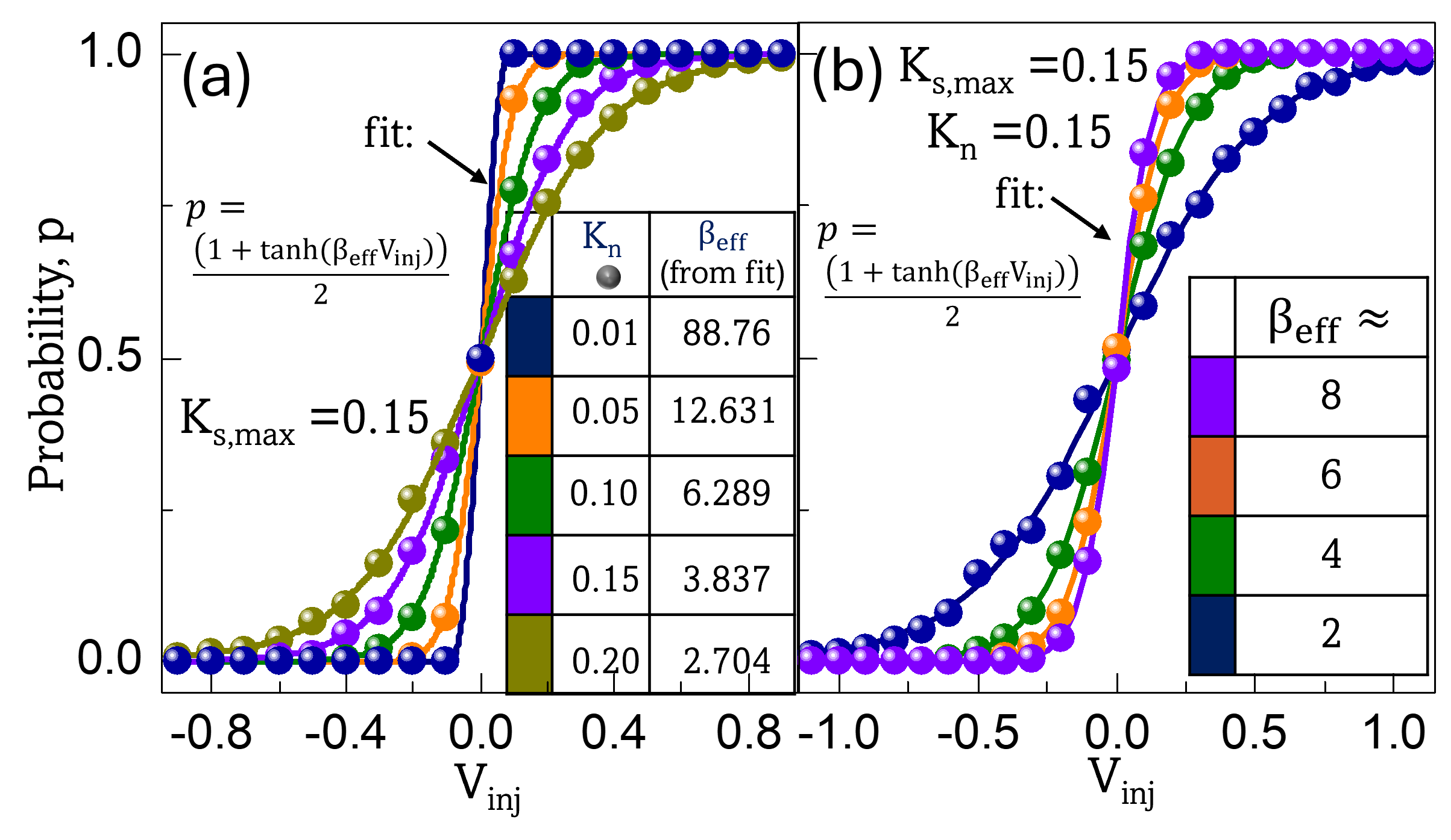
## [Chart Type]: Probability vs. Injection Voltage (Two Panels: (a) and (b)) ### Overview The image contains two side-by-side plots (labeled (a) and (b)) showing the probability \( p \) of a process (e.g., injection success) as a function of injection voltage \( V_{\text{inj}} \). Both plots use a sigmoidal (tanh-based) fit: \( p = \frac{1 + \tanh(\beta_{\text{eff}} V_{\text{inj}})}{2} \), with different parameter sets ( \( K_n \) in (a), \( \beta_{\text{eff}} \) in (b)). ### Components/Axes #### Panel (a) (Left): - **Title/Label**: (a) with \( K_{s,\text{max}} = 0.15 \). - **Axes**: - Y-axis: Probability, \( p \) (range: \( 0.0 \) to \( 1.0 \)). - X-axis: Injection voltage, \( V_{\text{inj}} \) (range: \( -0.8 \) to \( 0.8 \)). - **Equation**: \( p = \frac{1 + \tanh(\beta_{\text{eff}} V_{\text{inj}})}{2} \) (labeled "fit:"). - **Legend/Table**: A table maps colors to \( K_n \) and \( \beta_{\text{eff}} \): | Color | \( K_n \) | \( \beta_{\text{eff}} \) | |-------|----------|------------------------| | Dark blue | 0.01 | 88.76 | | Orange | 0.05 | 12.631 | | Green | 0.10 | 6.289 | | Purple | 0.15 | 3.837 | | Olive | 0.20 | 2.704 | #### Panel (b) (Right): - **Title/Label**: (b) with \( K_{s,\text{max}} = 0.15 \), \( K_n = 0.15 \). - **Axes**: - Y-axis: Probability, \( p \) (range: \( 0.0 \) to \( 1.0 \)). - X-axis: Injection voltage, \( V_{\text{inj}} \) (range: \( -1.0 \) to \( 1.0 \)). - **Equation**: Same as (a): \( p = \frac{1 + \tanh(\beta_{\text{eff}} V_{\text{inj}})}{2} \) (labeled "fit:"). - **Legend/Table**: A table maps colors to \( \beta_{\text{eff}} \approx \): | Color | \( \beta_{\text{eff}} \approx \) | |-------|-------------------------------| | Purple | 8 | | Orange | 6 | | Green | 4 | | Dark blue | 2 | ### Detailed Analysis (Data Points & Trends) #### Panel (a) (Varying \( K_n \), \( K_{s,\text{max}} = 0.15 \)): - **Dark blue (\( K_n = 0.01 \), \( \beta_{\text{eff}} = 88.76 \))**: - \( V_{\text{inj}} \approx -0.8 \): \( p \approx 0.0 \) - \( V_{\text{inj}} \approx -0.4 \): \( p \approx 0.0 \) - \( V_{\text{inj}} \approx 0.0 \): \( p \approx 0.5 \) (crossing point) - \( V_{\text{inj}} \approx 0.4 \): \( p \approx 1.0 \) - \( V_{\text{inj}} \approx 0.8 \): \( p \approx 1.0 \) - **Trend**: Steepest curve (highest \( \beta_{\text{eff}} \)), fastest transition from \( p \approx 0 \) to \( p \approx 1 \). - **Orange (\( K_n = 0.05 \), \( \beta_{\text{eff}} = 12.631 \))**: - \( V_{\text{inj}} \approx -0.8 \): \( p \approx 0.0 \) - \( V_{\text{inj}} \approx -0.4 \): \( p \approx 0.0 \) - \( V_{\text{inj}} \approx 0.0 \): \( p \approx 0.5 \) - \( V_{\text{inj}} \approx 0.4 \): \( p \approx 1.0 \) - \( V_{\text{inj}} \approx 0.8 \): \( p \approx 1.0 \) - **Trend**: Less steep than dark blue, more than green. - **Green (\( K_n = 0.10 \), \( \beta_{\text{eff}} = 6.289 \))**: - \( V_{\text{inj}} \approx -0.8 \): \( p \approx 0.0 \) - \( V_{\text{inj}} \approx -0.4 \): \( p \approx 0.0 \) - \( V_{\text{inj}} \approx 0.0 \): \( p \approx 0.5 \) - \( V_{\text{inj}} \approx 0.4 \): \( p \approx 1.0 \) - \( V_{\text{inj}} \approx 0.8 \): \( p \approx 1.0 \) - **Trend**: Less steep than orange, more than purple. - **Purple (\( K_n = 0.15 \), \( \beta_{\text{eff}} = 3.837 \))**: - \( V_{\text{inj}} \approx -0.8 \): \( p \approx 0.0 \) - \( V_{\text{inj}} \approx -0.4 \): \( p \approx 0.0 \) - \( V_{\text{inj}} \approx 0.0 \): \( p \approx 0.5 \) - \( V_{\text{inj}} \approx 0.4 \): \( p \approx 1.0 \) - \( V_{\text{inj}} \approx 0.8 \): \( p \approx 1.0 \) - **Trend**: Less steep than green, more than olive. - **Olive (\( K_n = 0.20 \), \( \beta_{\text{eff}} = 2.704 \))**: - \( V_{\text{inj}} \approx -0.8 \): \( p \approx 0.0 \) - \( V_{\text{inj}} \approx -0.4 \): \( p \approx 0.0 \) - \( V_{\text{inj}} \approx 0.0 \): \( p \approx 0.5 \) - \( V_{\text{inj}} \approx 0.4 \): \( p \approx 1.0 \) - \( V_{\text{inj}} \approx 0.8 \): \( p \approx 1.0 \) - **Trend**: Least steep curve (lowest \( \beta_{\text{eff}} \)), slowest transition. #### Panel (b) (Varying \( \beta_{\text{eff}} \), \( K_{s,\text{max}} = 0.15 \), \( K_n = 0.15 \)): - **Purple (\( \beta_{\text{eff}} \approx 8 \))**: - \( V_{\text{inj}} \approx -1.0 \): \( p \approx 0.0 \) - \( V_{\text{inj}} \approx -0.5 \): \( p \approx 0.0 \) - \( V_{\text{inj}} \approx 0.0 \): \( p \approx 0.5 \) - \( V_{\text{inj}} \approx 0.5 \): \( p \approx 1.0 \) - \( V_{\text{inj}} \approx 1.0 \): \( p \approx 1.0 \) - **Trend**: Steepest curve (highest \( \beta_{\text{eff}} \)), fastest transition. - **Orange (\( \beta_{\text{eff}} \approx 6 \))**: - \( V_{\text{inj}} \approx -1.0 \): \( p \approx 0.0 \) - \( V_{\text{inj}} \approx -0.5 \): \( p \approx 0.0 \) - \( V_{\text{inj}} \approx 0.0 \): \( p \approx 0.5 \) - \( V_{\text{inj}} \approx 0.5 \): \( p \approx 1.0 \) - \( V_{\text{inj}} \approx 1.0 \): \( p \approx 1.0 \) - **Trend**: Less steep than purple, more than green. - **Green (\( \beta_{\text{eff}} \approx 4 \))**: - \( V_{\text{inj}} \approx -1.0 \): \( p \approx 0.0 \) - \( V_{\text{inj}} \approx -0.5 \): \( p \approx 0.0 \) - \( V_{\text{inj}} \approx 0.0 \): \( p \approx 0.5 \) - \( V_{\text{inj}} \approx 0.5 \): \( p \approx 1.0 \) - \( V_{\text{inj}} \approx 1.0 \): \( p \approx 1.0 \) - **Trend**: Less steep than orange, more than dark blue. - **Dark blue (\( \beta_{\text{eff}} \approx 2 \))**: - \( V_{\text{inj}} \approx -1.0 \): \( p \approx 0.0 \) - \( V_{\text{inj}} \approx -0.5 \): \( p \approx 0.0 \) - \( V_{\text{inj}} \approx 0.0 \): \( p \approx 0.5 \) - \( V_{\text{inj}} \approx 0.5 \): \( p \approx 1.0 \) - \( V_{\text{inj}} \approx 1.0 \): \( p \approx 1.0 \) - **Trend**: Least steep curve (lowest \( \beta_{\text{eff}} \)), slowest transition. ### Key Observations 1. **Sigmoidal Transition**: All curves follow \( p = \frac{1 + \tanh(\beta_{\text{eff}} V_{\text{inj}})}{2} \), showing a threshold-like transition from \( p \approx 0 \) to \( p \approx 1 \) around \( V_{\text{inj}} = 0 \). 2. **Parameter Dependence**: - In (a), lower \( K_n \) (higher \( \beta_{\text{eff}} \)) increases curve steepness (faster transition). - In (b), higher \( \beta_{\text{eff}} \) increases curve steepness (faster transition). 3. **Crossing Point**: All curves cross at \( V_{\text{inj}} = 0 \), \( p = 0.5 \), consistent with \( \tanh(0) = 0 \). ### Interpretation - The plots model a threshold-like process (e.g., injection success) where probability depends on \( V_{\text{inj}} \) and parameters \( K_n \) (or \( \beta_{\text{eff}} \)). - The tanh function captures a sigmoidal transition, typical of systems with a sharp threshold (e.g., switching from low to high probability as \( V_{\text{inj}} \) crosses 0). - Lower \( K_n \) (or higher \( \beta_{\text{eff}} \)) makes the process more sensitive to \( V_{\text{inj}} \) near the threshold (steeper transition), implying smaller \( K_n \) (or larger \( \beta_{\text{eff}} \)) enhances the "sharpness" of the threshold behavior. - The consistent crossing point (\( V_{\text{inj}} = 0 \), \( p = 0.5 \)) suggests the threshold is fixed at \( V_{\text{inj}} = 0 \), but the transition rate (steepness) depends on \( K_n \) or \( \beta_{\text{eff}} \). This analysis provides a complete description of the image’s content, trends, and implications, enabling reconstruction of the data and relationships without the original image.