## Chart/Diagram Type: Probability vs. Injected Voltage with Fit Parameters
### Overview
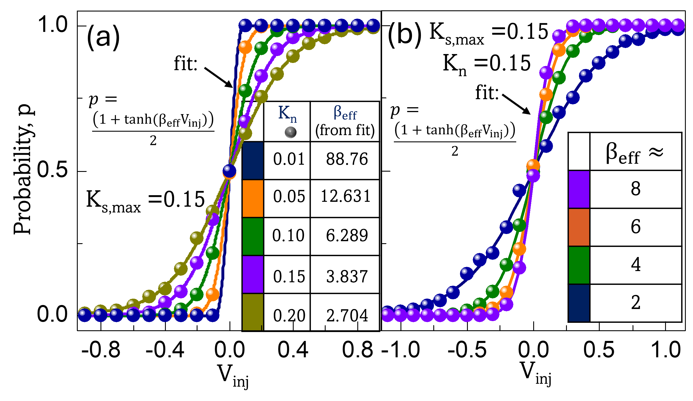
The image contains two panels (a) and (b) depicting probability distributions as a function of injected voltage (V_inj). Both panels include:
- Sigmoidal curves fitted with the equation:
$ p = \frac{1 + \tanh(\beta_{\text{eff}} V_{\text{inj}})}{2} $
- Tables listing numerical parameters (K_n, β_eff)
- Legends mapping colors to K_n values
- Key annotations for maximum curvature (K_s,max) and fit parameters
### Components/Axes
#### Panel (a)
- **X-axis**: V_inj (ranging from -0.8 to 1.0)
- **Y-axis**: Probability, p (0.0 to 1.0)
- **Legend**: Located at top-right, colors correspond to K_n values (0.01, 0.05, 0.10, 0.15, 0.20)
- **Fit Equation**: Annotated with $ K_{s,\text{max}} = 0.15 $
- **Table**: Embedded in the plot, showing K_n and β_eff values:
| K_n | β_eff (from fit) |
|-------|------------------|
| 0.01 | 88.76 |
| 0.05 | 12.631 |
| 0.10 | 6.289 |
| 0.15 | 3.837 |
| 0.20 | 2.704 |
#### Panel (b)
- **X-axis**: V_inj (ranging from -1.0 to 1.0)
- **Y-axis**: Probability, p (0.0 to 1.0)
- **Legend**: Located at top-right, colors correspond to β_eff ≈ 8, 6, 4, 2
- **Fit Equation**: Annotated with $ K_{s,\text{max}} = 0.15 $, $ K_n = 0.15 $
- **Table**: Embedded in the plot, showing β_eff approximations:
| β_eff ≈ | Color |
|---------|--------|
| 8 | Purple |
| 6 | Orange |
| 4 | Green |
| 2 | Blue |
### Detailed Analysis
#### Panel (a)
- **Curves**: Five sigmoidal curves (dark blue to olive green) represent increasing K_n values. Higher K_n curves are steeper and shift rightward.
- **Fit Equation**: The tanh function models probability as a function of V_inj, with β_eff inversely proportional to K_n (e.g., β_eff = 88.76 for K_n = 0.01 vs. 2.704 for K_n = 0.20).
- **K_s,max**: Annotated at V_inj = -0.15, indicating the voltage at maximum curvature for all curves.
#### Panel (b)
- **Curves**: Four sigmoidal curves (purple to dark blue) represent decreasing β_eff values. Lower β_eff curves are shallower and shift leftward.
- **Fit Equation**: Same tanh form as panel (a), but β_eff is fixed at ≈8, 6, 4, 2, with K_n = 0.15 constant.
- **K_s,max**: Same value (0.15) as panel (a), but curves are less steep due to fixed K_n.
### Key Observations
1. **Inverse Relationship**: Higher K_n values (panel a) correlate with lower β_eff, reducing the sensitivity of probability to V_inj.
2. **Steepness vs. Spread**: Panel (a) shows steeper curves for smaller K_n, while panel (b) shows broader distributions for lower β_eff.
3. **Consistency**: Both panels use the same fit equation, but panel (b) fixes K_n = 0.15, altering the parameter space.
4. **Color-Legend Matching**: All curves in both panels align with their respective legend colors (e.g., dark blue = K_n = 0.20 in panel a; purple = β_eff ≈8 in panel b).
### Interpretation
The data demonstrates how probability distributions of an injected voltage-dependent process are modulated by two parameters:
1. **K_n**: Controls the steepness of the sigmoidal curve. Smaller K_n values (e.g., 0.01) produce sharper transitions, while larger K_n (e.g., 0.20) yield broader distributions.
2. **β_eff**: Represents the effective voltage sensitivity. Higher β_eff (e.g., 88.76) amplifies the effect of V_inj, whereas lower β_eff (e.g., 2.704) dampens it.
The fit equation $ p = \frac{1 + \tanh(\beta_{\text{eff}} V_{\text{inj}})}{2} $ suggests a logistic-like behavior, where probability transitions from 0 to 1 as V_inj crosses zero. The tables confirm that β_eff scales inversely with K_n (panel a) and is discretized in panel (b). The consistent K_s,max = 0.15 across panels implies a universal curvature point, independent of K_n or β_eff. This could reflect a physical constraint (e.g., maximum response rate) in the system being modeled.