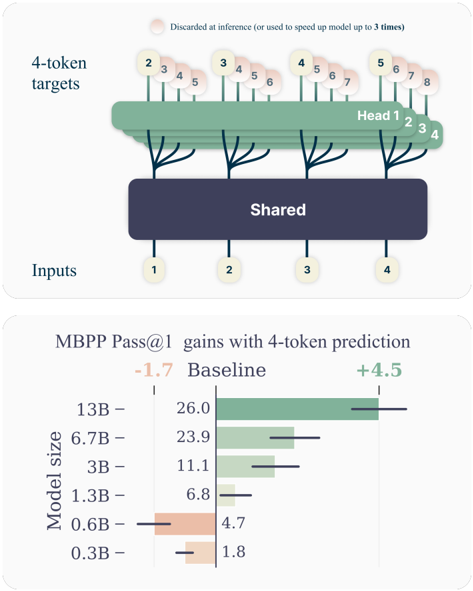
## Diagram and Chart: 4-Token Prediction Architecture and Performance Gains ### Overview The image contains two distinct but related technical illustrations. The top section is a schematic diagram of a neural network architecture designed for 4-token prediction. The bottom section is a horizontal bar chart quantifying the performance gains (in MBPP Pass@1 score) achieved by this method across different model sizes, compared to a baseline. ### Components/Axes **Top Diagram: Architecture Schematic** * **Inputs:** A row of four circular nodes at the bottom, labeled sequentially: `1`, `2`, `3`, `4`. * **Shared Layer:** A large, dark blue rectangular block labeled `Shared` in white text. It receives connections from all four input nodes. * **Heads:** Four distinct green, tree-like structures emerging from the top of the `Shared` block. They are labeled `Head 1`, `Head 2`, `Head 3`, `Head 4` from left to right. * **4-token targets:** A row of circular nodes at the top, grouped in sets of four corresponding to each head. The groups are: * Head 1 targets: `2`, `3`, `4`, `5` * Head 2 targets: `3`, `4`, `5`, `6` * Head 3 targets: `4`, `5`, `6`, `7` * Head 4 targets: `5`, `6`, `7`, `8` * **Annotation:** A text note at the very top reads: `Discarded at inference (or used to speed up model up to 3 times)`. A faint, pinkish circular highlight is placed over the first token (`2`) of the first target group. **Bottom Chart: MBPP Pass@1 Gains** * **Title:** `MBPP Pass@1 gains with 4-token prediction` * **Y-axis (Vertical):** Labeled `Model size`. Categories from top to bottom: `13B`, `6.7B`, `3B`, `1.3B`, `0.6B`, `0.3B`. * **X-axis (Horizontal):** Represents the MBPP Pass@1 score. A central vertical line marks the `Baseline` score for each model. * **Legend/Key:** Located at the top of the chart area. * `-1.7` in orange text, associated with a leftward (negative) bar. * `Baseline` in black text, associated with the central vertical line. * `+4.5` in green text, associated with a rightward (positive) bar. * **Data Series:** For each model size, a horizontal bar shows the change from the baseline. * **Baseline Values (black text, left of center line):** * 13B: `26.0` * 6.7B: `23.9` * 3B: `11.1` * 1.3B: `6.8` * 0.6B: `4.7` * 0.3B: `1.8` * **Gain/Loss Bars (colored, extending from baseline):** * **13B:** A long green bar extending to the right. The gain is approximately `+4.5` (matching the legend's maximum). * **6.7B:** A green bar extending to the right. Gain is approximately `+2.5` to `+3.0`. * **3B:** A green bar extending to the right. Gain is approximately `+1.5` to `+2.0`. * **1.3B:** A very short green bar extending to the right. Gain is approximately `+0.5`. * **0.6B:** An orange bar extending to the left. Loss is approximately `-1.0` to `-1.5`. * **0.3B:** A very short orange bar extending to the left. Loss is approximately `-0.2` to `-0.5`. ### Detailed Analysis **Architecture Diagram Flow:** The diagram illustrates a "shared trunk, multiple heads" architecture for next-token prediction. The four input tokens (`1-4`) are processed by a common `Shared` representation layer. From this shared representation, four separate prediction heads (`Head 1-4`) are instantiated. Each head is responsible for predicting a different, overlapping sequence of four future tokens. For example, Head 1 predicts tokens 2, 3, 4, 5, while Head 2 predicts tokens 3, 4, 5, 6. The annotation suggests that the predictions from these specialized heads (or parts of them) are not used during standard inference but can be leveraged to accelerate the model, potentially by a factor of up to 3. **Chart Data Trends:** The chart demonstrates a clear, positive correlation between model size and the effectiveness of the 4-token prediction method. * **Trend Verification:** The green bars (gains) grow progressively longer as model size increases from 1.3B to 13B. Conversely, the smallest models (0.6B and 0.3B) show negative gains (orange bars), indicating a performance regression. * **Key Data Points:** The largest model (13B) achieves the maximum illustrated gain of +4.5 points over its strong baseline of 26.0. The 6.7B model shows a substantial gain of ~+2.75. The method becomes detrimental for models at or below 0.6B parameters. ### Key Observations 1. **Scale-Dependent Efficacy:** The 4-token prediction technique is not universally beneficial. It provides significant gains for medium to large models (1.3B and above) but harms the performance of very small models (0.6B and below). 2. **Architecture Specificity:** The diagram shows a precise, non-autoregressive prediction pattern where each head predicts a fixed-length window of future tokens, differing from standard single-token next-prediction. 3. **Performance Ceiling:** The gain for the 13B model (+4.5) is explicitly called out in the legend, suggesting it might be a target or observed maximum in the experiment. 4. **Inference Optimization Hint:** The note about discarding predictions or using them for speed hints that this architecture is designed for efficiency, possibly enabling speculative decoding or parallel token generation. ### Interpretation This image presents a method to improve code generation performance (as measured by the MBPP benchmark) by modifying a language model's prediction objective. Instead of predicting one next token, the model is trained with specialized heads to predict four future tokens simultaneously from a shared representation. The data suggests this approach forces the model to learn more robust and forward-looking representations, which benefits larger models that have the capacity to leverage this complex objective. For small models, the added complexity of predicting multiple future tokens may be overwhelming, leading to worse performance than the simpler baseline. The architectural diagram explains the "how," while the performance chart validates the "why" and "for whom." The combined message is that this 4-token prediction is a promising technique for scaling up the efficiency and capability of larger language models, particularly for tasks like code generation where understanding longer-range structure is crucial. The inference speed-up note further positions it as a practical optimization for deployment.