## Diagram: Constrained BFS-Tree Transformation
### Overview
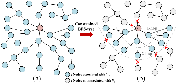
The image is a technical diagram illustrating the transformation of a network graph into a "Constrained BFS-tree." It consists of two network graphs, labeled (a) and (b), connected by a red arrow indicating the transformation process. The diagram visually explains how a Breadth-First Search (BFS) tree is constructed from a root node under specific constraints, limiting the included nodes based on hop distance and association.
### Components/Axes
* **Main Elements:** Two network graphs, (a) and (b), positioned side-by-side.
* **Transformation Arrow:** A thick red arrow points from graph (a) to graph (b). Above the arrow is the text "Constrained BFS-tree".
* **Node Legend:** Located at the bottom center of the image.
* A light blue circle is labeled: "Nodes associated with \( v_r \)"
* A white circle is labeled: "Nodes not associated with \( v_r \)"
* **Graph Labels:**
* The central root node in both graphs is labeled \( v_r \) and is colored pink.
* In graph (b), two dashed, concentric arcs are drawn around \( v_r \). The inner arc is labeled "1-hop" and the outer arc is labeled "2-hop".
* **Annotations in Graph (b):** Several red "X" marks are placed on specific edges (connections between nodes).
### Detailed Analysis
**Graph (a) - Initial State:**
* **Structure:** A star-like network with the pink root node \( v_r \) at the center-left.
* **Nodes:** All nodes surrounding \( v_r \) are light blue. According to the legend, this means every node in this graph is "associated with \( v_r \)."
* **Edges:** Solid black lines connect \( v_r \) to its immediate neighbors and connect those neighbors to other nodes, forming a connected network.
**Graph (b) - Constrained BFS-tree Result:**
* **Structure:** The same spatial layout of nodes as in (a), but with critical changes in node association and edge validity.
* **Node Association Changes:**
* Nodes located within the "2-hop" dashed arc (including those within the "1-hop" arc) remain light blue ("associated").
* Nodes located outside the "2-hop" arc have changed from light blue to white ("not associated").
* **Edge Annotations (Red 'X' marks):** Red crosses are placed on edges that connect:
1. A light blue node (inside 2-hop) to a white node (outside 2-hop).
2. Two white nodes (both outside 2-hop).
* This visually indicates that these edges are excluded or constrained in the resulting BFS-tree.
* **Implied Flow:** The transformation shows a selection process. The BFS algorithm, starting from \( v_r \), includes nodes only up to a 2-hop distance (or based on another association metric), creating a subtree. Nodes and edges beyond this constraint are marked as excluded.
### Key Observations
1. **Hop-Based Constraint:** The primary constraint visualized is distance from the root. The "1-hop" and "2-hop" arcs explicitly define the boundary for node inclusion.
2. **Association vs. Distance:** The legend defines nodes as "associated" or "not associated." In graph (b), association perfectly correlates with being within the 2-hop boundary, suggesting the constraint is based on hop count.
3. **Edge Pruning:** The red 'X' marks demonstrate that the constrained tree is formed not just by selecting nodes, but by pruning specific connecting edges that violate the constraint rules.
4. **Spatial Consistency:** The physical positions of all nodes are identical between (a) and (b), allowing for direct visual comparison of the state changes.
### Interpretation
This diagram is a pedagogical tool explaining a **constrained graph traversal algorithm**. It demonstrates how a standard BFS exploration from a root node (\( v_r \)) can be limited by a specific rule—in this case, a maximum hop distance of 2.
* **What it shows:** The process transforms a fully associated network (a) into a pruned subtree (b). The subtree includes only nodes deemed "associated" (within 2 hops), and the edges connecting them. All other nodes and their connecting edges are marked as excluded.
* **Why it matters:** In real-world networks (social, communication, biological), unconstrained BFS can be computationally expensive or include irrelevant nodes. Constraints like hop limit, node attribute ("association"), or edge weight are essential for efficient and meaningful analysis. This diagram makes the abstract concept of a constrained search concrete.
* **Underlying Logic:** The red 'X's are crucial. They show that the algorithm doesn't just stop at the 2-hop boundary; it actively identifies and disregards the links that would lead outside the constrained set, formally defining the edges of the resulting BFS-tree. The perfect alignment of "association" with the 2-hop zone in this example suggests the constraint is purely topological (distance-based), but the framework could accommodate other association criteria.