## Combination Chart: Performance Metrics vs. Graph-Constrained Decoding Beam Size
### Overview
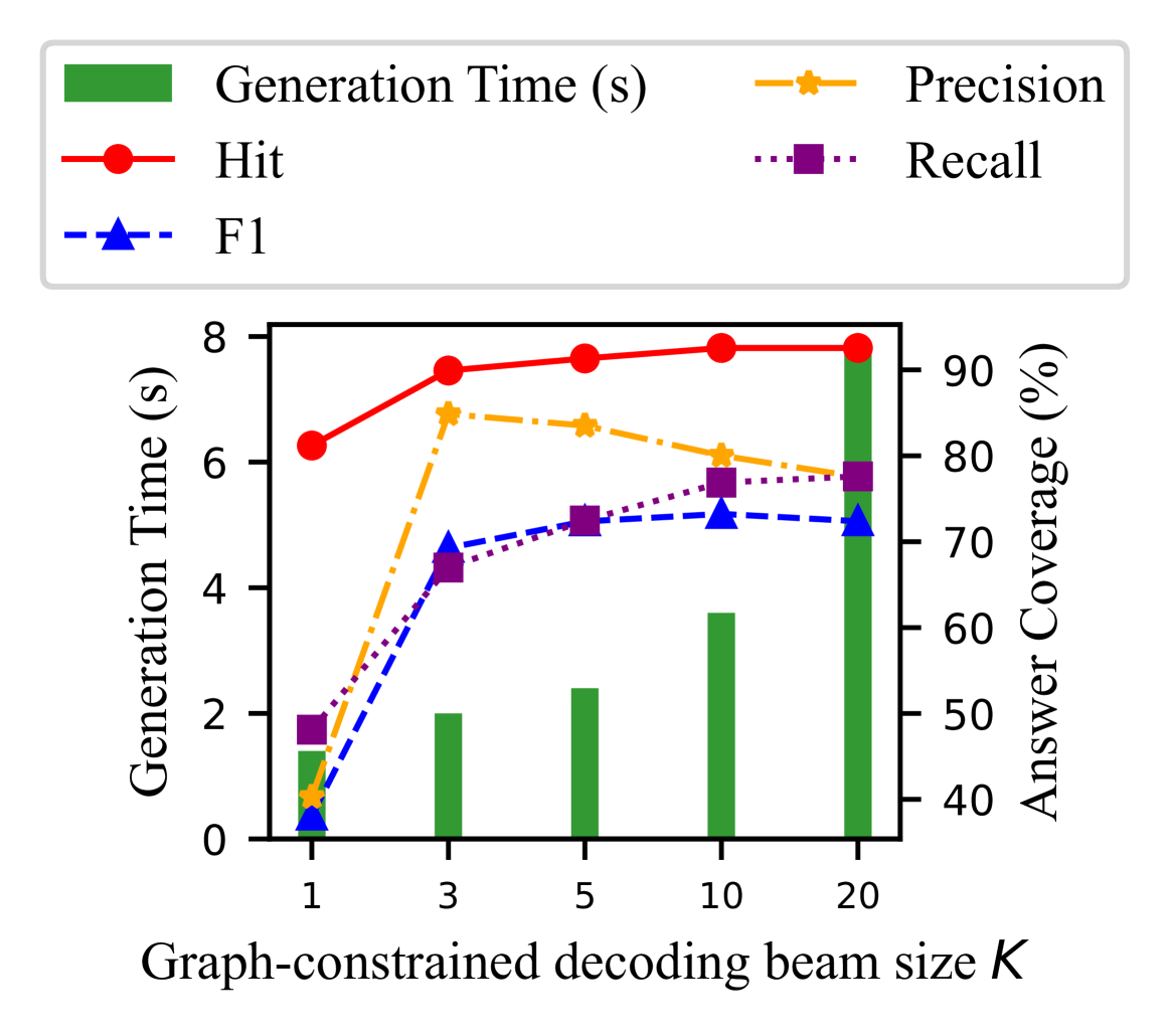
This image is.......... The chart uses a dual y-axis: the left axis measures time in seconds, and the right axis measures percentage-based coverage metrics. The data demonstrates the trade-offs between computational cost (time) and answer quality (coverage) as the beam search parameter `K` increases.
### Components/Axes
* **X-Axis (Bottom):** Labeled "Graph-constrained decoding beam size K". It has five discrete, non-linearly spaced tick marks at values: `1`, `3`, `5`, `10`, and `20`.
* **Primary Y-Axis (Left):** Labeled "Generation Time (s)". Scale runs from 0 to 8 with major ticks at intervals of 2 (0, 2, 4, 6, 8).
* **Secondary Y-Axis (Right):** Labeled "Answer Coverage (%)". Scale runs from 40 to 90 with major ticks at intervals of 10 (40, 50, 60, 70, 80, 90).
* **Legend (Top, Centered):** Contains five entries, each with a distinct color, line style, and marker:
1. **Generation Time (s):** Represented by a solid green bar.
2. **Hit:** Represented by a solid red line with circular markers.
3. **F1:** Represented by a blue dashed line with upward-pointing triangle markers.
4. **Precision:** Represented by an orange dash-dot line with star/asterisk markers.
5. **Recall:** Represented by a purple dotted line with square markers.
### Detailed Analysis
The chart displays data for each beam size `K` as follows. Values are approximate visual estimates.
**Trend Verification & Data Points:**
* **Generation Time (Green Bars):** Shows a clear, monotonic upward trend. Time cost increases significantly with beam size.
* K=1: ~1.3 seconds
* K=3: ~2.0 seconds
* K=5: ~2.4 seconds
* K=10: ~3.6 seconds
* K=20: ~7.8 seconds
* **Hit (Red Line, Circles):** Increases sharply from K=1 to K=3, then plateaus, showing very slight growth thereafter.
* K=1: ~82%
* K=3: ~89%
* K=5: ~90%
* K=10: ~91%
* K=20: ~91%
* **Precision (Orange Line, Stars):** Increases sharply from K=1 to K=3, then begins a gradual decline.
* K=1: ~42%
* K=3: ~85%
* K=5: ~83%
* K=10: ~80%
* K=20: ~78%
* **Recall (Purple Line, Squares):** Shows a steady, monotonic increase across all beam sizes.
* K=1: ~49%
* K=3: ~66%
* K=5: ~72%
* K=10: ~77%
* K=20: ~78%
* **F1 (Blue Line, Triangles):** Follows a similar pattern to Precision but with a lower peak and a more stable plateau after K=3.
* K=1: ~40%
* K=3: ~70%
* K=5: ~72%
* K=10: ~73%
* K=20: ~72%
### Key Observations
1. **Diminishing Returns:** After `K=3`, the gains in Hit rate, F1, and Recall become marginal, while Precision starts to decrease.
2. **Cost vs. Benefit:** The most dramatic improvements in all coverage metrics occur when increasing `K` from 1 to 3. The generation time, however, continues to grow substantially beyond this point, especially at `K=20`.
3. **Precision-Recall Trade-off:** The chart visually captures the classic trade-off. As `K` increases, Recall steadily improves, but Precision peaks early (`K=3`) and then declines, suggesting the model retrieves more relevant answers but also introduces more noise at higher beam sizes.
4. **F1 Score Stability:** The F1 score, which balances Precision and Recall, stabilizes around 72-73% for `K >= 3`, indicating that further increases in beam size do not improve the overall harmonic mean of precision and recall.
### Interpretation
This chart illustrates a critical optimization problem in machine learning model decoding, likely for a question-answering or generation task using a graph-based constraint. The parameter `K` (beam size) controls the breadth of the search during decoding.
* **What the data suggests:** A small beam size (`K=1`) is fast but yields poor coverage. Increasing the beam size to `K=3` provides a substantial boost to all quality metrics (Hit, Precision, Recall, F1) for a moderate time increase. This appears to be the "sweet spot" or optimal operating point for efficiency.
* **Why it matters:** Beyond `K=3`, the system enters a zone of diminishing returns. The computational cost (Generation Time) escalates, particularly at `K=20`, while the primary quality metric (Hit rate) barely improves. The decline in Precision suggests that a wider search starts incorporating less relevant or incorrect paths from the graph constraint.
* **Underlying Pattern:** The data demonstrates that more exhaustive search (higher `K`) does not linearly translate to better performance. There is an optimal complexity threshold (`K=3` in this case) after which the cost outweighs the benefits, and the model's output may become less precise. This is a fundamental insight for deploying such systems in resource-constrained or real-time environments.