## Diagram: Probabilistic Inference Steps ### Overview The image presents a diagram illustrating a three-step process for probabilistic inference. The steps involve learning a posterior weight space, sampling from the weight posterior, and performing predictive posterior inference. The diagram uses visual representations and mathematical notation to describe each step. ### Components/Axes * **Step 1:** Learning Posterior Weight Space * Visual: A 3D mesh plot representing the weight space. A blue dot is highlighted on the surface. * Text: p(W_EC|D) ∝ p(D|W_EC)p(W_EC) * **Step 2:** Sampling from Weight Posterior * Visual: A color-coded matrix, with each column representing a sample. The matrix is labeled "x S" at the top. * Text: W^s_EC ~ p(W_EC|D) * **Hidden Token Input:** * Visual: A box labeled "Hidden Token Input u" with an arrow pointing to Step 3. * **Step 3:** Predictive Posterior Inference * Visual: A mathematical equation. * Text: s = (1/S) Σ_s=1^S softmax(u W^s_EC) ### Detailed Analysis * **Step 1:** The 3D mesh plot in Step 1 visually represents the posterior weight space. The blue dot indicates a specific point within this space. The equation p(W_EC|D) ∝ p(D|W_EC)p(W_EC) describes the relationship between the posterior probability of the weights given the data (W_EC|D), the likelihood of the data given the weights (D|W_EC), and the prior probability of the weights (W_EC). * **Step 2:** The color-coded matrix in Step 2 represents samples drawn from the weight posterior. Each column represents a sample (S samples in total). The equation W^s_EC ~ p(W_EC|D) indicates that the samples W^s_EC are drawn from the posterior distribution p(W_EC|D). * **Hidden Token Input:** The "Hidden Token Input u" represents an input vector that is used in the predictive posterior inference step. * **Step 3:** The equation s = (1/S) Σ_s=1^S softmax(u W^s_EC) in Step 3 describes the predictive posterior inference process. It calculates the weighted average of the softmax function applied to the product of the input vector u and each sample W^s_EC. ### Key Observations * The diagram illustrates a sequential process, with each step building upon the previous one. * The diagram combines visual representations (3D plot, color-coded matrix) with mathematical notation to describe the probabilistic inference process. * The "Hidden Token Input" acts as an external input to the inference process. ### Interpretation The diagram provides a high-level overview of a probabilistic inference method. It shows how to learn a posterior weight space, sample from it, and use the samples to make predictions. The use of a "Hidden Token Input" suggests that this method is likely used in a context where external information is available and can be incorporated into the inference process. The softmax function in Step 3 suggests that the output is a probability distribution. The diagram demonstrates a Bayesian approach to inference, where prior knowledge (represented by the prior probability of the weights) is combined with data to obtain a posterior distribution, which is then used to make predictions.

\n ## Diagram: Predictive Posterior Inference Process ### Overview The image depicts a three-step process for predictive posterior inference. It illustrates a flow from learning a posterior weight space, sampling from that space, and finally performing predictive posterior inference. The diagram uses visual representations of mathematical concepts and equations to explain the process. ### Components/Axes The diagram is divided into three main steps, labeled "Step 1", "Step 2", and "Step 3", arranged horizontally from left to right. Each step has a descriptive title and a corresponding visual representation. * **Step 1: Learning Posterior Weight Space:** Visualized as a 3D surface plot with two blue dots on the surface. The equation below it is: `p(WEC|D) ∝ p(D|WEC)p(WEC)` * **Step 2: Sampling from Weight Posterior:** Represented as a grid of colored rectangles (S x S). The equation below it is: `WEC ~ p(WEC|D)` * **Step 3: Predictive Posterior Inference:** Shown as a box with an arrow pointing into it. The equation within the box is: `s = 1/S ∑ softmax(u WEC)` where the summation is from s=1 to S. * **Hidden Token Input:** Labeled as "Hidden Token Input" and represented as a vertical arrow pointing towards Step 3. The variable is denoted as "u". * **S:** Appears in the equations for Step 2 and Step 3, representing a dimension or size parameter. ### Detailed Analysis or Content Details **Step 1:** The 3D surface plot represents a probability distribution over weights (WEC) given data (D). The two blue dots likely represent specific weight values sampled from this distribution. The equation indicates that the posterior probability of the weights given the data is proportional to the likelihood of the data given the weights multiplied by the prior probability of the weights. **Step 2:** The grid of colored rectangles represents sampling from the posterior weight distribution. The dimensions of the grid are S x S. The equation indicates that a weight vector (WEC) is sampled from the posterior distribution p(WEC|D). The colors of the rectangles are varied, suggesting different sampled weight values. **Step 3:** This step performs predictive inference using the sampled weights. The equation calculates a prediction 's' as the average of the softmax of the product of the hidden token input 'u' and each sampled weight vector WEC. The summation is performed over S samples. ### Key Observations * The diagram illustrates a Bayesian approach to inference, where uncertainty is represented by a probability distribution over weights. * The sampling step (Step 2) is crucial for approximating the posterior predictive distribution. * The final prediction (Step 3) is a weighted average of the softmax outputs, where the weights are determined by the sampled weights. * The variable 'S' appears to represent the number of samples used in the Monte Carlo approximation. ### Interpretation The diagram describes a method for making predictions based on a Bayesian model. The process begins by learning a posterior distribution over the model's weights given the observed data. This posterior distribution represents our uncertainty about the true values of the weights. To make a prediction, we sample multiple weight vectors from this posterior distribution and average the predictions made by each weight vector. This averaging process effectively integrates over the uncertainty in the weights, resulting in a more robust and accurate prediction. The use of the softmax function suggests that the model is making predictions about a categorical variable. The "Hidden Token Input" (u) likely represents a feature vector or embedding of the input data. The diagram highlights the importance of representing uncertainty and using sampling techniques to approximate complex distributions. The diagram is a conceptual illustration of a Bayesian inference process, and does not contain specific numerical data.

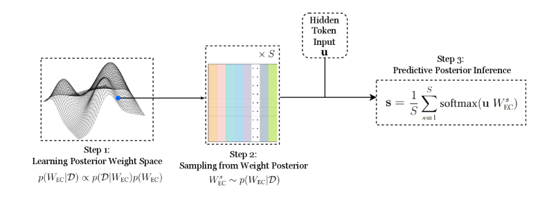
## Diagram: Three-Step Process for Predictive Posterior Inference ### Overview The image is a technical diagram illustrating a three-step computational process, likely for Bayesian inference or uncertainty estimation in a machine learning model. The flow moves from left to right, starting with learning a weight distribution, sampling from it, and finally using those samples to make a prediction. The diagram combines graphical representations, mathematical notation, and text labels. ### Components/Axes The diagram is segmented into three primary components, connected by directional arrows indicating the flow of data or process. 1. **Step 1: Learning Posterior Weight Space** (Leftmost box) * **Visual:** A 3D wireframe surface plot with multiple peaks and valleys, representing a complex probability distribution. A single blue dot is placed on one of the slopes. * **Text Label:** "Step 1: Learning Posterior Weight Space" * **Mathematical Notation:** `p(W_EC|D) ∝ p(D|W_EC)p(W_EC)` * **Spatial Position:** Located on the far left of the diagram. 2. **Step 2: Sampling from Weight Posterior** (Central box) * **Visual:** A rectangular block divided into multiple vertical columns of different colors (from left to right: orange, light blue, purple, grey, green). The notation "× S" is placed above the top-right corner of this block. * **Text Label:** "Step 2: Sampling from Weight Posterior" * **Mathematical Notation:** `W_EC^s ~ p(W_EC|D)` * **Spatial Position:** Centered in the diagram, receiving an arrow from Step 1. 3. **Step 3: Predictive Posterior Inference** (Rightmost box) * **Visual:** A rectangular box containing a mathematical formula. * **Text Label:** "Step 3: Predictive Posterior Inference" * **Mathematical Notation:** `s = (1/S) * Σ_{s=1}^{S} softmax(u W_EC^s)` * **Spatial Position:** Located on the far right of the diagram. 4. **Hidden Token Input** (Top-center box) * **Visual:** A dashed-line box containing text. * **Text Label:** "Hidden Token Input u" * **Spatial Position:** Positioned above the arrow connecting Step 2 to Step 3, indicating it is an input to the final step. ### Detailed Analysis The process is defined by the following sequence and relationships: * **Flow Direction:** The process flows unidirectionally from Step 1 → Step 2 → Step 3. An additional input (`u`) is introduced between Step 2 and Step 3. * **Step 1 Details:** This step represents the training or fitting phase. The formula `p(W_EC|D) ∝ p(D|W_EC)p(W_EC)` is Bayes' theorem, indicating the model is learning the posterior distribution of weights (`W_EC`) given some data (`D`). The 3D plot visually represents this complex, multi-modal posterior distribution. * **Step 2 Details:** This step involves generating `S` samples from the learned posterior distribution. The colored block represents a collection of `S` weight matrices or vectors (`W_EC^s`), where each color likely corresponds to a different sample `s`. The notation `~` means "sampled from." * **Step 3 Details:** This is the inference or prediction phase. For a given input (the "Hidden Token Input u"), the model computes a prediction `s`. This is done by: 1. Taking each of the `S` weight samples (`W_EC^s`) from Step 2. 2. Computing the softmax of the product `u * W_EC^s` for each sample. 3. Averaging these `S` softmax outputs (the `(1/S) * Σ` operation). * **Input `u`:** The "Hidden Token Input u" is a vector or matrix that is multiplied by each sampled weight matrix `W_EC^s` before the softmax function is applied. ### Key Observations * The diagram explicitly models **uncertainty** by using a distribution over weights (`p(W_EC|D)`) rather than a single point estimate. * The final prediction `s` is an **ensemble average** over `S` different models, each parameterized by a weight sample from the posterior. This is a common technique for Bayesian neural networks or Monte Carlo dropout. * The use of the **softmax** function in Step 3 suggests the final output `s` is a probability distribution over classes (e.g., for a classification task). * The visual metaphor in Step 1 (a complex landscape) effectively communicates the idea of a high-dimensional, non-convex posterior distribution that is difficult to characterize with a simple formula. ### Interpretation This diagram outlines a **Bayesian neural network inference pipeline**. The core idea is to move beyond a single "best guess" model and instead maintain a probability distribution over all plausible models (weights) that fit the training data. 1. **Learning (Step 1):** The model doesn't just find one set of optimal weights; it learns the entire landscape of probable weights. The blue dot on the surface may represent a maximum a posteriori (MAP) estimate, but the process considers the whole distribution. 2. **Sampling (Step 2):** To make this intractable distribution usable, the model draws a finite number (`S`) of representative weight configurations. Each colored column is a different "version" of the model. 3. **Prediction (Step 3):** When presented with new data (`u`), each version of the model makes its own prediction (via `softmax(u W_EC^s)`). The final output is the average of all these predictions. This averaging smooths out the idiosyncrasies of any single weight sample, leading to a more robust and calibrated prediction that inherently quantifies uncertainty. A high variance among the individual `softmax` outputs would indicate high model uncertainty for that input. **In essence, the diagram shows how to transform a complex, learned probability distribution over model parameters into a practical, averaged prediction for new data, providing a principled way to handle uncertainty in machine learning.**

## Flowchart: Bayesian Neural Network Inference Process ### Overview The diagram illustrates a three-step Bayesian inference process for neural network prediction, combining probabilistic modeling with predictive inference. It visualizes weight space learning, posterior sampling, and predictive aggregation. ### Components/Axes 1. **Step 1: Learning Posterior Weight Space** - Equation: `p(W_EC|D) ∝ p(D|W_EC)p(W_EC)` - Visual: 3D surface plot with blue point indicating optimal weight configuration - Axes: Implicit weight dimensions (W_EC) vs. probability density 2. **Step 2: Sampling from Weight Posterior** - Equation: `W_EC^s ~ p(W_EC|D)` - Visual: Color-coded bars (orange, blue, green) representing sampled weights - Input: Hidden token `u` (rectangular box with dashed border) 3. **Step 3: Predictive Posterior Inference** - Equation: `s = 1/S Σ softmax(u W_EC^s)` - Visual: Final output box with summation notation - Output: Predictive distribution `s` ### Detailed Analysis - **Step 1** shows a posterior distribution landscape where the blue point represents maximum a posteriori (MAP) estimates. The surface plot suggests multimodal weight configurations. - **Step 2** depicts stochastic sampling from the learned posterior, with three distinct weight configurations (orange/blue/green bars) drawn from `p(W_EC|D)`. - **Step 3** combines sampled weights with hidden input `u` through softmax normalization, producing a predictive distribution averaged over `S` samples. ### Key Observations 1. The blue point in Step 1's surface plot corresponds to the highest probability density region in the posterior distribution. 2. Step 2's color-coded bars maintain consistent width but vary in height, indicating different probability densities for each sampled weight configuration. 3. The predictive inference equation in Step 3 shows ensemble averaging over softmax-transformed weight-input products. ### Interpretation This diagram demonstrates Bayesian neural network inference through: 1. **Probabilistic Modeling**: Step 1 combines likelihood (`p(D|W_EC)`) and prior (`p(W_EC)`) to form posterior distributions 2. **Stochastic Approximation**: Step 2 samples from the posterior rather than using point estimates, capturing uncertainty 3. **Predictive Aggregation**: Step 3 combines multiple weight configurations through softmax normalization, effectively performing Bayesian model averaging The process reflects Bayesian inference principles where: - Weight space learning incorporates prior knowledge - Posterior sampling accounts for model uncertainty - Predictive inference aggregates over multiple hypotheses (weight configurations) The blue point in Step 1's surface plot suggests the model identifies a dominant weight configuration, while Step 2's sampling acknowledges potential multimodality. The final predictive distribution in Step 3 represents a consensus over sampled hypotheses, typical of Bayesian neural network approaches.