## Diagram: Probabilistic Inference Steps
### Overview
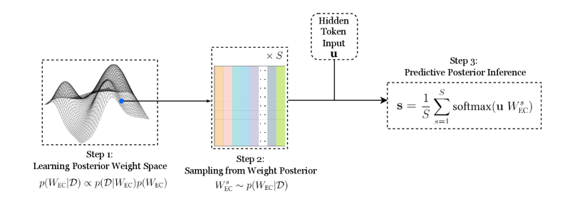
The image presents a diagram illustrating a three-step process for probabilistic inference. The steps involve learning a posterior weight space, sampling from the weight posterior, and performing predictive posterior inference. The diagram uses visual representations and mathematical notation to describe each step.
### Components/Axes
* **Step 1:** Learning Posterior Weight Space
* Visual: A 3D mesh plot representing the weight space. A blue dot is highlighted on the surface.
* Text: p(W<sub>EC</sub>|D) ∝ p(D|W<sub>EC</sub>)p(W<sub>EC</sub>)
* **Step 2:** Sampling from Weight Posterior
* Visual: A color-coded matrix, with each column representing a sample. The matrix is labeled "x S" at the top.
* Text: W<sup>s</sup><sub>EC</sub> ~ p(W<sub>EC</sub>|D)
* **Hidden Token Input:**
* Visual: A box labeled "Hidden Token Input u" with an arrow pointing to Step 3.
* **Step 3:** Predictive Posterior Inference
* Visual: A mathematical equation.
* Text: s = (1/S) Σ<sub>s=1</sub><sup>S</sup> softmax(u W<sup>s</sup><sub>EC</sub>)
### Detailed Analysis
* **Step 1:** The 3D mesh plot in Step 1 visually represents the posterior weight space. The blue dot indicates a specific point within this space. The equation p(W<sub>EC</sub>|D) ∝ p(D|W<sub>EC</sub>)p(W<sub>EC</sub>) describes the relationship between the posterior probability of the weights given the data (W<sub>EC</sub>|D), the likelihood of the data given the weights (D|W<sub>EC</sub>), and the prior probability of the weights (W<sub>EC</sub>).
* **Step 2:** The color-coded matrix in Step 2 represents samples drawn from the weight posterior. Each column represents a sample (S samples in total). The equation W<sup>s</sup><sub>EC</sub> ~ p(W<sub>EC</sub>|D) indicates that the samples W<sup>s</sup><sub>EC</sub> are drawn from the posterior distribution p(W<sub>EC</sub>|D).
* **Hidden Token Input:** The "Hidden Token Input u" represents an input vector that is used in the predictive posterior inference step.
* **Step 3:** The equation s = (1/S) Σ<sub>s=1</sub><sup>S</sup> softmax(u W<sup>s</sup><sub>EC</sub>) in Step 3 describes the predictive posterior inference process. It calculates the weighted average of the softmax function applied to the product of the input vector u and each sample W<sup>s</sup><sub>EC</sub>.
### Key Observations
* The diagram illustrates a sequential process, with each step building upon the previous one.
* The diagram combines visual representations (3D plot, color-coded matrix) with mathematical notation to describe the probabilistic inference process.
* The "Hidden Token Input" acts as an external input to the inference process.
### Interpretation
The diagram provides a high-level overview of a probabilistic inference method. It shows how to learn a posterior weight space, sample from it, and use the samples to make predictions. The use of a "Hidden Token Input" suggests that this method is likely used in a context where external information is available and can be incorporated into the inference process. The softmax function in Step 3 suggests that the output is a probability distribution. The diagram demonstrates a Bayesian approach to inference, where prior knowledge (represented by the prior probability of the weights) is combined with data to obtain a posterior distribution, which is then used to make predictions.