## Flowchart: Bayesian Neural Network Inference Process
### Overview
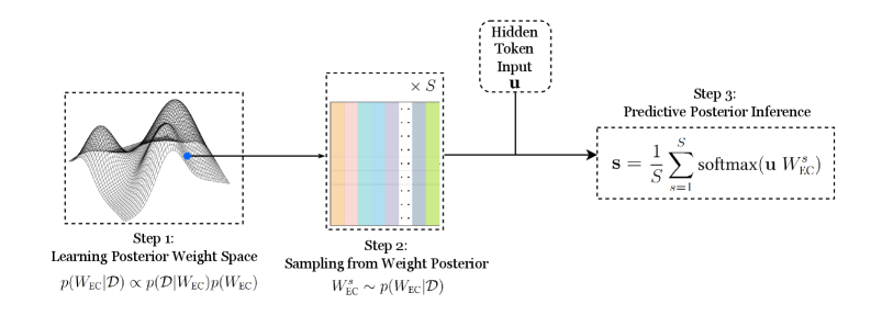
The diagram illustrates a three-step Bayesian inference process for neural network prediction, combining probabilistic modeling with predictive inference. It visualizes weight space learning, posterior sampling, and predictive aggregation.
### Components/Axes
1. **Step 1: Learning Posterior Weight Space**
- Equation: `p(W_EC|D) ∝ p(D|W_EC)p(W_EC)`
- Visual: 3D surface plot with blue point indicating optimal weight configuration
- Axes: Implicit weight dimensions (W_EC) vs. probability density
2. **Step 2: Sampling from Weight Posterior**
- Equation: `W_EC^s ~ p(W_EC|D)`
- Visual: Color-coded bars (orange, blue, green) representing sampled weights
- Input: Hidden token `u` (rectangular box with dashed border)
3. **Step 3: Predictive Posterior Inference**
- Equation: `s = 1/S Σ softmax(u W_EC^s)`
- Visual: Final output box with summation notation
- Output: Predictive distribution `s`
### Detailed Analysis
- **Step 1** shows a posterior distribution landscape where the blue point represents maximum a posteriori (MAP) estimates. The surface plot suggests multimodal weight configurations.
- **Step 2** depicts stochastic sampling from the learned posterior, with three distinct weight configurations (orange/blue/green bars) drawn from `p(W_EC|D)`.
- **Step 3** combines sampled weights with hidden input `u` through softmax normalization, producing a predictive distribution averaged over `S` samples.
### Key Observations
1. The blue point in Step 1's surface plot corresponds to the highest probability density region in the posterior distribution.
2. Step 2's color-coded bars maintain consistent width but vary in height, indicating different probability densities for each sampled weight configuration.
3. The predictive inference equation in Step 3 shows ensemble averaging over softmax-transformed weight-input products.
### Interpretation
This diagram demonstrates Bayesian neural network inference through:
1. **Probabilistic Modeling**: Step 1 combines likelihood (`p(D|W_EC)`) and prior (`p(W_EC)`) to form posterior distributions
2. **Stochastic Approximation**: Step 2 samples from the posterior rather than using point estimates, capturing uncertainty
3. **Predictive Aggregation**: Step 3 combines multiple weight configurations through softmax normalization, effectively performing Bayesian model averaging
The process reflects Bayesian inference principles where:
- Weight space learning incorporates prior knowledge
- Posterior sampling accounts for model uncertainty
- Predictive inference aggregates over multiple hypotheses (weight configurations)
The blue point in Step 1's surface plot suggests the model identifies a dominant weight configuration, while Step 2's sampling acknowledges potential multimodality. The final predictive distribution in Step 3 represents a consensus over sampled hypotheses, typical of Bayesian neural network approaches.