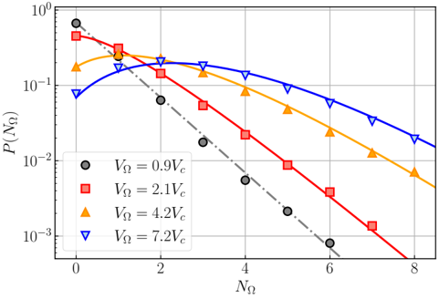
## Line Graph: Probability Distribution of \( N_{\Omega} \) for Different \( V_{\Omega} \) Values ### Overview The image is a scientific line graph plotting the probability \( P(N_{\Omega}) \) against a discrete variable \( N_{\Omega} \) on a semi-logarithmic scale. It displays four distinct data series, each corresponding to a different value of a parameter \( V_{\Omega} \) expressed as a multiple of a critical value \( V_c \). The graph illustrates how the probability distribution changes as \( V_{\Omega} \) increases. ### Components/Axes * **X-Axis (Horizontal):** * **Label:** \( N_{\Omega} \) * **Scale:** Linear, ranging from 0 to 8. Major tick marks are at intervals of 2 (0, 2, 4, 6, 8). * **Y-Axis (Vertical):** * **Label:** \( P(N_{\Omega}) \) * **Scale:** Logarithmic (base 10), ranging from \( 10^{-3} \) to \( 10^{0} \) (0.001 to 1). Major tick marks are at each power of 10. * **Legend:** * **Position:** Top-left corner of the plot area. * **Entries:** 1. **Black circle marker with a dashed black line:** \( V_{\Omega} = 0.9V_c \) 2. **Red square marker with a solid red line:** \( V_{\Omega} = 2.1V_c \) 3. **Orange upward-pointing triangle marker with a solid orange line:** \( V_{\Omega} = 4.2V_c \) 4. **Blue downward-pointing triangle marker with a solid blue line:** \( V_{\Omega} = 7.2V_c \) * **Grid:** A light gray grid is present, aligning with the major ticks on both axes. ### Detailed Analysis The graph shows four probability distributions, each decaying with increasing \( N_{\Omega} \), but at markedly different rates. 1. **Series 1: \( V_{\Omega} = 0.9V_c \) (Black circles, dashed line)** * **Trend:** Steepest exponential decay. The probability drops rapidly by several orders of magnitude as \( N_{\Omega} \) increases. * **Approximate Data Points:** * \( N_{\Omega} = 0 \): \( P \approx 0.7 \) * \( N_{\Omega} = 1 \): \( P \approx 0.25 \) * \( N_{\Omega} = 2 \): \( P \approx 0.07 \) * \( N_{\Omega} = 3 \): \( P \approx 0.02 \) * \( N_{\Omega} = 4 \): \( P \approx 0.005 \) * \( N_{\Omega} = 5 \): \( P \approx 0.0015 \) * \( N_{\Omega} = 6 \): \( P \approx 0.0008 \) (approaching the lower axis limit) 2. **Series 2: \( V_{\Omega} = 2.1V_c \) (Red squares, solid line)** * **Trend:** Steep decay, but less severe than the \( 0.9V_c \) series. * **Approximate Data Points:** * \( N_{\Omega} = 0 \): \( P \approx 0.4 \) * \( N_{\Omega} = 1 \): \( P \approx 0.25 \) * \( N_{\Omega} = 2 \): \( P \approx 0.15 \) * \( N_{\Omega} = 3 \): \( P \approx 0.05 \) * \( N_{\Omega} = 4 \): \( P \approx 0.02 \) * \( N_{\Omega} = 5 \): \( P \approx 0.007 \) * \( N_{\Omega} = 6 \): \( P \approx 0.004 \) * \( N_{\Omega} = 7 \): \( P \approx 0.0012 \) * \( N_{\Omega} = 8 \): \( P \approx 0.0004 \) (approaching the lower axis limit) 3. **Series 3: \( V_{\Omega} = 4.2V_c \) (Orange triangles, solid line)** * **Trend:** Moderate, gradual decay. The distribution is significantly broader. * **Approximate Data Points:** * \( N_{\Omega} = 0 \): \( P \approx 0.18 \) * \( N_{\Omega} = 1 \): \( P \approx 0.22 \) * \( N_{\Omega} = 2 \): \( P \approx 0.18 \) * \( N_{\Omega} = 3 \): \( P \approx 0.15 \) * \( N_{\Omega} = 4 \): \( P \approx 0.08 \) * \( N_{\Omega} = 5 \): \( P \approx 0.04 \) * \( N_{\Omega} = 6 \): \( P \approx 0.02 \) * \( N_{\Omega} = 7 \): \( P \approx 0.01 \) * \( N_{\Omega} = 8 \): \( P \approx 0.006 \) 4. **Series 4: \( V_{\Omega} = 7.2V_c \) (Blue inverted triangles, solid line)** * **Trend:** Slowest decay, resulting in the broadest distribution. Probability remains relatively high across the entire range of \( N_{\Omega} \). * **Approximate Data Points:** * \( N_{\Omega} = 0 \): \( P \approx 0.08 \) * \( N_{\Omega} = 1 \): \( P \approx 0.12 \) * \( N_{\Omega} = 2 \): \( P \approx 0.18 \) * \( N_{\Omega} = 3 \): \( P \approx 0.18 \) * \( N_{\Omega} = 4 \): \( P \approx 0.12 \) * \( N_{\Omega} = 5 \): \( P \approx 0.08 \) * \( N_{\Omega} = 6 \): \( P \approx 0.04 \) * \( N_{\Omega} = 7 \): \( P \approx 0.02 \) * \( N_{\Omega} = 8 \): \( P \approx 0.015 \) ### Key Observations * **Systematic Trend:** As the parameter \( V_{\Omega} \) increases (from \( 0.9V_c \) to \( 7.2V_c \)), the probability distribution \( P(N_{\Omega}) \) becomes progressively broader and decays more slowly with increasing \( N_{\Omega} \). * **Peak Shift:** For the two highest \( V_{\Omega} \) values (4.2V_c and 7.2V_c), the maximum probability does not occur at \( N_{\Omega}=0 \), but at \( N_{\Omega}=1 \) and \( N_{\Omega}=2-3 \), respectively. * **Order-of-Magnitude Differences:** At \( N_{\Omega}=6 \), the probability for \( V_{\Omega}=0.9V_c \) is ~0.0008, while for \( V_{\Omega}=7.2V_c \) it is ~0.04—a difference of approximately 50 times. * **No Outliers:** All data series follow smooth, monotonic (after the initial point for high \( V_{\Omega} \)) trends without anomalous points. ### Interpretation This graph demonstrates a clear physical or statistical relationship where the control parameter \( V_{\Omega} \) (normalized by a critical value \( V_c \)) governs the spread of the distribution of the variable \( N_{\Omega} \). * **Low \( V_{\Omega} \) (Sub-critical, \( 0.9V_c \)):** The system is highly constrained. The probability is overwhelmingly concentrated at the lowest possible value of \( N_{\Omega} \) (0), with a very low likelihood of observing larger values. This suggests a "frozen" or highly ordered state. * **High \( V_{\Omega} \) (Super-critical, \( 7.2V_c \)):** The system is much more "excited" or disordered. The probability is distributed more evenly across a wide range of \( N_{\Omega} \) values, indicating that larger fluctuations or higher states are readily accessible. * **Critical Region:** The transition from a sharply peaked distribution to a broad one occurs as \( V_{\Omega} \) crosses \( V_c \). The series for \( 2.1V_c \) and \( 4.2V_c \) represent intermediate states in this transition. The data suggests \( V_{\Omega} \) acts like a temperature or energy parameter in a statistical system, where increasing it populates higher-energy (larger \( N_{\Omega} \)) states. The precise exponential forms of the decays could be used to extract underlying physical constants or verify a theoretical model.