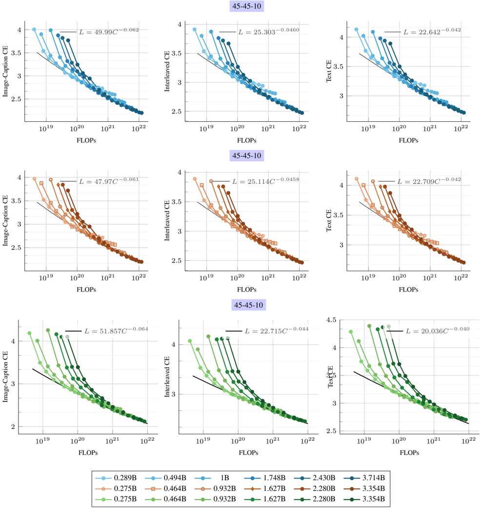
## Line Charts: Scaling Laws for Multimodal Model Performance ### Overview The image displays a 3x3 grid of line charts illustrating the relationship between computational cost (FLOPs) and model performance (Cross-Entropy loss) for multimodal AI models. The charts are organized into three rows, each representing a different model configuration or training run, labeled "45-45-10". Each row uses a distinct color scheme (blue, orange, green) and contains three charts measuring different loss metrics: Image-Caption CE, Interleaved CE, and Text CE. All charts show a clear downward trend, indicating that loss decreases as computational resources increase, following a power-law relationship. ### Components/Axes * **Chart Grid:** 3 rows x 3 columns. * **Row Titles:** Each row is labeled with a purple box containing the text "45-45-10". * **Column Titles (Y-Axis Labels):** * Left Column: "Image-Caption CE" * Middle Column: "Interleaved CE" * Right Column: "Text CE" * **X-Axis:** Labeled "FLOPs" on all charts. The scale is logarithmic, with major tick marks at 10¹⁹, 10²⁰, 10²¹, and 10²². * **Y-Axis:** Represents Cross-Entropy (CE) loss. The scale is linear but the range varies slightly per chart (generally between 2.0 and 4.5). * **Data Series:** Each chart contains multiple lines, each corresponding to a model of a specific size (parameter count). The lines are distinguished by color shade and marker style. * **Legend:** Positioned at the bottom center of the entire figure. It is organized into three rows, corresponding to the three chart rows (blue, orange, green). Each entry shows a colored marker and a model size label. * **Blue Row (Top):** 0.289B, 0.494B, 1B, 1.748B, 2.430B, 3.714B * **Orange Row (Middle):** 0.275B, 0.464B, 0.932B, 1.627B, 2.280B, 3.354B * **Green Row (Bottom):** 0.275B, 0.464B, 0.932B, 1.627B, 2.280B, 3.354B * **Power-Law Fit Equations:** Each chart displays a fitted equation of the form `L = a * C^b`, where `L` is loss and `C` is compute (FLOPs). The specific equations are: * **Top Row (Blue):** * Image-Caption CE: `L = 49.99C^(-0.062)` * Interleaved CE: `L = 25.303C^(-0.0460)` * Text CE: `L = 22.642C^(-0.042)` * **Middle Row (Orange):** * Image-Caption CE: `L = 47.97C^(-0.061)` * Interleaved CE: `L = 25.114C^(-0.0458)` * Text CE: `L = 22.709C^(-0.042)` * **Bottom Row (Green):** * Image-Caption CE: `L = 51.857C^(-0.064)` * Interleaved CE: `L = 22.715C^(-0.044)` * Text CE: `L = 20.036C^(-0.040)` ### Detailed Analysis **Trend Verification:** In every single chart, all data series lines slope downward from left to right. This confirms the universal trend: as FLOPs increase (moving right on the x-axis), the Cross-Entropy loss decreases (moving down on the y-axis). **Component Isolation & Data Extraction:** * **Header Region (Row Labels):** The "45-45-10" label is consistently placed at the top-center of each row of charts. * **Main Chart Region (Per Row):** * **Top Row (Blue Charts):** Models range from 0.289B to 3.714B parameters. For a fixed FLOP count (e.g., 10²⁰), larger models (darker blue) consistently achieve lower loss than smaller models (lighter blue). The power-law exponent `b` is most negative for Image-Caption CE (-0.062), indicating loss improves most rapidly with compute for this metric. * **Middle Row (Orange Charts):** Models range from 0.275B to 3.354B parameters. The scaling behavior is nearly identical to the blue row. The exponents are very similar: Image-Caption CE (-0.061), Interleaved CE (-0.0458), Text CE (-0.042). * **Bottom Row (Green Charts):** Models range from 0.275B to 3.354B parameters. The scaling trends hold. The exponents are slightly different, with Text CE showing the smallest magnitude (-0.040), suggesting its performance improves slightly more slowly with additional compute compared to the other metrics in this run. * **Footer Region (Legend):** The legend is a 3x6 grid. The color and marker for each entry must be matched to the lines in the corresponding row of charts. For example, the darkest blue circle (3.714B) corresponds to the lowest line in the top-left chart. ### Key Observations 1. **Consistent Power-Law Scaling:** All nine charts demonstrate a strong power-law relationship between compute (FLOPs) and loss. The fitted equations have high visual agreement with the data points. 2. **Model Size Advantage:** Within any given chart (fixed metric and training run), larger models (more parameters) are more compute-efficient. They achieve the same loss level at a lower FLOP count, or a lower loss at the same FLOP count, compared to smaller models. 3. **Metric-Specific Scaling Rates:** The exponent `b` in the power-law fit varies by metric. Across all rows, the exponent is largest in magnitude (most negative) for "Image-Caption CE" (~ -0.062), intermediate for "Interleaved CE" (~ -0.045), and smallest for "Text CE" (~ -0.042). This suggests that performance on image-captioning tasks benefits more from additional compute than pure text tasks in these experiments. 4. **Similarity Across Runs:** The three rows (blue, orange, green) show remarkably similar scaling laws, despite likely representing different model initializations or training runs (as indicated by slightly different model size lists and fit parameters). This indicates the observed scaling behavior is robust. ### Interpretation This data provides empirical evidence for **scaling laws in multimodal AI models**. The core finding is that model performance, measured by cross-entropy loss on various tasks, improves predictably as a power-law function of the computational resources (FLOPs) used for training. The "45-45-10" label likely refers to the data mixture ratio used during training (e.g., 45% image-text pairs, 45% interleaved image-text data, 10% text-only data). The three columns then evaluate the model's performance on held-out data from each of these modalities. The key implication is that **increasing compute is a reliable lever for improving multimodal model capabilities**, and the returns follow a diminishing but predictable curve. The fact that larger models are more compute-efficient suggests that for a fixed compute budget, it is better to train a larger model for fewer steps than a smaller model for more steps. The slightly steeper scaling for image-captioning loss might indicate that aligning visual and textual representations is a more compute-intensive process than modeling text alone. This chart would be critical for researchers and engineers planning training runs, as it allows them to forecast the expected performance gain for a given investment in computational resources.