\n
## Line Chart: Principal Curvatures vs. Number of Samples
### Overview
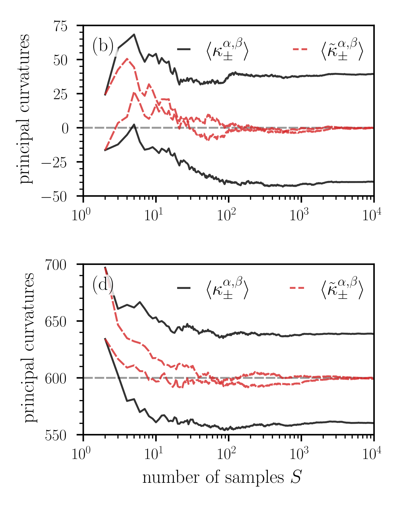
The image contains two vertically stacked line charts, labeled (b) and (d), which plot "principal curvatures" against the "number of samples S" on a logarithmic scale. Each chart compares two different methods or estimators for calculating these curvatures, represented by solid black and dashed red lines. The data shows how the estimated curvature values converge as the sample size increases.
### Components/Axes
**Common Elements:**
* **X-Axis (Both Plots):** Labeled "number of samples S". It uses a logarithmic scale with major tick marks at \(10^0\), \(10^1\), \(10^2\), \(10^3\), and \(10^4\).
* **Y-Axis (Both Plots):** Labeled "principal curvatures". The scale is linear but differs significantly between the two plots.
* **Legend (Both Plots):** Located in the top-right quadrant of each plot area.
* Solid black line (—): Represents the quantity \(\langle \kappa_{\pm}^{\alpha,\beta} \rangle\).
* Dashed red line (--): Represents the quantity \(\langle \tilde{\kappa}_{\pm}^{\alpha,\beta} \rangle\).
* **Reference Lines:** A horizontal dashed gray line is present in both plots, serving as a baseline reference.
**Plot (b) Specifics:**
* **Y-Axis Range:** Approximately -50 to 75.
* **Reference Line:** Positioned at y = 0.
* **Data Series:** Four distinct lines are visible: two solid black and two dashed red. This suggests the plot shows both the positive and negative principal curvature estimates for each method.
**Plot (d) Specifics:**
* **Y-Axis Range:** Approximately 550 to 700.
* **Reference Line:** Positioned at y = 600.
* **Data Series:** Similar to plot (b), there are four lines: two solid black and two dashed red.
### Detailed Analysis
**Plot (b) Analysis:**
* **Trend Verification:**
* **Black Lines (\(\langle \kappa_{\pm}^{\alpha,\beta} \rangle\)):** One line starts near -15 at S=2, rises sharply to a peak near 0 at S≈5, then declines steadily, stabilizing around -40 for S > 100. The other black line starts near 25, rises to a peak near 70 at S≈5, then declines and stabilizes around 40 for S > 100. The two lines diverge from a common region and then stabilize at symmetric values around zero.
* **Red Lines (\(\langle \tilde{\kappa}_{\pm}^{\alpha,\beta} \rangle\)):** Both lines show high volatility for S < 100, oscillating roughly between -10 and 50. For S > 100, they converge and stabilize very close to the y=0 reference line.
* **Key Data Points (Approximate):**
* At S=2: Black lines ≈ -15 and 25; Red lines ≈ -15 and 25.
* At S=5 (Peak for black lines): Upper black ≈ 70, Lower black ≈ 0.
* At S=100: Upper black ≈ 40, Lower black ≈ -40; Red lines ≈ 0.
* At S=10,000: Upper black ≈ 40, Lower black ≈ -40; Red lines ≈ 0.
**Plot (d) Analysis:**
* **Trend Verification:**
* **Black Lines (\(\langle \kappa_{\pm}^{\alpha,\beta} \rangle\)):** One line starts near 635 at S=2, drops sharply to about 560 by S=10, then gradually declines further, stabilizing around 560 for S > 100. The other black line starts near 700, drops to about 660 by S=10, then declines more gradually, stabilizing around 640 for S > 100.
* **Red Lines (\(\langle \tilde{\kappa}_{\pm}^{\alpha,\beta} \rangle\)):** Both lines start near 700 at S=2, drop rapidly, and then fluctuate around the y=600 reference line for S > 10, showing much less variance than the black lines in the mid-range.
* **Key Data Points (Approximate):**
* At S=2: All lines start near 700.
* At S=10: Upper black ≈ 660, Lower black ≈ 560; Red lines ≈ 620 and 610.
* At S=100: Upper black ≈ 640, Lower black ≈ 560; Red lines ≈ 600.
* At S=10,000: Upper black ≈ 640, Lower black ≈ 560; Red lines ≈ 600.
### Key Observations
1. **Convergence with Sample Size:** All estimates show significant volatility for small sample sizes (S < 100) and converge to stable values as S increases towards 10,000.
2. **Method Comparison:** The method represented by the dashed red lines (\(\langle \tilde{\kappa}_{\pm}^{\alpha,\beta} \rangle\)) consistently converges to the reference line (0 in plot b, 600 in plot d). The method represented by solid black lines (\(\langle \kappa_{\pm}^{\alpha,\beta} \rangle\)) converges to values symmetrically offset from this reference.
3. **Scale Difference:** Plot (d) deals with curvature values an order of magnitude larger (550-700) than plot (b) (-50 to 75), suggesting it may represent a different geometric feature or a different scale of analysis.
4. **Initial Transient:** The most dramatic changes in estimated values occur for S between 2 and 100, indicating this is the critical range for sample size in these estimations.
### Interpretation
The charts demonstrate the performance and convergence properties of two different estimators for principal curvatures as a function of sample size.
* **What the data suggests:** The estimator \(\langle \tilde{\kappa}_{\pm}^{\alpha,\beta} \rangle\) (red dashed) appears to be an **unbiased or corrected estimator**, as its mean converges to the theoretical or reference value (0 or 600). The estimator \(\langle \kappa_{\pm}^{\alpha,\beta} \rangle\) (black solid) appears to be a **biased estimator**, converging to values that are symmetrically offset from the reference. The bias is consistent and stable for large S.
* **Relationship between elements:** The two plots likely show the same analysis applied to two different datasets or geometric contexts (e.g., different manifolds or regions of a manifold), given the vastly different curvature scales. The symmetric offset of the black lines around the red convergence line in both plots is a key pattern, suggesting a systematic relationship between the two estimators.
* **Notable patterns:** The initial high volatility for small S is expected in statistical estimation. The fact that the biased estimator (black) shows a clear peak/trough structure at very low S (plot b) before settling into its biased convergence path is notable. The charts effectively argue that using the \(\langle \tilde{\kappa}_{\pm}^{\alpha,\beta} \rangle\) method yields estimates that align with the reference value, while the \(\langle \kappa_{\pm}^{\alpha,\beta} \rangle\) method yields precise but systematically offset results. For applications requiring accuracy relative to the reference, the red-dashed method is superior.