## Line Graphs: Principal Curvatures vs. Number of Samples
### Overview
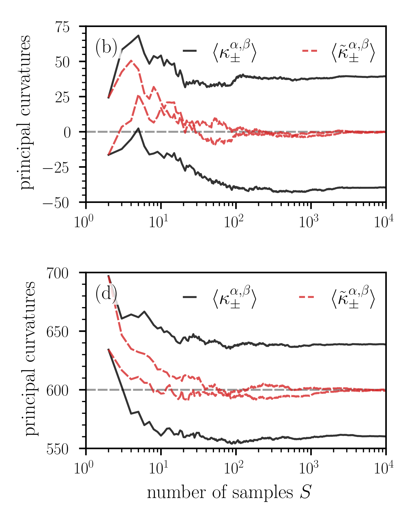
Two line graphs (labeled (b) and (d)) depict the relationship between principal curvatures and the number of samples \( S \) (logarithmic scale). Each graph compares two curvature metrics: a solid black line (\( \langle \kappa_{\alpha,\beta} \rangle \)) and a dashed red line (\( \langle \tilde{\kappa}_{\alpha,\beta} \rangle \)).
### Components/Axes
- **Y-axis**:
- Graph (b): "principal curvatures" ranging from \(-50\) to \(75\).
- Graph (d): "principal curvatures" ranging from \(550\) to \(700\).
- **X-axis**: "number of samples \( S \)" on a logarithmic scale (\(10^0\) to \(10^4\)).
- **Legends**:
- Solid black line: \( \langle \kappa_{\alpha,\beta} \rangle \).
- Dashed red line: \( \langle \tilde{\kappa}_{\alpha,\beta} \rangle \).
- **Placement**: Legends are positioned in the upper-right corner of each graph.
### Detailed Analysis
#### Graph (b)
- **Solid black line (\( \langle \kappa_{\alpha,\beta} \rangle \))**:
- Starts at \( \sim 50 \), peaks near \( 75 \) at \( S = 10^1 \), then declines to \( \sim -25 \) by \( S = 10^4 \).
- Exhibits high variability (oscillations) between \( S = 10^1 \) and \( 10^2 \).
- **Dashed red line (\( \langle \tilde{\kappa}_{\alpha,\beta} \rangle \))**:
- Starts at \( \sim 25 \), peaks near \( 50 \) at \( S = 10^1 \), then declines to \( \sim -25 \) by \( S = 10^4 \).
- Shows sharper oscillations than the black line between \( S = 10^1 \) and \( 10^2 \).
- **Convergence**: Both lines converge near \( -25 \) as \( S \to 10^4 \).
#### Graph (d)
- **Solid black line (\( \langle \kappa_{\alpha,\beta} \rangle \))**:
- Starts at \( \sim 650 \), peaks near \( 700 \) at \( S = 10^1 \), then declines to \( \sim 600 \) by \( S = 10^4 \).
- Smoother trend compared to graph (b).
- **Dashed red line (\( \langle \tilde{\kappa}_{\alpha,\beta} \rangle \))**:
- Starts at \( \sim 600 \), peaks near \( 650 \) at \( S = 10^1 \), then declines to \( \sim 550 \) by \( S = 10^4 \).
- Exhibits minor oscillations but remains relatively stable after \( S = 10^2 \).
- **Convergence**: Both lines converge near \( 550 \) as \( S \to 10^4 \).
### Key Observations
1. **Convergence**: In both graphs, the two curvature metrics (\( \langle \kappa_{\alpha,\beta} \rangle \) and \( \langle \tilde{\kappa}_{\alpha,\beta} \rangle \)) converge as \( S \) increases, suggesting reduced divergence with larger sample sizes.
2. **Initial Peaks**: Both metrics exhibit initial peaks at \( S = 10^1 \), followed by declines.
3. **Amplitude Differences**:
- Graph (b): Curvatures span a wider range (\(-50\) to \(75\)) compared to graph (d) (\(550\) to \(700\)).
- Graph (d): Curvatures remain positive throughout, while graph (b) includes negative values.
### Interpretation
The data suggests that principal curvature estimates stabilize as the number of samples grows. The convergence of \( \langle \kappa_{\alpha,\beta} \rangle \) and \( \langle \tilde{\kappa}_{\alpha,\beta} \rangle \) implies that both metrics agree on curvature values at large \( S \), potentially indicating robustness in the estimation process. The initial variability (especially in graph (b)) may reflect noise or sensitivity to small sample sizes. The logarithmic x-axis emphasizes the impact of exponential sample growth on curvature trends.
**Note**: No textual content in other languages is present. All values are approximate, with uncertainty arising from visual estimation of the plotted lines.