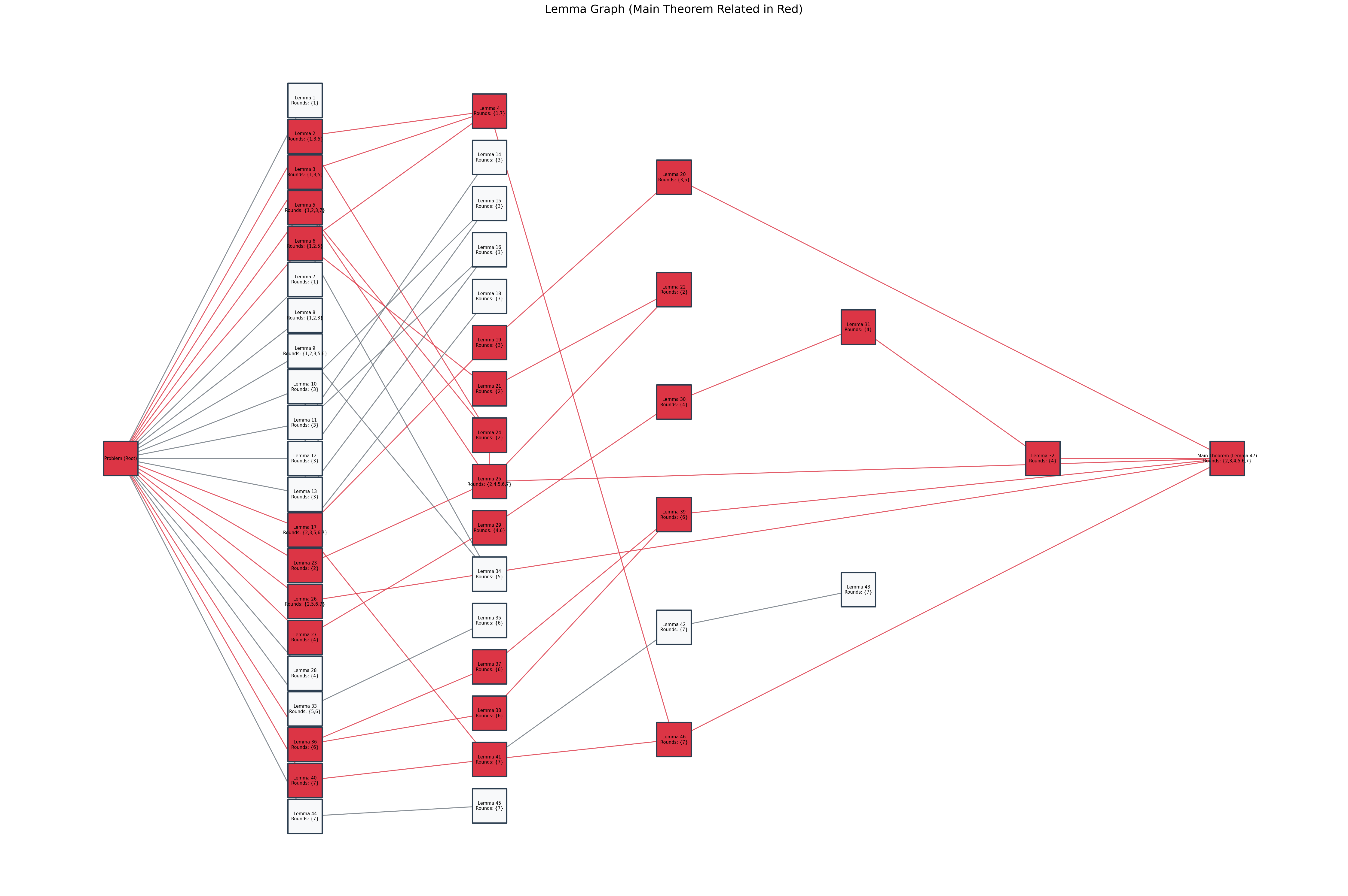
## Diagram: Lemma Graph ### Overview The image is a directed graph representing the relationships between different lemmas and a main theorem. The graph consists of nodes labeled as "Lemma [Number]" or "Problem (Root)" and "Main Theorem (Lemma 47)", with edges connecting these nodes. The nodes are colored either red or gray, with red nodes indicating a direct relationship to the main theorem. Each node also includes information about the "Rounds" associated with it, represented as a set of numbers. ### Components/Axes * **Nodes:** Represented by rectangles, labeled with "Lemma [Number]" or "Problem (Root)" and "Main Theorem (Lemma 47)". Each node also contains "Rounds: {numbers}". * **Edges:** Represented by lines connecting the nodes, indicating a dependency or relationship. Red lines indicate a direct relationship to the Main Theorem. * **Colors:** Red nodes and edges indicate a direct relationship to the Main Theorem. Gray nodes and edges indicate an indirect relationship. * **Title:** "Lemma Graph (Main Theorem Related in Red)" is located at the top of the image. ### Detailed Analysis Here's a breakdown of the nodes and their connections, along with the "Rounds" information: * **Problem (Root):** Located on the left side of the diagram. It is the starting point of the graph. It connects to all the nodes in the second column. * **Lemma 1:** Rounds: {1}. Located in the top-left of the second column. Red node. * **Lemma 2:** Rounds: {1,3,5}. Located in the second position of the second column. Red node. * **Lemma 3:** Rounds: {1,3,5}. Located in the third position of the second column. Red node. * **Lemma 5:** Rounds: {1,2,3,7}. Located in the fourth position of the second column. Red node. * **Lemma 6:** Rounds: {1,2,5}. Located in the fifth position of the second column. Red node. * **Lemma 7:** Rounds: {1}. Located in the sixth position of the second column. Red node. * **Lemma 8:** Rounds: {1,2,3}. Located in the seventh position of the second column. Gray node. * **Lemma 9:** Rounds: {1,2,3,5,6}. Located in the eighth position of the second column. Red node. * **Lemma 10:** Rounds: {3}. Located in the ninth position of the second column. Red node. * **Lemma 11:** Rounds: {3}. Located in the tenth position of the second column. Gray node. * **Lemma 12:** Rounds: {3}. Located in the eleventh position of the second column. Gray node. * **Lemma 13:** Rounds: {3}. Located in the twelfth position of the second column. Gray node. * **Lemma 17:** Rounds: {2,3,5,6,7}. Located in the thirteenth position of the second column. Red node. * **Lemma 23:** Rounds: {2}. Located in the fourteenth position of the second column. Red node. * **Lemma 26:** Rounds: {2,5,6,7}. Located in the fifteenth position of the second column. Red node. * **Lemma 27:** Rounds: {4}. Located in the sixteenth position of the second column. Red node. * **Lemma 28:** Rounds: {4}. Located in the seventeenth position of the second column. Red node. * **Lemma 33:** Rounds: {5,6}. Located in the eighteenth position of the second column. Red node. * **Lemma 36:** Rounds: {6}. Located in the nineteenth position of the second column. Red node. * **Lemma 40:** Rounds: {7}. Located in the twentieth position of the second column. Red node. * **Lemma 44:** Rounds: {7}. Located in the twenty-first position of the second column. Red node. * **Lemma 4:** Rounds: {1,7}. Located in the top-left of the third column. Red node. * **Lemma 14:** Rounds: {3}. Located in the second position of the third column. Red node. * **Lemma 15:** Rounds: {3}. Located in the third position of the third column. Gray node. * **Lemma 16:** Rounds: {3}. Located in the fourth position of the third column. Gray node. * **Lemma 18:** Rounds: {3}. Located in the fifth position of the third column. Gray node. * **Lemma 19:** Rounds: {3}. Located in the sixth position of the third column. Red node. * **Lemma 21:** Rounds: {2}. Located in the seventh position of the third column. Red node. * **Lemma 24:** Rounds: {2}. Located in the eighth position of the third column. Red node. * **Lemma 25:** Rounds: {2,4,5,6,7}. Located in the ninth position of the third column. Red node. * **Lemma 29:** Rounds: {4,6}. Located in the tenth position of the third column. Red node. * **Lemma 34:** Rounds: {5}. Located in the eleventh position of the third column. Gray node. * **Lemma 35:** Rounds: {6}. Located in the twelfth position of the third column. Red node. * **Lemma 37:** Rounds: {6}. Located in the thirteenth position of the third column. Red node. * **Lemma 38:** Rounds: {6}. Located in the fourteenth position of the third column. Gray node. * **Lemma 41:** Rounds: {7}. Located in the fifteenth position of the third column. Red node. * **Lemma 45:** Rounds: {7}. Located in the sixteenth position of the third column. Red node. * **Lemma 20:** Rounds: {3,5}. Located in the top-left of the fourth column. Red node. * **Lemma 22:** Rounds: {2}. Located in the second position of the fourth column. Red node. * **Lemma 30:** Rounds: {4}. Located in the third position of the fourth column. Red node. * **Lemma 31:** Rounds: {4}. Located in the fourth position of the fourth column. Red node. * **Lemma 39:** Rounds: {6}. Located in the fifth position of the fourth column. Red node. * **Lemma 42:** Rounds: {7}. Located in the sixth position of the fourth column. Red node. * **Lemma 43:** Rounds: {7}. Located in the seventh position of the fourth column. Gray node. * **Lemma 46:** Rounds: {7}. Located in the eighth position of the fourth column. Red node. * **Main Theorem (Lemma 47):** Rounds: {2,3,4,5,6,7}. Located on the right side of the diagram. Red node. ### Key Observations * The "Problem (Root)" node connects to all nodes in the second column. * Red nodes indicate a direct relationship to the "Main Theorem (Lemma 47)". * Gray nodes indicate an indirect relationship to the "Main Theorem (Lemma 47)". * The "Rounds" information varies for each lemma. * The "Main Theorem (Lemma 47)" node is the destination of many red edges. ### Interpretation The diagram illustrates the dependencies between different lemmas and how they contribute to proving the "Main Theorem (Lemma 47)". The red nodes and edges highlight the lemmas that are directly involved in proving the main theorem, while the gray nodes represent lemmas that are indirectly related or serve as supporting lemmas. The "Rounds" information likely refers to specific rounds or iterations in a proof or algorithm where the lemma is relevant. The graph structure provides a visual representation of the logical flow and dependencies within the proof. The "Problem (Root)" serves as the initial condition or starting point for the chain of reasoning leading to the main theorem.

\n ## Diagram: Lemma Graph (Main Theorem Related in Red) ### Overview The image presents a diagram representing a lemma graph, likely related to a mathematical theorem. The graph consists of rectangular nodes connected by lines, indicating relationships between lemmas. The main theorem is visually highlighted in red. The diagram appears to illustrate dependencies and connections between various lemmas contributing to the proof of the main theorem. ### Components/Axes The diagram consists of: * **Nodes:** Rectangular boxes labeled "Lemma [Number]" and "Results [Number]". * **Connections:** Lines connecting the nodes, representing dependencies or relationships. * **Color Coding:** Red color is used to highlight the main theorem. * **Title:** "Lemma Graph (Main Theorem Related in Red)" positioned at the top-center. * **Central Node:** A node labeled "Results (1.2.4.1)" is positioned near the center of the diagram. * **Starting Node:** A node labeled "Problem" is positioned on the left side of the diagram. * **Ending Nodes:** Several nodes labeled "Lemma [Number]" are positioned on the right side of the diagram. ### Detailed Analysis or Content Details The diagram contains a large number of lemmas and results. Here's a breakdown of the visible nodes and their connections: * **Problem Node (Left):** This is the starting point of the graph. * **Central Results Node:** "Results (1.2.4.1)" is heavily connected to many lemmas. * **Main Theorem (Right):** Highlighted in red, it appears to be a final result derived from the lemmas. * **Lemma Nodes (Left):** A cluster of lemmas connected to the "Problem" node. These include: * Lemma 1 (Results: 1) * Lemma 2 (Results: 1) * Lemma 3 (Results: 1) * Lemma 4 (Results: 1) * Lemma 5 (Results: 1) * Lemma 6 (Results: 1) * Lemma 7 (Results: 1) * Lemma 8 (Results: 1) * Lemma 9 (Results: 1) * Lemma 10 (Results: 1) * **Lemma Nodes (Center-Left):** Another cluster of lemmas connected to the central "Results (1.2.4.1)" node. These include: * Lemma 11 (Results: 1) * Lemma 12 (Results: 1) * Lemma 13 (Results: 1) * Lemma 14 (Results: 1) * Lemma 15 (Results: 1) * Lemma 16 (Results: 1) * Lemma 17 (Results: 1) * Lemma 18 (Results: 1) * **Lemma Nodes (Center-Right):** A cluster of lemmas connected to the central "Results (1.2.4.1)" node. These include: * Lemma 19 (Results: 1) * Lemma 20 (Results: 1) * Lemma 21 (Results: 1) * Lemma 22 (Results: 1) * Lemma 23 (Results: 1) * Lemma 24 (Results: 1) * **Lemma Nodes (Right):** A cluster of lemmas connected to the main theorem. These include: * Lemma 25 (Results: 1) * Lemma 26 (Results: 1) * Lemma 27 (Results: 1) * Lemma 28 (Results: 1) * Lemma 29 (Results: 1) The connections are mostly one-way, indicating a direction of dependency. The "Problem" node has many outgoing connections, while the main theorem has several incoming connections. The central "Results (1.2.4.1)" node acts as a hub, connecting many lemmas. ### Key Observations * The diagram is highly interconnected, suggesting a complex relationship between the lemmas. * The central "Results (1.2.4.1)" node is a critical component, linking many lemmas together. * The main theorem is dependent on a large number of lemmas. * The diagram does not provide any quantitative data, only qualitative relationships. * The "Results [Number]" notation suggests that each lemma leads to a specific result. ### Interpretation The diagram visually represents the logical structure of a mathematical proof. The "Problem" node represents the initial statement or question, and the main theorem represents the final conclusion. The lemmas are intermediate steps in the proof, and the lines indicate the dependencies between them. The diagram suggests that the proof is built upon a foundation of interconnected lemmas, with the central "Results (1.2.4.1)" node playing a crucial role in connecting these lemmas to the final theorem. The red highlighting of the main theorem emphasizes its importance as the ultimate goal of the proof. The diagram is a high-level overview of the proof structure and does not provide details about the specific content of each lemma. It is a visual aid for understanding the overall flow of the proof and the relationships between its components. The diagram is a form of knowledge representation, showing how different pieces of mathematical knowledge are connected to achieve a specific result.

\n ## Lemma Dependency Graph: Main Theorem Proof Structure ### Overview This image is a directed graph visualizing the logical dependencies between a set of lemmas (numbered 1 through 47) and a central "Problem (Root)" leading to a "Main Theorem (Lemma 47)". The graph is titled **"Lemma Graph (Main Theorem Related in Red)"**. Nodes represent lemmas or the problem/theorem, and directed edges (arrows) indicate that one lemma is used to prove another. Nodes are colored either red or white; red nodes are explicitly related to the proof of the Main Theorem. The layout progresses from left (root problem) to right (final theorem), with intermediate lemmas arranged in vertical columns. ### Components/Axes * **Title:** "Lemma Graph (Main Theorem Related in Red)" (top center). * **Node Types:** * **Root Node:** A single red square on the far left labeled "Problem (Root)". * **Lemma Nodes:** 46 squares labeled "Lemma [Number]" with a secondary line "Rounds: [List of numbers]". * **Terminal Node:** A single red square on the far right labeled "Main Theorem (Lemma 47)" with "Rounds: [2,3,4,5,6,7]". * **Node Attributes:** * **Color:** Red or White. Per the title, red nodes are "Main Theorem Related". * **Text:** Each node contains a label (e.g., "Lemma 1") and a "Rounds" list (e.g., "Rounds: (1)"). * **Edges:** Directed arrows connecting nodes. They are colored either **red** or **gray**. Red edges appear to connect nodes within the "Main Theorem Related" (red) set or from a red node to another node critical to the theorem's path. * **Spatial Layout:** Nodes are arranged in approximately 7 vertical columns from left to right. The "Problem (Root)" is in column 1. The "Main Theorem" is in the final column on the right. Intermediate lemmas are distributed across columns 2 through 6. ### Detailed Analysis **Node Inventory (Listed by approximate column, top to bottom):** * **Column 1 (Root):** * `Problem (Root)` [Red] * **Column 2:** * `Lemma 1` [White], Rounds: (1) * `Lemma 2` [Red], Rounds: (1,3,5) * `Lemma 3` [Red], Rounds: (1,3,5) * `Lemma 5` [Red], Rounds: (1,2,3,4) * `Lemma 6` [Red], Rounds: (1,2,5) * `Lemma 7` [White], Rounds: (1) * `Lemma 8` [White], Rounds: (1,2,3) * `Lemma 9` [White], Rounds: (1,2,3,5,6) * `Lemma 10` [White], Rounds: (3) * `Lemma 11` [White], Rounds: (3) * `Lemma 12` [White], Rounds: (3) * `Lemma 13` [White], Rounds: (3) * `Lemma 17` [Red], Rounds: (2,3,5,6,7) * `Lemma 23` [Red], Rounds: (2) * `Lemma 26` [Red], Rounds: (2,5,6,7) * `Lemma 27` [Red], Rounds: (4) * `Lemma 28` [White], Rounds: (4) * `Lemma 33` [White], Rounds: (5,6) * `Lemma 36` [Red], Rounds: (6) * `Lemma 40` [Red], Rounds: (7) * `Lemma 44` [White], Rounds: (7) * **Column 3:** * `Lemma 4` [Red], Rounds: (1,7) * `Lemma 14` [White], Rounds: (3) * `Lemma 15` [White], Rounds: (3) * `Lemma 16` [White], Rounds: (3) * `Lemma 18` [White], Rounds: (3) * `Lemma 19` [Red], Rounds: (3) * `Lemma 21` [Red], Rounds: (2) * `Lemma 24` [Red], Rounds: (2) * `Lemma 25` [Red], Rounds: (2,4,5,6,7) * `Lemma 29` [Red], Rounds: (4,6) * `Lemma 34` [White], Rounds: (5) * `Lemma 35` [White], Rounds: (6) * `Lemma 37` [Red], Rounds: (6) * `Lemma 38` [Red], Rounds: (6) * `Lemma 41` [Red], Rounds: (7) * `Lemma 45` [White], Rounds: (7) * **Column 4:** * `Lemma 20` [Red], Rounds: (3,5) * `Lemma 22` [Red], Rounds: (2) * `Lemma 30` [Red], Rounds: (4) * `Lemma 39` [Red], Rounds: (6) * `Lemma 42` [White], Rounds: (7) * `Lemma 46` [Red], Rounds: (7) * **Column 5:** * `Lemma 31` [Red], Rounds: (4) * `Lemma 43` [White], Rounds: (7) * **Column 6:** * `Lemma 32` [Red], Rounds: (4) * **Column 7 (Terminal):** * `Main Theorem (Lemma 47)` [Red], Rounds: (2,3,4,5,6,7) **Connection Analysis (Key Paths):** The graph shows a dense network of dependencies. The "Problem (Root)" has outgoing edges to nearly all lemmas in Column 2. The "Main Theorem" has incoming edges from several red nodes in the preceding columns, most directly from `Lemma 32`, `Lemma 25`, `Lemma 29`, `Lemma 39`, and `Lemma 46`. The red edges highlight a core network of lemmas (e.g., 2, 3, 5, 6, 17, 19, 21, 24, 25, 29, 30, 31, 32, 36, 37, 38, 39, 40, 41, 46) that are all interconnected and ultimately feed into the Main Theorem. ### Key Observations 1. **Color Coding:** There is a clear distinction between red nodes (theorem-related) and white nodes. All nodes in the final two columns (except `Lemma 43`) are red, indicating they are part of the final proof chain. 2. **Rounds Metadata:** The "Rounds" list for each lemma likely indicates in which proof rounds or stages that lemma is utilized. The Main Theorem itself is used in rounds 2 through 7. 3. **Graph Density:** The dependency graph is highly interconnected, especially among the red nodes, suggesting a complex, non-linear proof structure where many lemmas support each other. 4. **Spatial Flow:** The left-to-right layout effectively visualizes the progression from the initial problem, through layers of intermediate results (lemmas), to the final theorem. The convergence of edges onto the Main Theorem node is visually prominent. ### Interpretation This graph is a **proof dependency map** for a complex mathematical or theoretical computer science result. It answers the question: "What foundational statements (lemmas) are needed, and in what logical order, to prove the Main Theorem?" * **What it demonstrates:** The proof is not a simple linear chain. It is a web of interdependent results. The red nodes and edges trace the **critical path** or the essential backbone of lemmas directly contributing to the final theorem. White nodes represent supporting lemmas that are used in the proof but are not themselves directly part of the final theorem's statement or immediate logical ancestry. * **Relationships:** An edge from Lemma A to Lemma B means "Lemma A is used in the proof of Lemma B." The "Rounds" data adds a temporal or procedural dimension, showing when each piece of the argument is deployed across multiple stages of the overall proof. * **Notable Patterns:** The concentration of red nodes and edges in the right half of the graph shows how the proof consolidates as it approaches the conclusion. The presence of red nodes early on (e.g., Lemmas 2, 3, 5, 6) indicates that some fundamental components of the final theorem are established very early in the logical structure. The graph allows a researcher to quickly identify which lemmas are most central (high in-degree/out-degree red nodes) and to understand the proof's architecture at a glance.

## Directed Graph: Lemma Graph (Main Theorem Related in Red) ### Overview The image depicts a directed graph representing logical dependencies between lemmas and axioms, with the "Main Theorem" (Lemma 47) as the central node. Nodes are labeled with "Lemma X" (e.g., Lemma 4, Lemma 21) and "Axiom Y" (e.g., Axiom 1, Axiom 2). Red edges and nodes highlight the main theorem-related lemmas, while gray edges and nodes represent auxiliary or intermediate steps. The graph is structured in a hierarchical, tree-like format with the "Problem State" as the root and the "Main Theorem" as the terminal node. ### Components/Axes - **Nodes**: - **Problem State**: Root node (leftmost column). - **Lemmas**: Labeled as "Lemma X" (e.g., Lemma 1, Lemma 4, Lemma 21, Lemma 47). - **Axioms**: Labeled as "Axiom Y" (e.g., Axiom 1, Axiom 2). - **Main Theorem**: "Main Theorem (Lemma 47)" (rightmost node). - **Edges**: - **Red edges**: Connect nodes related to the main theorem. - **Gray edges**: Connect auxiliary or intermediate steps. - **Legend**: - Red color indicates "Main Theorem Related" (applies to nodes and edges). - Gray color indicates non-main theorem-related elements. ### Detailed Analysis - **Node Labels**: - **Lemmas**: - Lemma 1 (Axiom 1) - Lemma 4 (Axiom 1) - Lemma 14 (Axiom 3) - Lemma 21 (Axiom 2) - Lemma 29 (Axiom 2) - Lemma 47 (Main Theorem) - **Axioms**: - Axiom 1 (appears in Lemma 1, Lemma 4) - Axiom 2 (appears in Lemma 21, Lemma 29) - Axiom 3 (appears in Lemma 14) - **Main Theorem**: Lemma 47 (connected to Lemma 21, Lemma 29, Lemma 43, Lemma 46). - **Edge Connections**: - The "Problem State" connects to Lemma 1, Lemma 4, and Lemma 14. - Lemma 4 connects to Lemma 14, Lemma 21, and Lemma 29. - Lemma 21 connects to Lemma 29, Lemma 43, and Lemma 46. - Lemma 29 connects to Lemma 43, Lemma 46, and Lemma 47. - Lemma 43 connects to Lemma 46 and Lemma 47. - Lemma 46 connects to Lemma 47. - **Color Coding**: - Red nodes/edges: Lemma 4, Lemma 21, Lemma 29, Lemma 47, and their connecting edges. - Gray nodes/edges: All other nodes and edges. ### Key Observations 1. **Central Role of Lemma 47**: The Main Theorem (Lemma 47) is the terminal node, connected to multiple lemmas (21, 29, 43, 46), indicating it synthesizes prior results. 2. **Hierarchical Structure**: The graph progresses from the Problem State through intermediate lemmas (e.g., Lemma 1, Lemma 4) to the Main Theorem. 3. **Redundancy in Axioms**: Axiom 1 is used in Lemma 1 and Lemma 4, while Axiom 2 is used in Lemma 21 and Lemma 29. 4. **Critical Pathways**: Red edges form a "main theorem pathway" from Lemma 4 → Lemma 21 → Lemma 29 → Lemma 47. ### Interpretation The graph illustrates a logical framework where the Main Theorem (Lemma 47) is derived through a sequence of lemmas and axioms. The red nodes and edges emphasize the critical steps required to reach the theorem, suggesting a dependency chain. The use of Axiom 1 and Axiom 2 in multiple lemmas indicates foundational assumptions. The hierarchical layout implies a structured proof, with the Problem State as the starting point and the Main Theorem as the culmination. The absence of gray nodes in the main pathway highlights the focus on the theorem's derivation. This structure could represent a formal proof system or a dependency graph in a mathematical or computational context.