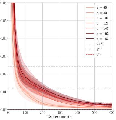
\n ## Line Chart: Convergence of Loss with Gradient Updates ### Overview The image presents a line chart illustrating the convergence of a loss function with respect to the number of gradient updates. Multiple lines represent different values of a parameter 'd', and the chart includes horizontal lines representing theoretical bounds on the loss. The chart appears to demonstrate how the loss decreases as gradient updates are applied, and how this convergence is affected by the value of 'd'. ### Components/Axes * **X-axis:** "Gradient updates", ranging from 0 to approximately 600. * **Y-axis:** Loss value, ranging from 0 to approximately 0.06. * **Legend:** Located in the top-right corner, listing the following lines: * d = 60 (lightest red) * d = 80 (slightly darker red) * d = 100 (medium red) * d = 120 (darker red) * d = 140 (even darker red) * d = 160 (very dark red) * d = 180 (darkest red) * 2 * ε^uni (black dashed line) * ε^uni (black dotted line) * ε^opt (red dashed-dotted line) ### Detailed Analysis The chart displays several lines representing the loss function's value as gradient updates increase. * **d = 60:** Starts at approximately 0.058 and rapidly decreases, leveling off around a loss value of approximately 0.008 at 600 gradient updates. * **d = 80:** Starts at approximately 0.055 and decreases more slowly than d=60, leveling off around a loss value of approximately 0.009 at 600 gradient updates. * **d = 100:** Starts at approximately 0.052 and decreases at a rate between d=60 and d=80, leveling off around a loss value of approximately 0.0095 at 600 gradient updates. * **d = 120:** Starts at approximately 0.049 and decreases at a rate similar to d=100, leveling off around a loss value of approximately 0.0095 at 600 gradient updates. * **d = 140:** Starts at approximately 0.046 and decreases at a rate similar to d=120, leveling off around a loss value of approximately 0.009 at 600 gradient updates. * **d = 160:** Starts at approximately 0.043 and decreases at a rate similar to d=140, leveling off around a loss value of approximately 0.0085 at 600 gradient updates. * **d = 180:** Starts at approximately 0.040 and decreases at a rate similar to d=160, leveling off around a loss value of approximately 0.008 at 600 gradient updates. The horizontal lines represent theoretical bounds: * **2 * ε^uni:** A black dashed line at approximately 0.012. * **ε^uni:** A black dotted line at approximately 0.006. * **ε^opt:** A red dashed-dotted line at approximately 0.004. All lines for different 'd' values converge towards a similar loss value as the number of gradient updates increases, and all lines appear to approach the ε^opt bound. ### Key Observations * The loss decreases rapidly initially for all values of 'd', then the rate of decrease slows down. * Larger values of 'd' (e.g., 180) seem to converge slightly faster than smaller values (e.g., 60), but the difference is minimal. * All lines converge below the 2 * ε^uni bound. * The lines approach, but do not necessarily reach, the ε^opt bound within the observed range of gradient updates. ### Interpretation The chart demonstrates the convergence behavior of a loss function during optimization using gradient updates. The parameter 'd' likely represents a dimensionality or complexity factor within the optimization problem. The convergence is shown to be relatively stable across different values of 'd', suggesting that the optimization process is not overly sensitive to this parameter within the tested range. The horizontal lines (ε^uni and ε^opt) represent theoretical limits on the achievable loss, potentially based on uniform or optimal convergence rates. The fact that the loss values approach these bounds indicates that the optimization process is functioning as expected. The slight differences in convergence rates for different 'd' values suggest that increasing 'd' may offer a marginal improvement in convergence speed, but the benefit is likely limited. The chart provides evidence that the optimization algorithm is effectively reducing the loss function, and that the results are consistent with theoretical expectations.