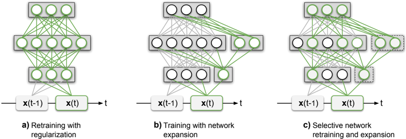
## Diagram: Neural Network Training Strategies ### Overview The image displays three schematic diagrams of artificial neural network architectures, each illustrating a different strategy for training or modifying a network over time. The diagrams are arranged horizontally and labeled a), b), and c). Each diagram consists of a network graph (nodes and connections) positioned above a simple timeline. ### Components/Axes **Common Elements in All Diagrams:** * **Network Graph:** Each diagram shows a feedforward neural network with four layers of nodes (circles). From bottom to top: an input layer (3 nodes), two hidden layers (5 nodes and 3 nodes, respectively), and an output layer (3 nodes). Nodes are grouped within gray rectangular boxes representing layers. * **Connections:** Lines between nodes represent synaptic weights. The color of these lines (green or gray) indicates their training status. * **Timeline:** Located at the bottom of each diagram. It consists of three labeled boxes connected by arrows: * `x(t-1)`: Represents the network state or input at the previous time step. * `x(t)`: Represents the network state or input at the current time step. * `t`: Represents the progression of time. * An arrow points from `x(t-1)` to `x(t)`, and another from `x(t)` to `t`. **Diagram-Specific Labels and Features:** * **a) Retraining with regularization:** * **Label:** "a) Retraining with regularization" (centered below the timeline). * **Network State:** All connection lines between all layers are solid green. This indicates that all weights in the entire network are active and subject to update during the retraining process. * **b) Training with network expansion:** * **Label:** "b) Training with network expansion" (centered below the timeline). * **Network State:** The original network structure from diagram a) is present, but most of its connection lines are now gray, indicating they are frozen or not being updated. * **Expansion:** New components are added, highlighted with dashed gray borders: * A new, separate layer of 2 nodes appears to the right of the original top hidden layer. * A new, single node appears to the right of the original output layer. * **Connections:** New green connection lines are drawn from the original input and hidden layers to these new nodes/layers. The new nodes also have green connections among themselves. This shows the network's capacity is being increased by adding new, trainable modules. * **c) Selective network retraining and expansion:** * **Label:** "c) Selective network retraining and expansion" (centered below the timeline). * **Network State:** This diagram shows a hybrid approach. * **Selective Retraining:** Some original connections remain green (e.g., from the input layer to the first hidden layer, and within the top hidden layer), indicating they are being retrained. Other original connections are gray (frozen). * **Selective Expansion:** Similar to diagram b), new nodes with dashed borders are added (a 2-node layer and a 1-node layer). New green connections are established to and from these new components. * **Key Difference:** Unlike b), not all original connections are frozen. The strategy involves both updating a subset of existing weights and adding new capacity. ### Detailed Analysis The diagrams visually contrast three paradigms for adapting a neural network: 1. **Full Retraining (a):** The entire network is plastic. All parameters (`green lines`) are adjusted during training at time `t`, starting from the state at `t-1`. The "regularization" in the label implies a technique to prevent overfitting during this full update. 2. **Expansion (b):** The existing network (`gray lines`) is frozen, preserving learned knowledge. New capacity (`new nodes with dashed borders` and `new green connections`) is added and trained exclusively. This is a form of continual learning aimed at acquiring new skills without catastrophic forgetting. 3. **Hybrid Selective Approach (c):** This is the most nuanced strategy. It combines: * **Selective Retraining:** A subset of the original network's connections (`green lines within the original structure`) is allowed to update. * **Selective Expansion:** New capacity is added (`dashed-border nodes`) and trained. This approach balances plasticity (updating old knowledge and adding new) with stability (freezing some old knowledge). ### Key Observations * **Color Coding is Critical:** Green consistently signifies "active/trainable," while gray signifies "frozen/inactive." This is the primary visual cue for understanding each strategy. * **Spatial Grounding of Expansion:** In diagrams b) and c), the new components are consistently placed to the **right** of the original network layers they connect to, creating a clear visual distinction between "old" and "new." * **Progressive Complexity:** The diagrams show a progression from a monolithic update (a) to a modular, additive approach (b), culminating in a fine-grained, selective approach (c). * **Temporal Flow:** The timeline (`x(t-1) -> x(t) -> t`) at the bottom of each diagram anchors the process in time, emphasizing that these are strategies for sequential learning or adaptation. ### Interpretation These diagrams illustrate core concepts in **continual learning** or **lifelong learning** for neural networks. The central challenge is learning new tasks over time without forgetting previously learned ones (catastrophic forgetting). * **Diagram a)** represents the naive approach: retrain the whole model on new data. This is simple but often leads to forgetting old knowledge. * **Diagram b)** represents a **fixed feature extractor** or **progressive neural network** approach. By freezing the old network and adding new, separate modules, it guarantees no forgetting but can become inefficient as the network grows. * **Diagram c)** represents more advanced, **parameter-isolation** or **selective synthesis** methods. These algorithms aim to identify which specific parameters (weights) in the old network are important for old tasks and should be frozen, while allowing less critical ones to be updated or repurposed for new tasks, alongside adding new capacity. This seeks an optimal balance between stability (remembering) and plasticity (learning). The visual metaphor effectively communicates that intelligent adaptation isn't just about adding more, but about strategically deciding *what* to keep, *what* to change, and *what* to add. The progression from a) to c) mirrors the evolution of research in this field toward more nuanced and efficient solutions.