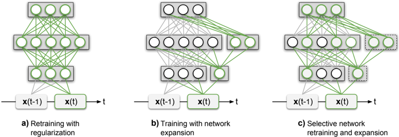
## Diagram: Neural Network Training Methodologies
### Overview
The image presents three comparative diagrams (a, b, c) illustrating different neural network training strategies. Each diagram visualizes the flow of data through layers of nodes, with connections represented by green lines. The diagrams emphasize architectural differences in network expansion, regularization, and selective retraining.
### Components/Axes
- **Labels**:
- **a)** Retraining with regularization
- **b)** Training with network expansion
- **c)** Selective network retraining and expansion
- **Nodes**:
- Input nodes: `x(t-1)` (left) and `x(t)` (center), both highlighted in green.
- Output node: `t` (right).
- Hidden layers: Multiple layers of circular nodes (white with green borders) arranged vertically.
- **Connections**:
- Green lines represent weighted connections between nodes.
- Dashed lines in diagram c) indicate optional or conditional connections.
### Detailed Analysis
1. **Diagram a) (Retraining with regularization)**:
- Dense, fully connected layers with no additional nodes.
- All nodes in hidden layers are interconnected, suggesting a focus on optimizing existing parameters.
2. **Diagram b) (Training with network expansion)**:
- Adds a new layer of nodes (rightmost layer) compared to diagram a).
- Connections extend to the new layer, indicating increased capacity for learning complex patterns.
3. **Diagram c) (Selective network retraining and expansion)**:
- Combines retraining (dense connections in existing layers) with targeted expansion (dashed lines to a single new node).
- Highlights selective activation of nodes, implying efficiency improvements over full expansion.
### Key Observations
- **Architectural Progression**:
- Diagram a) represents the baseline (no expansion).
- Diagram b) introduces full network expansion.
- Diagram c) optimizes expansion by adding only critical nodes.
- **Connection Density**:
- Diagram a) has the highest connection density (fully connected layers).
- Diagram c) reduces density via selective connections, balancing complexity and efficiency.
### Interpretation
The diagrams demonstrate a trade-off between model complexity and efficiency:
- **Regularization (a)** prioritizes stability by limiting overfitting but restricts learning capacity.
- **Full expansion (b)** increases capacity at the cost of computational overhead.
- **Selective expansion (c)** optimizes both by expanding only where necessary, suggesting a middle ground for adaptive learning.
This progression aligns with modern neural network design principles, where efficiency and adaptability are critical for real-time applications. The selective approach in (c) may reflect advancements in dynamic network architectures, such as sparse connectivity or modular learning.