## Diagram: Neural Network Architecture with LBM and Processing Nodes
### Overview
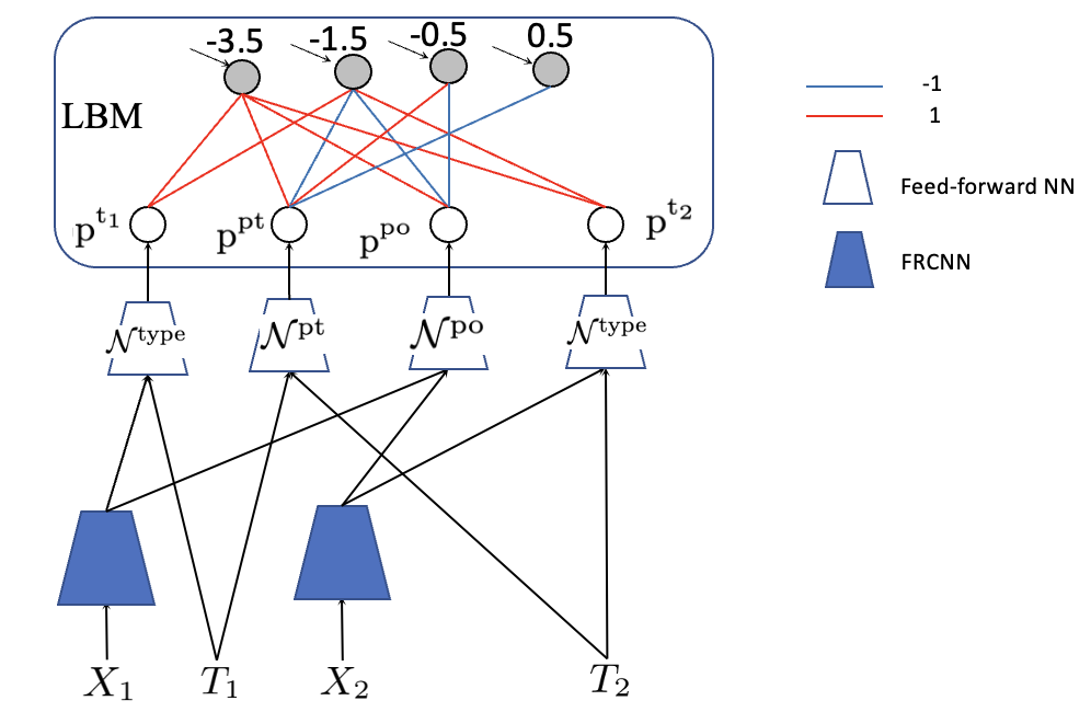
The diagram illustrates a computational architecture combining a Local Binary Model (LBM) with feed-forward and FRCNN (Feed-Forward Recurrent Convolutional Neural Network) components. It shows weighted connections between nodes, neural network types, and input/output variables (X1, T1, X2, T2).
### Components/Axes
1. **LBM Section (Top Box)**:
- Contains 4 nodes labeled `p^t1`, `p^pt`, `p^po`, `p^t2`.
- Each node has a numerical value: `-3.5`, `-1.5`, `-0.5`, `0.5` (left to right).
- Connections between nodes use **red lines** (value `-1`) and **blue lines** (value `1`).
2. **Processing Nodes (Middle Layer)**:
- 4 nodes labeled `p^t1`, `p^pt`, `p^po`, `p^t2` (mirroring LBM nodes).
- Connected to LBM nodes via red/blue lines (weights: `-1` or `1`).
3. **Neural Network Types**:
- **Feed-forward NN**: Represented by **white triangles** (legend).
- **FRCNN**: Represented by **blue inverted triangles** (legend).
4. **Input/Output Variables**:
- `X1`, `T1`, `X2`, `T2` (bottom layer), connected to neural networks.
5. **Legend (Right Side)**:
- **Red lines**: Weight = `-1`.
- **Blue lines**: Weight = `1`.
- **White triangle**: Feed-forward NN.
- **Blue inverted triangle**: FRCNN.
### Detailed Analysis
- **LBM Node Values**:
- `p^t1`: `-3.5` (strongest negative value).
- `p^pt`: `-1.5`.
- `p^po`: `-0.5`.
- `p^t2`: `0.5` (only positive value in LBM).
- **Connection Patterns**:
- Red/blue lines between LBM and processing nodes indicate weighted summation (e.g., `p^t1` connects to `p^pt` via red line = `-1`).
- Processing nodes (`p^t1`, `p^pt`, `p^po`, `p^t2`) feed into neural networks:
- `p^t1` → FRCNN (blue inverted triangle) → `X1`.
- `p^pt` → Feed-forward NN (white triangle) → `T1`.
- `p^po` → FRCNN → `X2`.
- `p^t2` → Feed-forward NN → `T2`.
- **Spatial Grounding**:
- Legend is positioned **top-right**, clearly associating colors/shapes with weights and network types.
- LBM nodes are centrally located, with processing nodes directly below.
- Neural networks and input/output variables form the bottom layer.
### Key Observations
1. **Weight Distribution**:
- LBM nodes show a gradient from strongly negative (`-3.5`) to weakly positive (`0.5`), suggesting asymmetric influence.
- Red/blue lines imply binary weight values (`-1` or `1`), simplifying the model's computational logic.
2. **Neural Network Assignment**:
- FRCNN (blue inverted triangles) processes `X1` and `X2` (spatial/temporal features?).
- Feed-forward NN (white triangles) handles `T1` and `T2` (temporal or target variables?).
3. **Symmetry**:
- `p^t1` and `p^t2` (first/last LBM nodes) connect to opposite neural network types, hinting at complementary roles.
### Interpretation
This architecture likely models a system where:
- **LBM nodes** act as feature extractors or decision boundaries, with weights reflecting their influence on downstream processing.
- **Red/blue lines** enforce strict binary weighting, simplifying gradient calculations or enabling sparse representations.
- **FRCNN** (blue inverted triangles) and **Feed-forward NN** (white triangles) specialize in different tasks:
- FRCNN may handle recurrent or convolutional processing for `X1`/`X2` (e.g., time-series or spatial data).
- Feed-forward NN processes `T1`/`T2`, possibly for classification or regression.
- The negative/positive LBM node values could represent inhibitory/excitatory signals, common in biological or neuromorphic computing.
### Uncertainties
- Exact purpose of `X1`, `T1`, `X2`, `T2` (input vs. output variables).
- Whether LBM node values (`-3.5`, etc.) are fixed or learnable parameters.
- Role of `p^pt` and `p^po` (intermediate processing nodes?).
This diagram suggests a hybrid model blending rule-based LBM logic with deep learning components, optimized for specific input-output relationships.