## Diagram: Partitioned Grid with Boundary Markers
### Overview
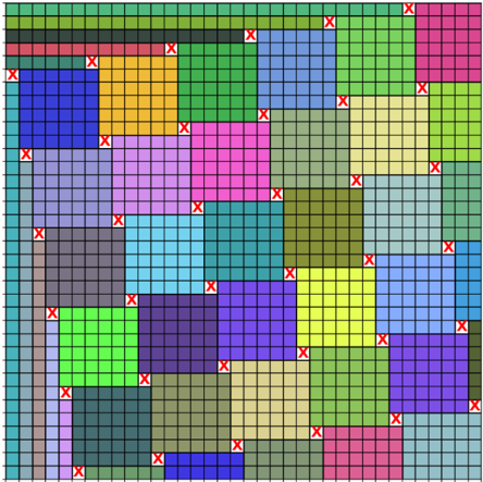
The image displays a 20x20 grid composed of 400 small, uniform squares. This grid is partitioned into 25 distinct, non-overlapping rectangular regions of varying sizes and colors. Each colored region is a contiguous block of grid squares. At the top-left corner of each colored region, a red 'X' marker is placed, seemingly indicating the origin or anchor point of that partition. There is no accompanying text, legend, axis labels, or numerical data.
### Components/Axes
* **Grid Structure:** A uniform 20x20 grid of small squares forms the base layer.
* **Partitions:** 25 rectangular regions of different colors and dimensions overlay the grid.
* **Markers:** Red 'X' symbols are placed at the top-left grid intersection of each colored region.
* **Colors:** The partitions use a diverse palette including shades of blue, green, yellow, pink, purple, gray, and teal. No two adjacent regions share the same color.
* **Text/Labels:** **None present.** The diagram is purely visual.
### Detailed Analysis
**Spatial Layout and Partitioning:**
The grid is densely packed with rectangular partitions. The regions vary significantly in size:
* **Largest Regions:** Appear to be approximately 6x6 or 7x5 grid squares (e.g., a large dark blue region in the top-left, a large pink region in the center).
* **Smallest Regions:** Are as small as 2x2 or 3x2 grid squares (e.g., a small dark blue region at the bottom-center, a small pink region at the bottom-right).
* **Arrangement:** The partitions are arranged in a seemingly irregular, non-repeating pattern. They tessellate the grid completely with no gaps or overlaps.
**Marker Placement:**
Each red 'X' is precisely positioned at the top-left corner of its respective colored rectangle. For example:
* The 'X' for the large dark blue region in the top-left is at grid coordinate (1,1) from the top-left.
* The 'X' for the large pink region in the center is at approximately (8,8).
* The 'X' for the small dark blue region at the bottom is at approximately (10,19).
**Color Distribution:**
Colors are distributed across the grid without an obvious gradient or pattern. Similar hues (e.g., different shades of green or blue) are often placed in non-adjacent regions.
### Key Observations
1. **Complete Tessellation:** The 25 rectangles perfectly cover the entire 20x20 grid area without any empty cells or overlaps.
2. **Irregular Sizing:** The partitions are not uniform; they range from large blocks to small slivers, suggesting a dynamic or data-driven allocation process.
3. **Boundary Markers:** The consistent placement of the red 'X' at the top-left corner of each region is the only standardized element, serving as a clear identifier for each partition's origin.
4. **Lack of Hierarchy:** There is no visual indication of hierarchy or relationship between the colored regions beyond their spatial adjacency.
### Interpretation
This diagram is a **visual representation of a spatial partitioning or allocation scheme**. The absence of text or a legend means the information is encoded purely in the geometry and color of the regions.
* **What it likely represents:** It could visualize the output of a **memory allocation algorithm** (showing how blocks of memory are assigned), a **domain decomposition method** in computational physics (splitting a problem space for parallel processing), a **clustering result** on a 2D grid, or a **resource map** where colors represent different types or owners of contiguous resources.
* **The 'X' markers** are critical. They define the "handle" or reference point for each allocated block, which is essential for algorithms that need to locate or manage these blocks.
* **The varying sizes** suggest the underlying data or requirements are heterogeneous. Some "processes" or "data clusters" require large contiguous spaces, while others are small.
* **The irregular pattern** indicates the partitioning is likely the result of an optimization or allocation process responding to specific constraints or input data, rather than a simple, regular grid division.
**In essence, the image conveys the *state* of a system after a partitioning operation. The key facts are the number of partitions (25), their precise locations and dimensions on the grid, and their assigned identifiers (via color and marker). To extract deeper meaning (e.g., what each color signifies), a legend or accompanying text would be required.**