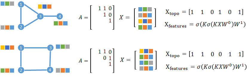
## Diagram: Graph Neural Network Feature and Topology Representation
### Overview
The image displays two parallel examples (top and bottom rows) illustrating the representation of graph structures, their adjacency matrices, feature matrices, and derived topological and feature-based vectors for graph neural networks. Each row shows a graph with 4 nodes, its corresponding adjacency matrix `A`, feature matrix `X`, a topological encoding vector `X_topo`, and a feature transformation formula `X_features`.
### Components/Axes
The image is divided into two distinct rows, each containing the following components from left to right:
1. **Graph Diagram**: A visual representation of a graph with numbered nodes (1-4) and edges connecting them. Each node is surrounded by colored squares representing feature vectors.
2. **Adjacency Matrix `A`**: A 4x4 matrix representing the graph's connectivity.
3. **Feature Matrix `X`**: A 4x3 matrix where each row corresponds to a node's feature vector (represented by colored squares).
4. **Topological Encoding `X_topo`**: A 1x6 binary vector.
5. **Feature Transformation `X_features`**: A mathematical formula.
### Detailed Analysis
#### **Top Row**
* **Graph Structure**:
* Nodes: 1, 2, 3, 4.
* Edges: (1-2), (1-3), (2-3), (3-4). This forms a triangle between nodes 1, 2, and 3, with node 4 connected only to node 3.
* Node Features (Colored Squares):
* Node 1: Top-left: Green, Grey. Top-right: Yellow, Blue, Orange.
* Node 2: Bottom-left: Grey, Orange, Blue.
* Node 3: Top-right: Yellow, Blue, Orange. Bottom-right: Green, Grey.
* Node 4: Bottom-right: Green, Grey, Orange.
* **Adjacency Matrix `A`**:
```
A = [ 1 1 0 ]
[ 1 0 1 ]
[ 1 ]
```
*Note: The matrix is presented in a sparse, upper-triangular-like format. The full 4x4 symmetric adjacency matrix implied is:*
```
[0 1 1 0]
[1 0 1 0]
[1 1 0 1]
[0 0 1 0]
```
* **Feature Matrix `X`**:
```
X = [ Green, Grey, ? ]
[ Yellow, Blue, Orange ]
[ Grey, Orange, Blue ]
[ Green, Grey, Orange ]
```
*Note: The matrix is represented visually with colored squares. The exact mapping of colors to numerical values is not provided. The first row (Node 1) has only two visible squares, suggesting a possible missing or zero-padded feature.*
* **Topological Encoding `X_topo`**:
`X_topo = [1 1 0 1 0 1]`
* **Feature Transformation `X_features`**:
`X_features = σ(Kσ(KXW⁰)W¹)`
#### **Bottom Row**
* **Graph Structure**:
* Nodes: 1, 2, 3, 4.
* Edges: (1-2), (1-3), (2-4), (3-4). This forms a square/cycle: 1-2-4-3-1.
* Node Features (Colored Squares):
* Node 1: Top-left: Yellow, Blue, Orange.
* Node 2: Bottom-left: Green, Orange, Blue.
* Node 3: Top-right: Green, Grey, Orange.
* Node 4: Bottom-right: Grey, Orange, Blue.
* **Adjacency Matrix `A`**:
```
A = [ 1 1 0 ]
[ 0 1 1 ]
[ 1 ]
```
*Note: The full 4x4 symmetric adjacency matrix implied is:*
```
[0 1 1 0]
[1 0 0 1]
[1 0 0 1]
[0 1 1 0]
```
* **Feature Matrix `X`**:
```
X = [ Yellow, Blue, Orange ]
[ Green, Orange, Blue ]
[ Green, Grey, Orange ]
[ Grey, Orange, Blue ]
```
* **Topological Encoding `X_topo`**:
`X_topo = [1 1 0 0 1 1]`
* **Feature Transformation `X_features`**:
`X_features = σ(Kσ(KXW⁰)W¹)` (Identical formula to the top row).
### Key Observations
1. **Graph Topology Difference**: The primary difference between the two examples is the graph structure. The top graph has a triangular core with a pendant node, while the bottom graph is a 4-node cycle.
2. **`X_topo` Variation**: The topological encoding vector `X_topo` changes between the two rows (`[1 1 0 1 0 1]` vs. `[1 1 0 0 1 1]`), reflecting the difference in graph connectivity. This vector likely encodes the presence or absence of specific subgraph patterns or edge types.
3. **Consistent Formula**: The feature transformation formula `X_features` is identical in both rows, indicating the same neural network operation is applied regardless of the underlying graph topology.
4. **Feature Representation**: Node features are represented abstractly by colored squares. The specific numerical meaning of each color (e.g., Green = 1, Grey = 0) is not defined in the image.
5. **Matrix Notation**: The adjacency matrices `A` are shown in a compact, sparse notation, listing only the non-zero entries in the upper triangle.
### Interpretation
This diagram serves as a conceptual illustration for Graph Neural Networks (GNNs). It demonstrates two fundamental components of graph data:
1. **Topology (`A`, `X_topo`)**: The structure of connections between entities (nodes). The `X_topo` vector is a learned or engineered representation of this structure, which differs based on whether the graph contains a triangle (top) or is a pure cycle (bottom).
2. **Node Features (`X`, `X_features`)**: The attributes associated with each entity. The formula `X_features = σ(Kσ(KXW⁰)W¹)` represents a typical GNN layer operation (like a graph convolution), where:
* `X` is the input feature matrix.
* `W⁰` and `W¹` are learnable weight matrices.
* `K` likely represents a graph convolution operator (e.g., involving the adjacency matrix `A`).
* `σ` is a non-linear activation function.
The image highlights that while the feature transformation mechanism (`X_features`) may be constant, the resulting node embeddings are inherently influenced by the distinct graph topologies, as captured by the different `X_topo` encodings. This is a core principle of GNNs: learning representations that integrate both attribute information and relational structure.