\n
## [Chart Type]: Dual-Panel Training Dynamics Plot
### Overview
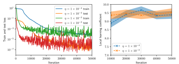
The image displays two side-by-side line charts analyzing the training dynamics of a machine learning model under two different learning rates (η). The left panel shows the training and test loss over iterations on a logarithmic scale. The right panel shows the "Local learning coefficient" over iterations on a linear scale. Both charts compare the same two learning rates: η = 1×10⁻⁴ and η = 1×10⁻³.
### Components/Axes
**Left Panel (Loss vs. Iteration):**
* **Y-axis:** Label: "Train and test loss". Scale: Logarithmic, ranging from 10⁻⁷ to 10¹.
* **X-axis:** Label: "Iteration". Scale: Linear, from 0 to 50,000.
* **Legend (Top-Left):** Contains four entries:
1. `η = 1 × 10⁻⁴ train` (Solid blue line)
2. `η = 1 × 10⁻⁴ test` (Solid orange line)
3. `η = 1 × 10⁻³ train` (Solid green line)
4. `η = 1 × 10⁻³ test` (Solid red line)
**Right Panel (Local Learning Coefficient vs. Iteration):**
* **Y-axis:** Label: "Local learning coefficient". Scale: Linear, from 7.0 to 10.0.
* **X-axis:** Label: "Iteration". Scale: Linear, from 10,000 to 50,000.
* **Legend (Bottom-Right):** Contains two entries:
1. `η = 1 × 10⁻⁴` (Blue dashed line with 'x' markers, shaded blue confidence interval)
2. `η = 1 × 10⁻³` (Orange dashed line with 'x' markers, shaded orange confidence interval)
### Detailed Analysis
**Left Panel - Loss Trends:**
* **η = 1×10⁻⁴ (Blue/Orange):** Both training (blue) and test (orange) loss start high (~10⁰ to 10¹). They show a steep, smooth decline until approximately iteration 10,000. After this point, the decline slows significantly. The training loss (blue) continues a steady, smooth decrease, reaching approximately 10⁻⁵ by iteration 50,000. The test loss (orange) follows a similar path but exhibits more noise/fluctuation and remains slightly above the training loss, ending near 10⁻⁴.
* **η = 1×10⁻³ (Green/Red):** Both losses start lower than the η=1×10⁻⁴ case. They drop extremely rapidly within the first few thousand iterations. The training loss (green) stabilizes into a very noisy band between approximately 10⁻³ and 10⁻⁴. The test loss (red) is the noisiest series, fluctuating wildly in a band between 10⁻⁵ and 10⁻⁷, and is consistently lower than its corresponding training loss, which is an unusual pattern.
**Right Panel - Local Learning Coefficient Trends:**
* **η = 1×10⁻⁴ (Blue):** The coefficient starts at approximately 8.8 at iteration 10,000. It shows a clear upward trend, peaking at about 9.7 around iteration 30,000, before slightly declining and stabilizing around 9.5 by iteration 50,000. The shaded confidence interval is relatively narrow.
* **η = 1×10⁻³ (Orange):** The coefficient starts higher, at approximately 9.3 at iteration 10,000. It follows a similar upward trend but is consistently lower than the η=1×10⁻⁴ line after the initial point. It peaks at about 9.5 around iteration 25,000 and then gently declines to approximately 9.3 by iteration 50,000. Its confidence interval is wider than the blue line's, indicating higher variance.
### Key Observations
1. **Learning Rate Impact on Loss:** The higher learning rate (η=1×10⁻³) leads to much faster initial loss reduction but results in higher final loss values and significantly more noise (instability) in both training and test loss compared to the lower learning rate (η=1×10⁻⁴).
2. **Unusual Test/Train Loss Relationship:** For η=1×10⁻³, the test loss (red) is consistently and significantly *lower* than the training loss (green). This is atypical and could indicate issues like data leakage, a non-representative test set, or a specific regularization effect.
3. **Learning Coefficient Evolution:** The local learning coefficient increases for both learning rates during the observed window (10k-50k iterations), suggesting the model is moving through a region of the loss landscape where parameters are becoming more sensitive. The lower learning rate maintains a higher coefficient value.
4. **Noise Correlation:** The high noise in the loss curves for η=1×10⁻³ correlates with the wider confidence interval (higher variance) in its local learning coefficient measurement.
### Interpretation
This data provides a technical comparison of optimization dynamics. The **lower learning rate (η=1×10⁻⁴)** demonstrates more stable, controlled convergence: it achieves lower final loss with smooth curves and a higher, more stable local learning coefficient, suggesting it is navigating the loss landscape more precisely. The **higher learning rate (η=1×10⁻³)** causes aggressive, noisy optimization. While it reduces loss quickly initially, it fails to settle into a deep minimum (higher final loss) and exhibits erratic behavior, as seen in the noisy loss bands and the lower, more variable learning coefficient.
The anomalous test loss being lower than training loss for the high learning rate is a critical red flag for investigation. It challenges the standard expectation that training loss should be lower and could imply the test set is easier than the training set, or that the high learning rate is acting as a strong implicit regularizer that benefits generalization more than in-distribution fitting in a non-standard way.
The rising local learning coefficient for both rates indicates the training process is not in a simple, flat region of the loss landscape; the model's parameters remain sensitive to updates even after 50,000 iterations. The fact that the lower learning rate maintains a higher coefficient suggests it is preserving more "learnability" or is positioned in a more curved region of the loss landscape.