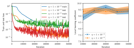
\n ## Charts: Training and Test Loss vs. Iteration & Local Learning Coefficient vs. Iteration ### Overview The image presents two charts side-by-side. The left chart displays the training and test loss as a function of iteration for two different learning rates (η = 1 x 10⁻⁴ and η = 1 x 10⁻³). The right chart shows the local learning coefficient as a function of iteration, also for the same two learning rates. Both charts aim to illustrate the training dynamics of a model. ### Components/Axes **Left Chart:** * **X-axis:** Iteration (Scale: 0 to 50000, logarithmic scale) * **Y-axis:** Train and test loss (Scale: 10⁻¹ to 10⁰, logarithmic scale) * **Legend:** * Blue Line: η = 1 x 10⁻⁴ train * Red Line: η = 1 x 10⁻⁴ test * Green Line: η = 1 x 10⁻³ train * Orange Line: η = 1 x 10⁻³ test **Right Chart:** * **X-axis:** Iteration (Scale: 0 to 50000) * **Y-axis:** Local learning coefficient (Scale: 7.0 to 10.0) * **Legend:** * Blue Dashed Line with 'x' Markers: η = 1 x 10⁻⁴ * Orange Dashed Line with '+' Markers: η = 1 x 10⁻³ ### Detailed Analysis or Content Details **Left Chart:** * **η = 1 x 10⁻⁴ (Blue & Red):** The blue 'train' line starts at approximately 0.9 and decreases rapidly to around 0.01 by iteration 10000. It then fluctuates around 0.01 to 0.005 for the remainder of the iterations. The red 'test' line starts at approximately 0.9 and initially decreases, but remains significantly higher than the blue line, fluctuating between 0.02 and 0.08 throughout the iterations. * **η = 1 x 10⁻³ (Green & Orange):** The green 'train' line starts at approximately 0.9 and decreases more quickly than the blue line, reaching around 0.001 by iteration 10000. It continues to decrease, but with more fluctuations, reaching approximately 0.0005 by iteration 50000. The orange 'test' line starts at approximately 0.9 and initially decreases, but quickly plateaus and fluctuates around 0.05 to 0.15 for the majority of the iterations. **Right Chart:** * **η = 1 x 10⁻⁴ (Blue):** The blue line starts at approximately 9.6 at iteration 0, decreases to a minimum of around 8.2 at iteration 20000, and then increases again, fluctuating between 9.2 and 9.7 for the remainder of the iterations. The shaded area around the line represents the standard deviation or confidence interval. * **η = 1 x 10⁻³ (Orange):** The orange line starts at approximately 9.6 at iteration 0, decreases to a minimum of around 8.0 at iteration 20000, and then increases again, fluctuating between 9.0 and 9.6 for the remainder of the iterations. The shaded area around the line represents the standard deviation or confidence interval. ### Key Observations * The learning rate of 1 x 10⁻³ results in a lower training loss compared to 1 x 10⁻⁴, but the test loss remains significantly higher. * The test loss for both learning rates plateaus at a higher value than the training loss, indicating potential overfitting. * The local learning coefficient fluctuates around a value of 9.5 for both learning rates, with some variation over iterations. * The local learning coefficient appears to decrease initially and then stabilize. ### Interpretation The charts demonstrate the impact of different learning rates on the training and generalization performance of a model. The lower learning rate (1 x 10⁻⁴) leads to a smoother training process but struggles to achieve a low test loss, suggesting underfitting or slow convergence. The higher learning rate (1 x 10⁻³) achieves a lower training loss more quickly, but the higher test loss indicates overfitting. The local learning coefficient provides insight into the adaptive learning process, showing how the learning rate is adjusted during training. The fluctuations in the local learning coefficient suggest that the optimization algorithm is dynamically adapting to the loss landscape. The shaded areas in the right chart indicate the uncertainty or variability in the local learning coefficient, which could be due to stochasticity in the training process or the inherent complexity of the model. The divergence between training and test loss suggests that regularization techniques or a larger dataset might be needed to improve generalization performance.