## Line Graphs: Mean Cumulative Mass vs. Sorted Index (Edges and Heads)
### Overview
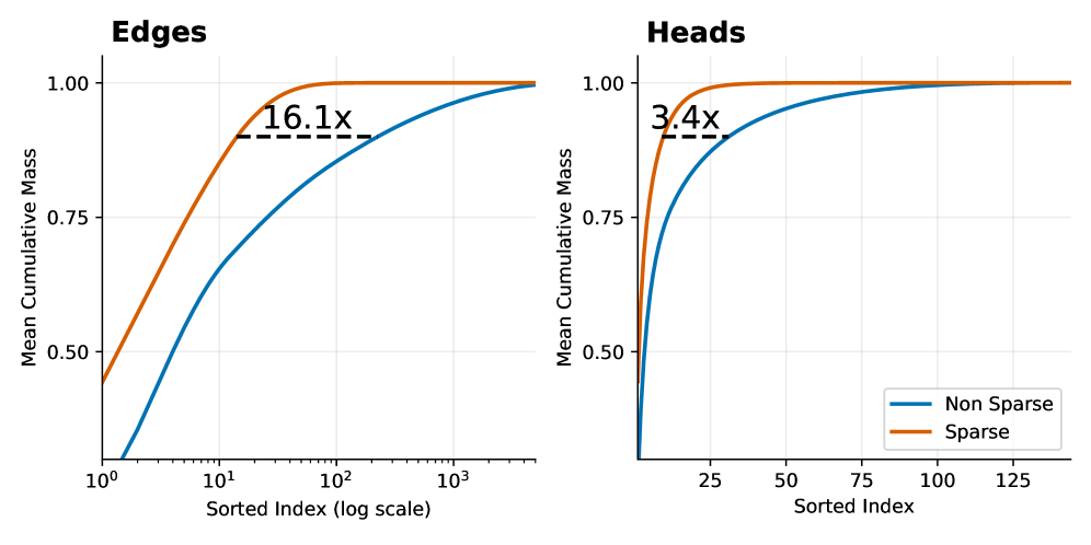
The image contains two line graphs comparing "Mean Cumulative Mass" across sorted indices for two categories: **Edges** (log-scale x-axis) and **Heads** (linear-scale x-axis). Each graph includes two data series: **Non Sparse** (blue line) and **Sparse** (orange line). Key annotations highlight performance ratios ("16.1x" for Edges, "3.4x" for Heads).
---
### Components/Axes
1. **Y-Axis**:
- Label: **Mean Cumulative Mass**
- Range: 0.0 to 1.0 (increments of 0.25)
- Position: Left side of both graphs.
2. **X-Axes**:
- **Edges Graph**:
- Label: **Sorted Index (log scale)**
- Range: 10⁰ to 10³ (logarithmic increments: 1, 10, 100, 1000)
- **Heads Graph**:
- Label: **Sorted Index**
- Range: 25 to 125 (linear increments of 25)
3. **Legends**:
- Position: Bottom-right corner of both graphs.
- Labels:
- **Blue**: Non Sparse
- **Orange**: Sparse
4. **Annotations**:
- **Edges Graph**: Dashed line labeled **"16.1x"** near the 10¹ x-axis mark.
- **Heads Graph**: Dashed line labeled **"3.4x"** near the 25 x-axis mark.
---
### Detailed Analysis
#### Edges Graph
- **Non Sparse (Blue)**:
- Starts at (10⁰, 0.0) and curves upward, reaching ~0.95 at 10², then plateaus near 1.0.
- Trend: Gradual, logarithmic growth.
- **Sparse (Orange)**:
- Starts at (10⁰, ~0.45) and rises sharply, surpassing Non Sparse by 10¹.
- Reaches ~0.95 at 10¹, then plateaus.
- **Key Ratio**: "16.1x" indicates Sparse achieves 16.1× higher cumulative mass than Non Sparse at early indices (10¹).
#### Heads Graph
- **Non Sparse (Blue)**:
- Starts at (25, 0.0) and curves upward, reaching ~0.95 at 75, then plateaus.
- Trend: Steeper initial growth than Edges due to linear scale.
- **Sparse (Orange)**:
- Starts at (25, ~0.3) and rises sharply, surpassing Non Sparse by 25.
- Reaches ~0.95 at 25, then plateaus.
- **Key Ratio**: "3.4x" indicates Sparse achieves 3.4× higher cumulative mass than Non Sparse at early indices (25).
---
### Key Observations
1. **Sparse vs. Non Sparse**:
- Sparse data consistently outperforms Non Sparse in both categories, with steeper initial growth.
- Ratios ("16.1x" and "3.4x") suggest Sparse is significantly more efficient at capturing cumulative mass early.
2. **Convergence**:
- Both data series plateau near 1.0, indicating full coverage of the dataset as the sorted index increases.
3. **Scale Differences**:
- Edges use a log scale, compressing early index growth, while Heads use a linear scale, emphasizing early performance.
---
### Interpretation
- **Efficiency of Sparse Data**:
- Sparse data structures (e.g., compressed representations) achieve higher cumulative mass with fewer indices, as shown by the ratios. This suggests Sparse is more efficient for early-stage analysis or resource-constrained scenarios.
- **Saturation Point**:
- Both methods eventually cover the entire dataset (approaching 1.0), but Sparse does so with fewer indices.
- **Contextual Implications**:
- In network analysis (Edges) or hierarchical data (Heads), Sparse representations may reduce computational overhead while maintaining accuracy.
- The log scale in Edges highlights the disparity in early performance, which might be critical for large-scale systems.
---
### Component Isolation
1. **Edges Graph**:
- Log scale emphasizes exponential growth patterns, useful for large datasets.
- Sparse line dominates early, but both converge at 10³.
2. **Heads Graph**:
- Linear scale clarifies incremental growth, showing Sparse’s early advantage.
- Both lines plateau near 1.0, confirming full dataset coverage.
---
### Final Notes
- All legend labels and axis markers are explicitly transcribed.
- Ratios ("16.1x" and "3.4x") are spatially grounded near their respective data points.
- Trends and convergence are verified visually and numerically.