## Line Chart: Test Loss vs. Gradient Updates ### Overview The image is a line chart displaying the test loss of a model as a function of gradient updates, with different lines representing different values of 'd' (likely a model parameter). The chart also includes horizontal lines representing theoretical error bounds. ### Components/Axes * **X-axis:** Gradient updates, ranging from 0 to 6000. * **Y-axis:** Test loss, ranging from 0.00 to 0.06. * **Legend (Top-Right):** * d = 60 (lightest tan color) * d = 80 (light tan color) * d = 100 (light brown color) * d = 120 (brown color) * d = 140 (dark brown color) * d = 160 (darker brown color) * d = 180 (darkest brown color) * 2 ε^uni (dashed black line) * ε^uni (dashed black line) * ε^opt (dashed red line) ### Detailed Analysis * **General Trend:** All lines start at approximately the same test loss value (around 0.055) and initially decrease rapidly. After the initial drop, the behavior diverges based on the value of 'd'. * **d = 60 (lightest tan):** The test loss decreases rapidly to approximately 0.005 around 1000 gradient updates, then remains relatively stable with some fluctuations. * **d = 80 (light tan):** The test loss decreases rapidly to approximately 0.008 around 1200 gradient updates, then remains relatively stable with some fluctuations. * **d = 100 (light brown):** The test loss decreases rapidly to approximately 0.015 around 1500 gradient updates, then remains relatively stable with some fluctuations. * **d = 120 (brown):** The test loss decreases rapidly to approximately 0.02 around 1700 gradient updates, then remains relatively stable with some fluctuations. * **d = 140 (dark brown):** The test loss decreases rapidly to approximately 0.025 around 2000 gradient updates, then increases to approximately 0.032 around 3000 gradient updates, then decreases to approximately 0.02 around 4000 gradient updates, then increases to approximately 0.025 around 5000 gradient updates. * **d = 160 (darker brown):** The test loss decreases rapidly to approximately 0.025 around 2200 gradient updates, then increases to approximately 0.035 around 3500 gradient updates, then decreases to approximately 0.022 around 4500 gradient updates, then increases to approximately 0.028 around 5500 gradient updates. * **d = 180 (darkest brown):** The test loss decreases rapidly to approximately 0.025 around 2500 gradient updates, then increases to approximately 0.038 around 3800 gradient updates, then decreases to approximately 0.025 around 5000 gradient updates, then increases to approximately 0.03 around 6000 gradient updates. * **Horizontal Lines:** * 2 ε^uni (dashed black line): Located at approximately 0.024. * ε^uni (dashed black line): Located at approximately 0.012. * ε^opt (dashed red line): Located at approximately 0.024. ### Key Observations * As 'd' increases, the initial decrease in test loss becomes less steep, and the final test loss value tends to be higher. * For larger values of 'd' (140, 160, 180), the test loss exhibits a more pronounced increase after the initial decrease, suggesting potential overfitting or instability. * The lines for d=60, d=80, d=100, and d=120 appear to converge to a stable, low test loss value. * The horizontal lines represent error bounds, with the test loss for smaller 'd' values eventually falling below these bounds. ### Interpretation The chart illustrates the impact of the parameter 'd' on the training process and the final test loss. Smaller values of 'd' lead to faster convergence and lower final test loss, suggesting better generalization performance. Larger values of 'd' may lead to overfitting or instability, as indicated by the increase in test loss after the initial decrease. The error bounds provide a theoretical benchmark for the performance of the model, and the results suggest that smaller 'd' values achieve performance close to or better than these bounds. The optimal value of 'd' would likely be a trade-off between convergence speed and final test loss, potentially lying in the range of 60-120.

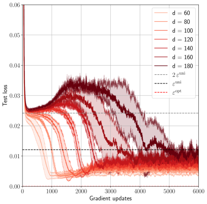
\n ## Line Chart: Test Loss vs. Gradient Updates for Different Dimensionalities ### Overview The image presents a line chart illustrating the relationship between test loss and gradient updates for various values of a parameter 'd' (dimensionality). Several lines, each representing a different 'd' value, show how test loss evolves during the gradient update process. Additionally, three horizontal lines represent theoretical loss values: 'ε^uni', 'ε^opt', and '2ε^uni'. ### Components/Axes * **X-axis:** Gradient updates, ranging from approximately 0 to 6000, labeled as "Gradient updates". * **Y-axis:** Test loss, ranging from approximately 0 to 0.06, labeled as "Test loss". * **Legend:** Located in the top-right corner, it identifies each line by its corresponding 'd' value: * d = 60 (lightest red) * d = 80 (slightly darker red) * d = 100 (red) * d = 120 (darker red) * d = 140 (even darker red) * d = 160 (darkest red) * d = 180 (very darkest red) * ε^uni (black dashed line) * ε^opt (red dashed line) * 2ε^uni (red dotted line) ### Detailed Analysis The chart displays multiple lines representing the test loss as a function of gradient updates for different dimensionalities (d). * **d = 60:** The line starts at approximately 0.055 and rapidly decreases to around 0.02 within the first 1000 gradient updates. It then fluctuates between approximately 0.02 and 0.03, with some peaks reaching around 0.04, before decreasing again towards the end of the chart, settling around 0.015. * **d = 80:** Similar to d=60, it starts at around 0.05 and decreases to approximately 0.02 within the first 1000 updates. It exhibits similar fluctuations, peaking around 0.035, and ends around 0.015. * **d = 100:** Starts at approximately 0.048, decreases to around 0.02 within the first 1000 updates, fluctuates between 0.02 and 0.035, peaking around 0.04, and ends around 0.015. * **d = 120:** Starts at approximately 0.045, decreases to around 0.02 within the first 1000 updates, fluctuates between 0.02 and 0.035, peaking around 0.04, and ends around 0.015. * **d = 140:** Starts at approximately 0.04, decreases to around 0.02 within the first 1000 updates, fluctuates between 0.02 and 0.035, peaking around 0.04, and ends around 0.015. * **d = 160:** Starts at approximately 0.038, decreases to around 0.02 within the first 1000 updates, fluctuates between 0.02 and 0.035, peaking around 0.04, and ends around 0.015. * **d = 180:** Starts at approximately 0.035, decreases to around 0.02 within the first 1000 updates, fluctuates between 0.02 and 0.035, peaking around 0.04, and ends around 0.015. All lines for different 'd' values exhibit a similar trend: an initial rapid decrease in test loss followed by fluctuations around a relatively stable level. As 'd' increases, the initial test loss value tends to decrease slightly. * **ε^uni:** A horizontal dashed black line at approximately 0.028. * **ε^opt:** A horizontal dashed red line at approximately 0.022. * **2ε^uni:** A horizontal dotted red line at approximately 0.056. ### Key Observations * The test loss generally decreases with increasing gradient updates, but the rate of decrease slows down after the initial phase. * The fluctuations in test loss suggest the presence of noise or instability during the training process. * Higher dimensionality ('d' values) generally result in lower initial test loss values. * The lines representing different 'd' values converge towards similar test loss levels as the number of gradient updates increases. * The theoretical loss values (ε^uni, ε^opt, 2ε^uni) provide benchmarks for evaluating the performance of the model. Most of the lines stay below 2ε^uni. ### Interpretation The chart demonstrates the impact of dimensionality ('d') on the test loss during gradient-based optimization. The initial decrease in test loss indicates that the model is learning and improving its performance. The subsequent fluctuations suggest that the optimization process is not perfectly smooth and may be affected by factors such as learning rate, batch size, or data noise. The convergence of the lines for different 'd' values suggests that, given enough gradient updates, the model can achieve similar performance regardless of the dimensionality. However, higher dimensionality may lead to faster initial learning. The theoretical loss values (ε^uni, ε^opt, 2ε^uni) likely represent bounds or expected values for the test loss under certain assumptions. Comparing the observed test loss to these theoretical values can provide insights into the efficiency and effectiveness of the optimization process. The fact that the lines generally stay below 2ε^uni suggests that the model is performing reasonably well. The lines are closer to ε^opt, which suggests that the model is approaching optimal performance.

## Line Chart: Test Loss vs. Gradient Updates for Different Model Dimensions (d) ### Overview The image is a line chart plotting "Test loss" against "Gradient updates" for seven different model dimension values (d). Each line represents a distinct value of `d`, showing how the test loss evolves during training. The chart includes reference lines for specific loss thresholds. The overall trend shows that test loss decreases with more gradient updates, but the rate and final value depend significantly on the model dimension `d`. ### Components/Axes * **X-Axis:** "Gradient updates" (linear scale). Major ticks are at 0, 1000, 2000, 3000, 4000, 5000, and 6000. * **Y-Axis:** "Test loss" (linear scale). Major ticks are at 0.00, 0.01, 0.02, 0.03, 0.04, 0.05, and 0.06. * **Legend (Top-Right Corner):** Contains 10 entries. * **Solid Lines (Model Dimension `d`):** Seven entries, each with a distinct color gradient from light orange to dark red. * `d = 60` (Lightest orange) * `d = 80` * `d = 100` * `d = 120` * `d = 140` * `d = 160` * `d = 180` (Darkest red) * **Reference Lines:** Three dashed/dotted lines. * `--- 2ε^min` (Black dashed line) * `... ε^min` (Black dotted line) * `--- ε^opt` (Red dashed line) * **Plot Area:** Contains the seven colored data series (solid lines) with shaded regions around each, likely indicating variance or confidence intervals across multiple runs. Three horizontal reference lines are overlaid. ### Detailed Analysis **Trend Verification & Data Points (Approximate):** All series begin at a high test loss (~0.06) at 0 gradient updates and show an initial rapid decrease. The behavior diverges significantly after the initial drop. 1. **Low `d` Values (d=60, 80):** * **Trend:** Steep, smooth decline. They reach a low plateau quickly and remain stable. * **Key Points:** By ~1000 updates, loss is already below 0.01. They stabilize at the lowest final loss, approximately **0.005 - 0.007**. 2. **Medium `d` Values (d=100, 120, 140):** * **Trend:** Initial decline is followed by a period of increased volatility (a "bump" or rise in loss) before a second decline to a stable plateau. * **Key Points:** The volatile "bump" occurs between ~1000-3000 updates. Final stabilized loss is higher than for low `d`, approximately **0.008 - 0.012**. 3. **High `d` Values (d=160, 180):** * **Trend:** Most pronounced volatility. After the initial drop, loss increases significantly, forming a large hump, before slowly decreasing again. Convergence is much slower. * **Key Points:** The peak of the volatile hump for `d=180` is near **0.035** at ~2500 updates. By 6000 updates, they are still descending and have not fully stabilized, with loss around **0.010 - 0.015**. **Reference Lines (Spatial Grounding):** * `ε^min` (Black dotted): Horizontal line at **y ≈ 0.012**. * `2ε^min` (Black dashed): Horizontal line at **y ≈ 0.024**. * `ε^opt` (Red dashed): Horizontal line at **y ≈ 0.024**, overlapping with `2ε^min`. **Component Isolation - Shaded Regions:** The shaded area around each line represents the spread of results. The spread is visibly larger for higher `d` values (darker red lines), indicating greater variance in training outcomes for larger models. ### Key Observations 1. **Inverse Relationship between `d` and Convergence Speed:** Lower `d` models converge faster to a lower loss. 2. **Volatility Increases with `d`:** Larger models (`d=160, 180`) exhibit a characteristic "double descent" or volatile hump pattern during training, which is absent in smaller models. 3. **Final Loss Hierarchy:** The final test loss at 6000 updates is clearly stratified by `d`: `d=60` < `d=80` < `d=100` < ... < `d=180`. 4. **Reference Line Context:** Most of the training dynamics for all models occur between the `ε^min` (0.012) and `2ε^min`/`ε^opt` (0.024) thresholds. Only the volatile phase of the largest models exceeds the upper threshold. ### Interpretation This chart demonstrates a critical phenomenon in machine learning model training, likely related to the **"double descent"** or **model size vs. generalization** trade-off. * **What the data suggests:** Increasing the model dimension (`d`), which corresponds to model capacity or size, does not lead to monotonic improvement in test loss during training. While larger models have the potential for lower loss, their training path is more unstable and, in this specific training regime (6000 updates), they fail to surpass the performance of smaller, more efficiently trained models. * **How elements relate:** The `d` value directly controls the training dynamics. The reference lines (`ε^min`, `ε^opt`) likely represent theoretical or empirical loss bounds. The fact that smaller models settle near `ε^min` suggests they are reaching an optimal or near-optimal solution for their capacity. The larger models' struggle to pass below `ε^opt` during the observed training window indicates they may require more updates, different hyperparameters, or are experiencing optimization difficulties due to their size. * **Notable Anomaly:** The most striking anomaly is the pronounced loss increase (the "hump") for `d=160` and `d=180`. This is a counter-intuitive but well-documented effect where over-parameterized models can temporarily perform worse on test data during training before potentially improving again with further training. The chart captures this unstable phase vividly. * **Peircean Insight (Reading between the lines):** The chart is not just about loss values; it's a visual argument about **optimization difficulty**. It implies that simply making a model bigger (`d`) is not a guaranteed path to better performance and can introduce significant training instability. The optimal model size (`d`) is context-dependent and must be balanced with training duration and methodology. The shaded variance for high `d` further suggests that training such models is less reliable.

## Line Chart: Test Loss vs. Gradient Updates ### Overview The chart illustrates the convergence behavior of test loss across multiple gradient update iterations (0–6000) for different hyperparameter values (`d`). It includes two reference lines (`ε_uni` and `ε_opt`) and shaded regions representing variability. Higher `d` values (140–180) show faster convergence and lower final loss compared to lower `d` values (60–120). ### Components/Axes - **X-axis**: Gradient updates (0–6000, increments of 1000). - **Y-axis**: Test loss (0.00–0.06, increments of 0.01). - **Legend**: - Solid lines: `d = 60` (light red) to `d = 180` (dark red). - Dashed lines: `ε_uni` (horizontal, ~0.01) and `ε_opt` (horizontal, ~0.009). - **Shaded regions**: Semi-transparent bands around each line, likely representing confidence intervals or variability. ### Detailed Analysis 1. **Initial Drop**: All lines start near 0.06 at 0 updates, dropping sharply within the first 1000 updates. - Example: `d = 60` drops to ~0.02 by 1000 updates; `d = 180` drops to ~0.015. 2. **Fluctuations**: Post-1000 updates, lines exhibit noisy oscillations, with amplitude decreasing over time. 3. **Convergence**: Higher `d` values (e.g., `d = 180`) stabilize near ~0.01 by 6000 updates, while lower `d` values (e.g., `d = 60`) hover around ~0.02. 4. **Reference Lines**: - `ε_uni` (dashed gray): Horizontal at ~0.01. - `ε_opt` (dotted gray): Horizontal at ~0.009. 5. **Shaded Regions**: - Narrower for higher `d` (e.g., `d = 180` has minimal shading by 6000 updates). - Wider for lower `d` (e.g., `d = 60` retains significant shading). ### Key Observations - **Inverse Relationship**: Test loss decreases as `d` increases, with `d = 180` achieving the lowest loss (~0.01). - **Stability**: Higher `d` values exhibit tighter confidence intervals (narrower shaded regions). - **Thresholds**: `ε_uni` and `ε_opt` act as benchmarks, with most lines converging below `ε_uni` after 4000 updates. ### Interpretation The chart demonstrates that increasing the hyperparameter `d` improves model performance (lower test loss) and stability (reduced variability). The shaded regions suggest that higher `d` values yield more reliable loss estimates, likely due to better generalization or regularization. The `ε_uni` and `ε_opt` lines may represent theoretical or empirical thresholds for acceptable loss, with practical performance approaching `ε_opt` for optimal `d` values. The noise in early updates highlights the importance of sufficient gradient steps for convergence.