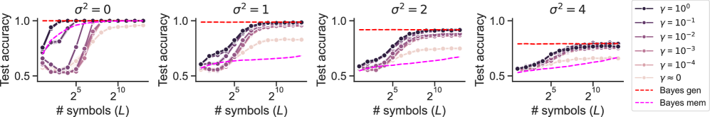
## Multi-Panel Line Chart: Test Accuracy vs. Number of Symbols under Varying Noise Levels ### Overview The image displays a series of four line charts arranged horizontally. Each chart plots "Test accuracy" on the y-axis against the "# symbols (L)" on the x-axis (logarithmic scale). The four panels represent experiments conducted under different noise levels, denoted by σ² (sigma squared), with values of 0, 1, 2, and 4 from left to right. Each panel contains multiple data series corresponding to different values of a regularization parameter γ (gamma), along with two baseline performance lines labeled "Bayes gen" and "Bayes mem". ### Components/Axes * **Panels:** Four distinct plots, each titled with its noise level: `σ² = 0`, `σ² = 1`, `σ² = 2`, `σ² = 4`. * **Y-Axis (All Panels):** Label: `Test accuracy`. Scale: Linear, ranging from 0.5 to 1.0. Major ticks are at 0.5 and 1.0. * **X-Axis (All Panels):** Label: `# symbols (L)`. Scale: Logarithmic (base 2). Major ticks are labeled at `2^5` (32) and `2^10` (1024). The axis spans approximately from 2^0 (1) to 2^12 (4096). * **Legend (Located to the right of the fourth panel):** * **Data Series (Solid lines with circular markers):** * `γ = 10^0` (Dark purple/black) * `γ = 10^-1` (Dark purple) * `γ = 10^-2` (Medium purple) * `γ = 10^-3` (Light purple) * `γ = 10^-4` (Lighter purple/pink) * `γ = 0` (Light pink) * **Baseline Series (Dashed lines):** * `Bayes gen` (Red dashed line) * `Bayes mem` (Magenta/pink dashed line) ### Detailed Analysis **Panel 1: σ² = 0 (No Noise)** * **Trend:** All models achieve high accuracy (>0.9) as the number of symbols (L) increases. The convergence speed depends heavily on γ. * **Data Points (Approximate):** * `γ = 10^0` and `γ = 10^-1`: Reach near-perfect accuracy (~1.0) very quickly, by L ≈ 2^3 (8). * `γ = 10^-2`: Reaches ~1.0 by L ≈ 2^5 (32). * `γ = 10^-3`: Reaches ~1.0 by L ≈ 2^7 (128). * `γ = 10^-4`: Reaches ~0.98 by L ≈ 2^10 (1024). * `γ = 0`: Shows a distinct dip in accuracy at low L (minimum ~0.6 at L≈2^2), then recovers to ~0.95 by L≈2^10. * `Bayes gen` (Red dashed): Constant at 1.0. * `Bayes mem` (Magenta dashed): Not visible/plotted in this panel, likely coincides with the top axis or is not applicable. **Panel 2: σ² = 1 (Low Noise)** * **Trend:** All models show reduced final accuracy compared to the noiseless case. Higher γ values lead to faster convergence but potentially lower asymptotic performance. * **Data Points (Approximate):** * `γ = 10^0`: Converges fastest, plateauing at ~0.95 by L≈2^7. * `γ = 10^-1`: Plateaus at ~0.95 by L≈2^8. * `γ = 10^-2`: Plateaus at ~0.93 by L≈2^9. * `γ = 10^-3`: Plateaus at ~0.88 by L≈2^10. * `γ = 10^-4`: Plateaus at ~0.82 by L≈2^11. * `γ = 0`: Shows a shallow dip, then slowly rises to ~0.75 by L≈2^11. * `Bayes gen` (Red dashed): Constant at ~0.98. * `Bayes mem` (Magenta dashed): Constant at ~0.65. **Panel 3: σ² = 2 (Medium Noise)** * **Trend:** Performance degradation continues. The gap between high-γ and low-γ models widens. The `Bayes mem` baseline becomes more relevant. * **Data Points (Approximate):** * `γ = 10^0`: Plateaus at ~0.90 by L≈2^8. * `γ = 10^-1`: Plateaus at ~0.88 by L≈2^9. * `γ = 10^-2`: Plateaus at ~0.85 by L≈2^10. * `γ = 10^-3`: Plateaus at ~0.78 by L≈2^11. * `γ = 10^-4`: Plateaus at ~0.70 by L≈2^11. * `γ = 0`: Rises slowly to ~0.65 by L≈2^11. * `Bayes gen` (Red dashed): Constant at ~0.92. * `Bayes mem` (Magenta dashed): Constant at ~0.60. **Panel 4: σ² = 4 (High Noise)** * **Trend:** All models struggle. Final accuracies are significantly lower. The benefit of increasing L diminishes for low-γ models. * **Data Points (Approximate):** * `γ = 10^0`: Plateaus at ~0.82 by L≈2^9. * `γ = 10^-1`: Plateaus at ~0.80 by L≈2^10. * `γ = 10^-2`: Plateaus at ~0.75 by L≈2^10. * `γ = 10^-3`: Plateaus at ~0.68 by L≈2^11. * `γ = 10^-4`: Plateaus at ~0.62 by L≈2^11. * `γ = 0`: Rises very slowly to ~0.58 by L≈2^11. * `Bayes gen` (Red dashed): Constant at ~0.80. * `Bayes mem` (Magenta dashed): Constant at ~0.55. ### Key Observations 1. **Noise Impact:** Increasing noise (σ²) universally reduces the maximum achievable test accuracy for all models and baselines. 2. **Regularization (γ) Effect:** Higher γ values (stronger regularization) lead to faster learning (steeper initial slope) and better robustness to noise, as seen by their higher plateau in noisy conditions (σ²=2,4). However, in the noiseless case (σ²=0), very high γ (`10^0`) converges quickly but all high-γ models perform similarly at the top. 3. **Pathological Case (γ=0):** The model with no regularization (`γ=0`) performs worst in all scenarios. In the noiseless case, it exhibits a characteristic "U-shaped" learning curve, initially getting worse before improving. 4. **Baselines:** The `Bayes gen` (generalization) line represents an upper bound that decreases with noise. The `Bayes mem` (memorization) line represents a lower bound that also decreases with noise. The gap between these baselines narrows as noise increases. 5. **Data Efficiency:** For a fixed noise level, achieving a target accuracy requires exponentially more symbols (L) as γ decreases. For example, at σ²=1, reaching 0.9 accuracy requires L≈2^6 for γ=10^0 but L>2^10 for γ=10^-3. ### Interpretation This chart demonstrates the **bias-variance tradeoff** in the context of learning from symbolic data under noise. The parameter γ controls model complexity/regularization. * **High γ (High Bias, Low Variance):** These models learn simple patterns quickly and are robust to noise, as they are less likely to fit the noise. Their performance plateaus earlier but at a higher level in noisy environments. * **Low γ (Low Bias, High Variance):** These models are more complex and can fit intricate patterns. In noiseless data, they eventually reach perfect accuracy but require more data (symbols). In noisy data, they are prone to overfitting the noise, leading to poorer generalization and lower final accuracy, as seen by their performance falling below the `Bayes gen` bound and sometimes approaching the `Bayes mem` bound. * **The γ=0 case** is an extreme of low bias/high variance, where the model initially fits noise (causing the accuracy dip) before learning the true signal with enough data. * The **Bayes baselines** provide theoretical benchmarks. The fact that models with appropriate regularization (e.g., γ=10^-1, 10^-2) can approach the `Bayes gen` line suggests they are achieving near-optimal generalization for the given noise level. The convergence of all models towards the `Bayes mem` line at very low L suggests that with insufficient data, all models are essentially memorizing. **In summary, the visualization argues for the necessity of regularization (γ > 0) to achieve robust and data-efficient learning, especially in the presence of noise. The optimal γ is noise-dependent: stronger regularization is beneficial as noise increases.**