## Histograms: Inner Product Distortion Distribution by Bitwidth
### Overview
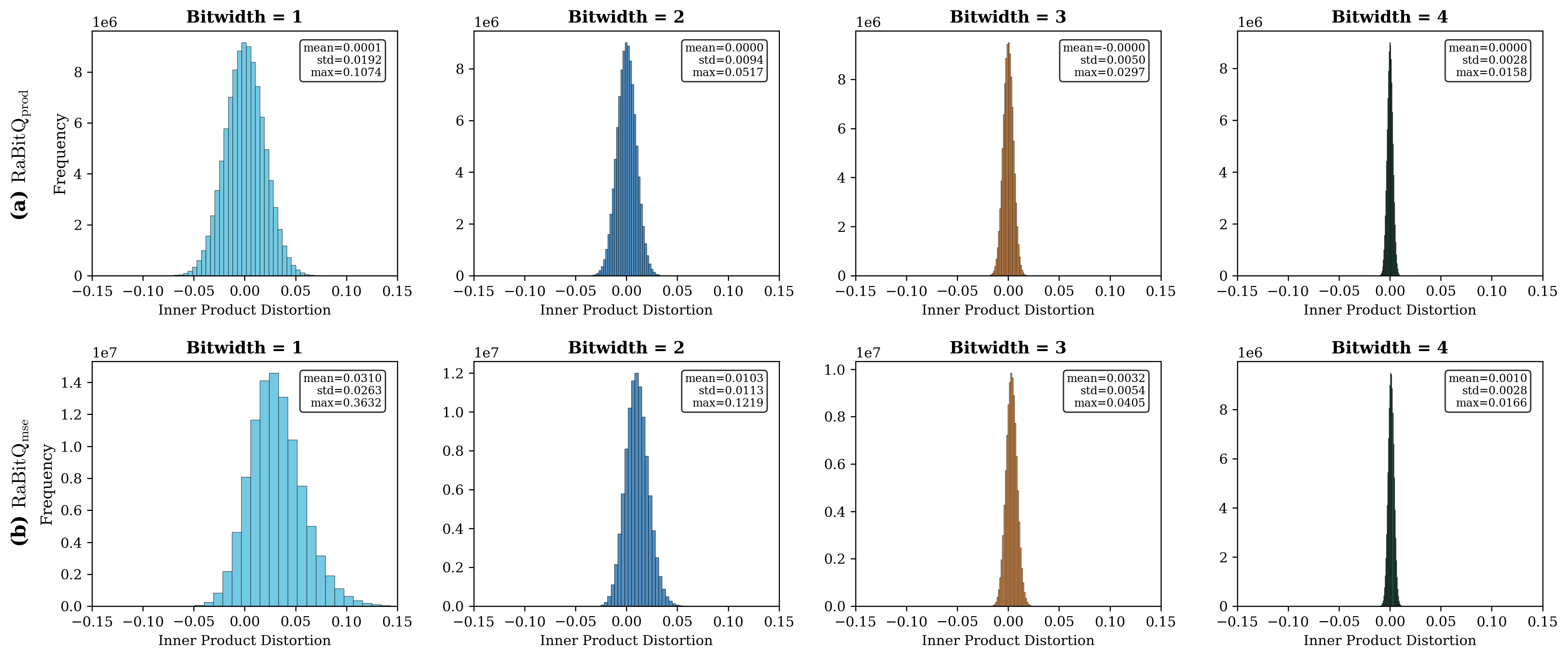
The image contains eight histograms arranged in a 2x4 grid, comparing the distribution of **Inner Product Distortion** across four bitwidths (1–4) for two metrics:
- **Top row (a)**: Frequency of RaBitQ_prod (y-axis: 0–1e6)
- **Bottom row (b)**: RaBitQ_mse (y-axis: 0–1e7)
Each subplot includes a legend with statistical summaries (mean, standard deviation, max) and uses distinct colors for clarity.
---
### Components/Axes
#### Labels and Titles
- **X-axis**: "Inner Product Distortion" (range: -0.15 to 0.15)
- **Y-axis (Top row)**: "Frequency" (log scale: 0–1e6)
- **Y-axis (Bottom row)**: "RaBitQ_mse" (log scale: 0–1e7)
- **Subplot Titles**: "Bitwidth = [1–4]"
- **Legend Labels**: "mean=[value]", "std=[value]", "max=[value]"
#### Color Coding
- **Top row (a)**: Blue histograms
- **Bottom row (b)**: Brown histograms (Bitwidth=1–3), Dark green (Bitwidth=4)
---
### Detailed Analysis
#### Top Row (RaBitQ_prod)
1. **Bitwidth=1**:
- **Mean**: 0.0001
- **Std**: 0.0192
- **Max**: 0.1074
- **Trend**: Broad, symmetric distribution centered near 0.
2. **Bitwidth=2**:
- **Mean**: 0.0000
- **Std**: 0.0094
- **Max**: 0.0517
- **Trend**: Narrower than Bitwidth=1, slightly left-skewed.
3. **Bitwidth=3**:
- **Mean**: -0.0000
- **Std**: 0.0270
- **Max**: 0.0297
- **Trend**: Sharp peak at 0, minimal spread.
4. **Bitwidth=4**:
- **Mean**: 0.0000
- **Std**: 0.0158
- **Max**: 0.0158
- **Trend**: Extremely narrow, near-perfect symmetry.
#### Bottom Row (RaBitQ_mse)
1. **Bitwidth=1**:
- **Mean**: 0.0310
- **Std**: 0.0263
- **Max**: 0.3632
- **Trend**: Broad distribution with a slight right skew.
2. **Bitwidth=2**:
- **Mean**: 0.0103
- **Std**: 0.0113
- **Max**: 0.1219
- **Trend**: Narrower than Bitwidth=1, centered near 0.
3. **Bitwidth=3**:
- **Mean**: 0.0032
- **Std**: 0.0054
- **Max**: 0.0405
- **Trend**: Sharp peak at 0, minimal spread.
4. **Bitwidth=4**:
- **Mean**: 0.0010
- **Std**: 0.0028
- **Max**: 0.0166
- **Trend**: Extremely narrow, near-perfect symmetry.
---
### Key Observations
1. **Bitwidth Correlation**:
- Higher bitwidths (3–4) show significantly narrower distributions, indicating reduced distortion.
- **RaBitQ_prod** and **RaBitQ_mse** both improve with increased bitwidth, but **RaBitQ_mse** values are consistently higher.
2. **Statistical Trends**:
- **Mean**: All distributions are centered near 0, with negligible bias.
- **Standard Deviation**: Decreases with bitwidth (e.g., Bitwidth=1: std=0.0192 → Bitwidth=4: std=0.0028).
- **Max Values**: Drop sharply with higher bitwidths (e.g., Bitwidth=1: max=0.1074 → Bitwidth=4: max=0.0158).
3. **Color Consistency**:
- Legends match histogram colors (e.g., Bitwidth=4 in dark green across both rows).
---
### Interpretation
The data demonstrates that **higher bitwidths improve precision** in inner product calculations:
- **RaBitQ_prod** and **RaBitQ_mse** both show reduced distortion as bitwidth increases, with Bitwidth=4 achieving near-zero mean and minimal spread.
- The **log-scale y-axes** highlight the exponential improvement in precision (e.g., RaBitQ_mse drops from ~0.36 to ~0.016 as bitwidth increases).
- The **narrowing histograms** visually confirm that higher bitwidths reduce variability, aligning with the statistical summaries.
This suggests that increasing bitwidth enhances computational accuracy, likely due to reduced quantization errors in fixed-point arithmetic.