# ArXiv Paper 0901.1705v1
## Rate-Distortion with Side-Information at Many Receivers
Roy Timo, Terence Chan and Alexander Grant
## Abstract
We present an inner bound for the admissible rate region of the t -stage successive refinement problem with side information, and we present an upper bound for the rate-distortion function for lossy source coding with multiple receivers and side information. A single-letter characterisation of this rate-distortion function is a long standing open problem in multi-terminal information theory, and it is widely believed that the tightest upper bound is provided by Theorem 2 of Heegard and Berger's paper 'Rate-Distortion when Side Information may be Absent,' IEEE Trans. Inform. Theory , 1985. We give a counterexample to Heegard and Berger's result, and we develop our new upper bound as a corollary to our inner bound for the successive refinement problem with side information.
## Index Terms
Source coding with receiver side information, rate-distortion function, successive refinement, complementary delivery, side information scalable source coding.
R. Timo, T. Chan and A. Grant are with the Institute for Telecommunications Research, University of South Australia. Email: { roy.timo, terence.chan, alex.grant } @unisa.edu.au. This work was funded by the Australian Research Council Grant DP0880223.
## I. INTRODUCTION
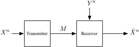
One of the most important results in multi-terminal information theory is Wyner and Ziv's solution [1] to the problem of lossy source coding with side information at the receiver; figure 1 shows the problem setup. The main objective is to give a single-letter characterisation [2, Page 259] of the rate-distortion function R ( d ) , which is defined as the smallest rate at which it is possible to encode a discrete memoryless source X n = X 1 , . . . , X n such that the receiver with side information Y n = Y 1 , . . . , Y n can obtain a reconstruction ˆ X n of X n with an average per-letter distortion less than d . To this end, Wyner and Ziv [1, Theorem 1] showed that
$$R ( d ) = \min \{ I ( X ; U ) - I ( U ; Y ) \}$$
where the minimization is over all choices of a discrete finite alphabet auxiliary random variable U such that: (1) Y /minuso X /minuso U forms a Markov chain, and (2) there exists a deterministic function ˆ X ( U, Y ) with an expected distortion less than d . In this paper we study two extensions of this problem with multiple receivers.
Fig. 1. Lossy source coding with side information at the receiver.
<details>
<summary>Image 1 Details</summary>
### Visual Description
## Block Diagram: Communication System Overview
### Overview
The image depicts a simplified block diagram of a communication system. It illustrates the flow of signals between a transmitter and a receiver, including the channel and signal transformations.
### Components/Axes
- **Components**:
- **Transmitter**: A rectangular block labeled "Transmitter" positioned on the left side of the diagram.
- **Receiver**: A rectangular block labeled "Receiver" positioned on the right side of the diagram.
- **Channel**: A horizontal arrow labeled "M" connecting the transmitter and receiver, representing the communication medium.
- **Signals**:
- **Input Signal**: Labeled $ X^n $, entering the transmitter from the left.
- **Output Signal**: Labeled $ Y^n $, exiting the receiver and pointing upward.
- **Estimated Signal**: Labeled $ \hat{X}^n $, exiting the receiver and pointing to the right.
### Detailed Analysis
- **Signal Flow**:
1. The input signal $ X^n $ is processed by the transmitter.
2. The processed signal travels through the channel $ M $ to the receiver.
3. The receiver processes the signal, producing two outputs:
- $ Y^n $, which is transmitted upward (possibly representing feedback or a secondary output).
- $ \hat{X}^n $, the estimated version of the original input signal $ X^n $, transmitted to the right.
### Key Observations
- The diagram emphasizes the bidirectional relationship between the transmitter and receiver, with the channel $ M $ acting as a mediator.
- The use of $ \hat{X}^n $ suggests the receiver performs estimation or reconstruction of the original signal, potentially accounting for noise or distortion in $ M $.
- No numerical values or quantitative data are present; the diagram focuses on structural relationships.
### Interpretation
This diagram represents a foundational model of a communication system, highlighting the roles of the transmitter, receiver, and channel. The inclusion of $ \hat{X}^n $ implies that the receiver employs algorithms (e.g., filtering, decoding) to recover the original signal from the received $ Y^n $. The upward arrow for $ Y^n $ may indicate a feedback loop or a separate output for monitoring purposes. The absence of explicit noise or error terms suggests an idealized scenario, though real-world implementations would likely include such factors. The diagram underscores the importance of signal processing in ensuring accurate transmission and reception.
</details>
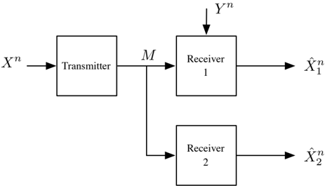
If the side information Y n in Wyner and Ziv's problem becomes unreliable in the sense that it may, or may not, be available to the receiver, then the coding scheme [1, Section IV] used to prove (1) fails: a more complex coding scheme is required to exploit Y n . This observation independently inspired Kaspi [3] in 1980 (published by Wyner on behalf of Kaspi in 1994) as well as Heegard and Berger [4] in 1985 to consider problem shown in Figure 2 - the so called Kaspi/Heegard-Berger problem. As before, the objective is to find the smallest rate R ( d 1 , d 2 ) such that receiver 1 resp. 2 can find reconstructions with average per-letter distortions d 1 resp. d 2 . Heegard and Berger 1 showed that [4, Theorem 1]
$$R ( d _ { 1 } , d _ { 2 } ) = \min \{ I ( X ; U | Y, W ) ,$$
1 Kaspi's result [3, Theorem 2] gives an alternative characterisation of R ( d 1 , d 2 ) .
where the minimization is over all choices of two discrete finite alphabet auxiliary random variables U and W such that: (1) Y /minuso X /minuso ( U, W ) forms a Markov chain, and (2) there exists functions ˆ X 1 ( Y, U, W ) and ˆ X 2 ( W ) with expected distortions bound by d 1 and d 2 respectively.
Fig. 2. Lossy source coding when side information may be absent at the receiver.
<details>
<summary>Image 2 Details</summary>
### Visual Description
## Block Diagram: Communication System with Two Receivers
### Overview
The diagram illustrates a communication system where a transmitter sends a signal \( X^n \) through a channel \( M \) to two receivers. Each receiver processes the signal and outputs an estimated version (\( \hat{X}_1^n \) and \( \hat{X}_2^n \)). The system includes variables \( X^n \), \( Y^n \), and channel \( M \), with directional flow indicated by arrows.
### Components/Axes
- **Transmitter**: Receives input \( X^n \) and transmits it through channel \( M \).
- **Channel \( M \)**: Represents the medium or process through which the signal propagates.
- **Receiver 1**: Processes the transmitted signal and outputs \( \hat{X}_1^n \).
- **Receiver 2**: Processes the transmitted signal and outputs \( \hat{X}_2^n \).
- **Variables**:
- \( X^n \): Input signal to the transmitter.
- \( Y^n \): Output signal from the channel (not directly connected to receivers in this diagram).
- \( \hat{X}_1^n \), \( \hat{X}_2^n \): Estimated signals from Receivers 1 and 2, respectively.
### Detailed Analysis
- **Flow Direction**:
- \( X^n \) → Transmitter → Channel \( M \) → Receiver 1 → \( \hat{X}_1^n \).
- \( X^n \) → Transmitter → Channel \( M \) → Receiver 2 → \( \hat{X}_2^n \).
- **Key Variables**:
- \( X^n \): Original transmitted signal.
- \( Y^n \): Channel output (not explicitly linked to receivers in this diagram).
- \( \hat{X}_1^n \), \( \hat{X}_2^n \): Estimated signals at each receiver.
- **Channel \( M \)**: Acts as a shared medium for both receivers, suggesting potential interference or collaborative processing.
### Key Observations
1. **Parallel Processing**: Both receivers operate independently on the same transmitted signal \( X^n \), implying redundancy or diversity in signal estimation.
2. **Estimation Focus**: The system emphasizes reconstructing the original signal (\( \hat{X}_1^n \), \( \hat{X}_2^n \)) from the channel output \( M \).
3. **No Direct Feedback**: There is no explicit feedback loop from receivers to the transmitter or channel.
### Interpretation
This diagram represents a **multiple-access or broadcast channel** scenario where a single transmitter communicates with multiple receivers. The use of \( \hat{X}_1^n \) and \( \hat{X}_2^n \) suggests the receivers perform **signal estimation** or **decoding** tasks, possibly in the presence of noise or interference (implied by channel \( M \)). The absence of \( Y^n \) in the receiver outputs indicates \( Y^n \) may represent an intermediate or unobserved state in the channel.
The system could model applications like **wireless communication**, **sensor networks**, or **distributed computing**, where reliable signal recovery across multiple receivers is critical. The lack of explicit error-correction mechanisms or feedback loops implies the focus is on open-loop estimation rather than iterative refinement.
</details>
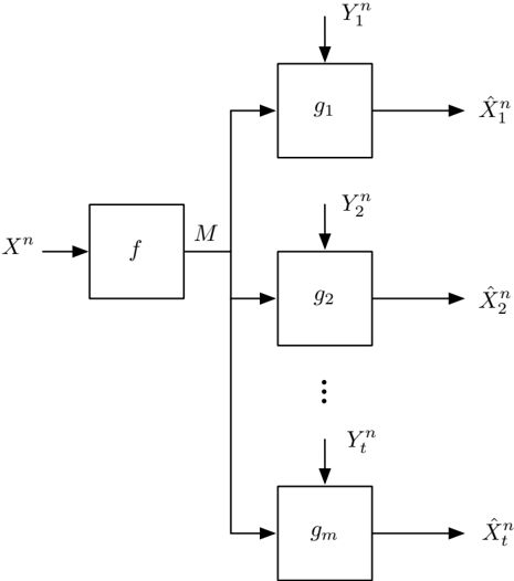
The Kaspi/Heegard-Berger problem was further generalised by Heegard and Berger in [4, Section VII] to the problem shown in Figure 3. There are t receivers (each with their own side information) and the objective is to characterise the corresponding rate-distortion function R ( d 1 , d 2 , . . . , d t ) . Today, a single-letter characterisation of R ( d 1 , d 2 , . . . , d t ) is still lacking; since its formulation in 1985, Heegard and Berger's problem has resisted final solution and is now regarded as a classic in multi-terminal information theory. Notwithstanding this difficulty, the problem has stimulated a number of important results over the past two decades [3], [5]-[9], and it has been solved for the special case of degraded side information X /minuso Y { t } /minuso Y { t -1 } /minuso · · · /minuso Y { 1 } [4, Theorem 3].
For arbitrarily correlated side information, Heegard and Berger presented the function R HB ( d 1 , d 2 , . . . , d t ) in [4, Theorem 2] as an upper bound for R ( d 1 , d 2 , . . . , d t ) . (The expression for R HB ( d 1 , d 2 , . . . , d t ) follows in (14); however, this expression requires the notation and definitions from Section II.) This function is widely believed to be the tightest upper bound.
The present paper was motivated by our discovery of a counterexample to [4, Theorem 2]. That is, a situation where the claimed upper bound R HB ( d 1 , d 2 , . . . , d t ) is strictly less than the rate distortion function R ( d 1 , d 2 , . . . , d t ) . The invalidity of R HB ( d 1 , d 2 , . . . , d t ) as an upper bound for R ( d 1 , d 2 , . . . , d t ) is by no means obvious. Despite being used with modest frequency in the literature, it appears to have gone unnoticed for more than two decades. The claim is based on a complex random coding argument that uses 2 t -1 individual descriptions (via 2 t -1 auxiliary random variables) to convey information
about X n to the receivers. We will see, however, that the expression for R HB ( d 1 , d 2 , . . . , d t ) does not provide appropriate conditional independence between certain auxiliary random variables; thus, there is insufficient rate for each of the 2 t -1 descriptions to be reliably decoded at the receivers.
Fig. 3. Lossy source coding with t receivers - each with arbitrary side information.
<details>
<summary>Image 3 Details</summary>
### Visual Description
## Flowchart Diagram: Multi-Stage Processing System
### Overview
The diagram illustrates a multi-stage processing system with sequential and parallel components. Input data `X^n` flows through a function `f`, then a module `M`, which distributes the data to multiple processing blocks (`g1` to `gm`). Each block produces an output `X̂_i^n` (where `i` ranges from 1 to `m`), with intermediate inputs `Y^n` feeding into subsequent blocks.
### Components/Axes
- **Input**: `X^n` (initial data input)
- **Function**: `f` (transforms `X^n` before processing by `M`)
- **Module**: `M` (distributes processed data to parallel blocks)
- **Processing Blocks**:
- `g1` to `gm` (each processes `Y^n` and outputs `X̂_i^n`)
- **Intermediate Inputs**: `Y^n` (inputs to each `g_i` block)
- **Outputs**: `X̂_1^n` to `X̂_t^n` (transformed outputs from each block)
### Detailed Analysis
- **Flow Structure**:
1. `X^n` → `f` → `M` (sequential processing).
2. `M` branches into `m` parallel paths (`g1` to `gm`).
3. Each `g_i` takes `Y^n` as input and produces `X̂_i^n`.
- **Notation**:
- `Y^n` appears as both an output from `M` and an input to all `g_i` blocks, suggesting it is a shared intermediate variable.
- `X̂_i^n` denotes the output of the `i`-th block, with `i` ranging from 1 to `m` (exact value of `m` unspecified).
- **Spatial Layout**:
- Vertical flow from top (`X^n`) to bottom (`X̂_t^n`).
- `M` is centrally positioned, with `g1` to `gm` arranged horizontally below it.
### Key Observations
- The system combines **sequential** (`f`, `M`) and **parallel** (`g1` to `gm`) processing.
- The use of `Y^n` as a shared input to all `g_i` blocks implies a common intermediate representation or feature extraction step.
- The diagram does not specify the exact number of blocks (`m`) or the nature of transformations (`f`, `g_i`).
### Interpretation
This diagram represents a **modular architecture** for data processing, likely designed for tasks requiring parallel computation (e.g., machine learning pipelines, signal processing). The module `M` acts as a **distribution hub**, enabling scalability by splitting workloads across multiple blocks. The shared `Y^n` suggests a **feature extraction** or **normalization** step before parallel processing. The absence of numerical data or explicit trends indicates the focus is on **system design** rather than performance metrics. The use of `X̂_i^n` implies outputs are transformed versions of inputs, potentially for tasks like prediction, classification, or reconstruction.
</details>
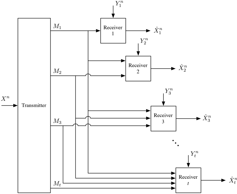
This observation led us to consider the generalisation of Heegard and Berger's problem shown in Figure 4. The transmitter encodes the source into t messages M 1 , M 2 , . . . , M t . Receiver j receives messages M 1 through M j and forms a reconstruction ˆ X j with average per-letter distortion less than d j . It is readily seen that this generalisation of Heegard and Berger's problem is a multi-stage version of the successive refinement problem with side information [6], [8], [9], and for this reason we refer to it as a successive refinement problem 2 .
Steinberg and Merhav [6] introduced and solved the two-receiver successive refinement problem with degraded side information X /minuso Y 2 /minuso Y 1 , and Tian and Diggavi [9] extended this solution to t -receivers
2 In this paper we shall be exclusively interested in the characterisation of an inner bound for the region of admissible rate tuples. We will not require, or even define, any notion of successive refinability of the source. For such details, the interested reader is directed to [6], [8], [9].
with degraded side information X /minuso Y t /minuso · · · /minuso Y 2 /minuso Y 1 . More recently, Tian and Diggavi [8] gave inner and outer bounds for the admissible rate region for two receivers assuming X /minuso Y 1 /minuso Y 2 forms a Markov chain - a reverse of the degradedness X /minuso Y 2 /minuso Y 1 used in [6], [9]. Our main result is a coding theorem for the t -stage successive refinement problem with arbitrarily correlated side information shown in Figure 4. An immediate corollary of this theorem is an upper bound for the rate-distortion function R ( d 1 , d 2 , . . . , d t ) for Heegard and Berger's problem shown in Figure 3.
n
Fig. 4. Successive Refinement with t stages and side information.
<details>
<summary>Image 4 Details</summary>
### Visual Description
## Block Diagram: Communication System Architecture
### Overview
The diagram illustrates a multi-receiver communication system where a single transmitter sends messages to multiple receivers. Each receiver processes its input signal to estimate the original transmitted message. The system includes parallel processing paths for scalability.
### Components/Axes
- **Transmitter**: Central block on the left, labeled with sequential messages `M₁, M₂, ..., Mₜ`.
- **Receivers**: Labeled `Receiver 1` to `Receiver t`, arranged vertically on the right.
- **Signals**:
- Input signals: `Y₁ⁿ, Y₂ⁿ, ..., Yₜⁿ` (received at each receiver).
- Output estimates: `X̂₁ⁿ, X̂₂ⁿ, ..., X̂ₜⁿ` (estimated messages from each receiver).
- **Flow Direction**: Arrows indicate data flow from the transmitter to receivers and from receiver inputs to outputs.
### Detailed Analysis
- **Transmitter**:
- Generates messages `M₁` to `Mₜ`, which are distributed to all receivers.
- Messages are not explicitly labeled as transmitted signals but are implied as inputs to the receivers.
- **Receivers**:
- Each receiver `i` processes its input `Yᵢⁿ` to produce an estimated message `X̂ᵢⁿ`.
- Receivers operate independently, with no feedback loops shown.
- **Signals**:
- `Yᵢⁿ` (input to receiver `i`) and `X̂ᵢⁿ` (output from receiver `i`) are linked by arrows, suggesting a transformation or estimation process.
- No explicit noise or channel models are depicted.
### Key Observations
- The system scales linearly with the number of receivers (`t`), as each receiver has a dedicated processing path.
- No explicit error correction or feedback mechanisms are shown, implying a one-way communication model.
- The use of `n` in `Yᵢⁿ` and `X̂ᵢⁿ` suggests time-indexed or sample-specific signals (e.g., `n`-th time step).
### Interpretation
This diagram represents a **parallel distributed receiver architecture** for message recovery. The transmitter broadcasts messages to all receivers, which independently process their received signals (`Yᵢⁿ`) to estimate the original message (`X̂ᵢⁿ`). The absence of feedback or error-handling components suggests a focus on simplicity or real-time processing. The system could model scenarios like:
- **Broadcast Communication**: A single source (e.g., a satellite) transmitting data to multiple ground stations.
- **Sensor Networks**: A central node sending commands to distributed sensors, each estimating local states.
- **Machine Learning**: A central model generating inputs for multiple parallel inference engines.
The diagram emphasizes scalability (`t` receivers) and modularity, with each receiver functioning as an independent estimator. The lack of explicit channel noise or synchronization mechanisms implies idealized conditions or assumptions of perfect transmission.
</details>
An outline of the remainder of this paper is as follows. In Section II we formally define the t -receiver successive refinement problem shown in Figure 4; we present an inner bound for the admissible rate region in Theorem 1; and we show that this inner bound includes the coding theorems of Steinberg and Merhav [6] as well as Tian and Diggavi [8], [9] as special cases. Our proof of Theorem 1 is given in Section III. In Section IV we formally define Heegard and Berger's problem shown in Figure 3; we show
that there exists a situation where R HB ( d 1 , d 2 , . . . , d t ) < R ( d 1 , d 2 , . . . , d t ) ; we present a new upper bound for R ( d 1 , d 2 , . . . , d t ) in Corollary 1; and we show that this bound includes the coding theorems of Wyner and Ziv [1], Heegard and Berger [4], and Kimura and Uyematsu [10] as a special case. In Section V we describe a new lossless source coding problem and present an achievable rate. Finally, the paper is concluded in Section VI.
Notation: Sets will be identified using calligraphic typeface, e.g. X ; random variables will be identified by upper case characters 3 e.g. X ∈ X ; and particular realizations of random variables will be identified by lowercase characters e.g. x . Superscripts will be used to denote sequences, e.g. X j = X 1 , X 2 , . . . , X j , similarly X j i = X i , X i +1 , . . . , X j . For any natural number t ∈ N we let [ t ] = { 1 , 2 , . . . , t } , and for s < t we let [ s, t ] = { s, s +1 , . . . , t } . Set-valued subscripts will serve as indices 4 , e.g. U S with S ⊂ [ t ] denotes the random variable assigned to the subset S . For brevity, singletons or other small sets will be written without brace notation, e.g. U { 1 } and U { 1 , 2 } will be written as U 1 and U 12 respectively. Sequences of so-labelled variables will be denoted by U j S ,i = U S ,i , U S ,i +1 , . . . , U S ,j . Finally, tuples will be denoted by boldface, e.g. d = ( d 1 , d 2 , . . . , d t ) .
## II. SUCCESSIVE REFINEMENT WITH RECEIVER SIDE INFORMATION
We begin with a formal definition of the problem that is shown in Figure 4. Let X and Y j (for all receivers j ∈ [ t ] ) be discrete finite alphabets. We assume that
$$( X _ { i } , Y _ { 1 } , Y _ { 2 } , \ldots , Y _ { t } ) \Delta \{ ( X _ { i } , Y _ { 1 } , Y _ { 2 } , \ldots , Y _ { t } ) \} ^ { n } = 1$$
are n independent and identically distributed (i.i.d.) tuples of random variables emitted by a discrete memoryless source ( X × Y 1 × Y 2 × · · · × Y t , Q ) , where Q is an arbitrary probability mass function on the cartesian product space X × Y 1 × Y 2 × · · · × Y t :
$$x _ { 1 } , y _ { 1 } = y _ { 1 } , \ldots , y _ { t } = y _ { t } .$$
The transmitter encodes X n with an encoder
$$f ^ { \prime } ( n ) : x ^ { n } - M _ { 1 }$$
where M j is a discrete finite set with | M j | elements. The resulting t indices ( M 1 , M 2 , . . . , M t ) = f ( n ) ( X n ) are sent to the receivers over channels 1 through t respectively.
3 With the exception of H and I , which will be respectively reserved for the entropy and mutual information functions as defined in [11]. Similarly, R will be reserved for rate-distortion functions and admissible rates.
4 Rather than to denote the set { U i , i ∈ S } of random variables, which is common usage in the literature.
At the j th -receiver, let ˆ X j be a reconstruction alphabet and δ j : X × ˆ X j → R + /defines [0 , ∞ ) be a per-letter distortion measure. (The reconstruction alphabet and distortion measure used at each receiver need not be identical.) The j th -receiver is required to generate a reconstruction ˆ X n j = g ( n ) j ( M 1 ,M 2 , . . . , M j , Y n j ) of X n using a decoder
$$g ^ { ( n ) } : M _ { 1 } \times M _ { 2 } \times \cdots$$
and the quality of this reconstruction is measured by the average distortion
$$\Delta _ { j } = - \sum _ { i = 1 } ^ { n } \delta _ { j ( X _ { i } , X _ { j } ) }$$
where E denotes the expectation operator.
Definition 1 ( d -Admissible Rate Tuple): Suppose d = ( d 1 , d 2 , . . . , d t ) ∈ R t + is an arbitrary distortion tuple. A rate tuple R = ( R 1 , R 2 , . . . , R t ) ∈ R t + is said to be d -admissible if, for arbitrary /epsilon1 > 0 , there exists a sufficiently large n , an encoder f ( n ) and t decoders g ( n ) 1 , g ( n ) 2 , . . . , g ( n ) t , where ∆ j ≤ d j + /epsilon1 and
$$\frac { 1 } { n } - \log _ { 2 } | M _ { j } | \leq R _ { j } + c$$
for every j ∈ [ t ] . We let R ( d ) denote the closure of the set of all d -admissible rate tuples.
For each j ∈ [ t ] , let d j,min = E [min ˆ x ∈ ˆ X j δ j ( X, ˆ x )] . If d j < d j,min for any receiver j ∈ [ t ] , then there is no rate tuple R ∈ R t + for which the distortion tuple d is admissible; the set R ( d ) is empty. In the following, we are interested in the characterisation of R ( d ) for distortion tuples where d j ≥ d j,min for all j ∈ [ t ] . The following proposition shows that this region is always convex; its proof follows from the standard code time sharing argument [12, Appedix].
Proposition 1: If d ∈ R t + with d j ≥ d j,min for all j ∈ [ j ] , then the d -admissible rate region R ( d ) is a closed convex subset of R t + .
The inner bound that we will develop in Theorem 1 requires 2 t -1 auxiliary random variables - one for each non-empty subset of receivers. For this purpose we let, for each non-empty subset S ⊆ [ t ] , AS be a discrete finite alphabet and U S be an auxiliary random variable defined on AS . Additionally, we let U /defines { U T ; ∅ /negationslash = T ⊆ [ t ] } be the set of all such auxiliary variables, and we define the following two subsets of U :
/negationslash
$$u ^ { \ast } ( p ) \Delta \{ U _ { g } : g \in \Gamma \} = \{ u _ { 1 } ( p ) \}, and$$
/negationslash
We define the auxiliary random variables in U via a family of probability mass functions P ( d , Q ) on ∏ S AS × X × Y 1 ×··· × Y t . Specifically, a probability mass function p is a member of P ( d , Q ) if it satisfies the following four properties:
- (P1) The X × Y 1 × Y 2 ×··· × Y t marginal of p is equal to Q .
- (P2) p factors to form the Markov chain U /minuso X /minuso ( Y 1 , Y 2 , . . . , Y t ) .
- (P3) For every subset S ⊆ [ t ] , p factors to form the Markov chain U S /minuso ( U ∗ ( S ) , X ) /minuso U † ( S ) .
- (P4) For every receiver j ∈ [ t ] , there exists a deterministic function ˆ X j ( Y j , U j , U ∗ ( j )) with
$$E _ { j } ( X , \hat { X } , U , g ^ { r } ( i ) ) \leq d .$$
For each mass function p ∈ P ( d , Q ) , define
$$\sum _ { i = 1 } ^ { n } \sum _ { j = 1 } ^ { m } R _ { i , j } \geq \sum _ { i = 1 } ^ { n } \sum _ { j = 1 } ^ { m } I ( X ; U _ { g } | Y _ { i } , \varphi * ) = 1$$
and let
$$\sum _ { i = 1 } ^ { j } R _ { i } \geq \sum _ { i \in S ( n | j ) } I ( X ; U _ { g } | Y _ { i } , w )$$
where co ( · ) denotes the closure of the convex hull. The following theorem is the main result of the paper.
/negationslash
$$\rho ^ { \ast } ( d ) = c 0 \{ U \rho _ { \alpha } ( d , p ) \} ,$$
Theorem 1: If d ∈ R t + and d j ≥ d j, min for every receiver j ∈ [ t ] , then every rate tuple within R ∗ ( d ) is d -admissible:
$$R ^ { \prime } ( d ) = R ( d ) .$$
The proof of this coding theorem is provided in the next section. The following two examples show that this inner bound yields the entire d -admissible rate region when the side information is degraded, and it reduces to the largest known inner bound for the side information scalable source coding problem.
/negationslash
Example 1 (Degraded Side Information): The side information is said to be degraded if X /minuso Y t /minuso Y t -1 /minuso · · · /minuso Y 1 forms a Markov chain. The first result for degraded side information was provided by Steinberg and Merhav [6, Theorem 1] for two receivers t = 2 . This result was subsequently extended by Tian and Diggavi [9, Theorem 1] to any finite number of receivers t > 2 . To see how Theorem 1 gives the coding part of [9, Theorem 1] consider the following. Suppose d ∈ R t + with d j ≥ d j,min for all j ∈ [ t ] , and let P deg ( d , Q ) denote those mass functions in P ( d , Q ) where U S is degenerate (constant) whenever S = [ j, t ] for some j ∈ [ t ] . For each p ∈ P deg ( d , Q ) , the region specified by (2) simplifies to
$$\sum _ { i = 1 } ^ { j } \sum _ { i = 1 } ^ { j } I ( X ; U _ { i , j } ) | Y _ { i } ; U _ { 1 , t } ; U _ { 2 , t } )$$
which is the desired result.
Example 2 (Side Information Scalable Source Coding): When t = 2 and X /minuso Y 2 /minuso Y 1 forms a Markov chain, Heegard and Berger [4, Theorem 3] showed that an optimal compression strategy should satisfy distortion constraints of receiver 2 after the distortion constraints of receiver 1 have been satisfied. However, if the side information is not degraded, then this ordering may not be optimal. This observation lead Tian and Diggavi [8] to propose the side information scalable source coding problem, where it is assumed that X /minuso Y 1 /minuso Y 2 forms a Markov chain. Under this Markov constraint, the region defined by (2) reduces to
$$\begin{array}{ll}
\varphi ( d , p ) = \left\{ \begin{matrix} R _ { 1 } : R _ { 2 } \in R ^ { 4 } : R _ { 1 } + R _ { 2 } \geq I ( X ; U _ { 1 } , U _ { 2 } | Y _ { 1 } ) \\ + I ( X ; U _ { 1 } | Y _ { 1 } , U _ { 2 } ) \end{matrix} \right.
\end{array}$$
which yields the inner bound reported in [8, Theorem 1]. A single-letter solution for this problem remains open.
## III. PROOF OF THEOREM 1
We now show that every rate tuple R ∈ R ( d , p ) is d -admissible for any p ∈ P ( d , Q ) . (The d -admissibility of rate tuples in R ∗ ( d ) follows by the standard code time sharing argument.) The main ingredient of the proof is a multi-layered random coding argument, which uses Kramer's notion of /epsilon1 -letter typical sequences [13]. For convenience, we have reviewed the relevant /epsilon1 -letter typical results in Appendix II. Finally, to help elucidate the main ideas of the random coding argument, we present the special case of t = 3 receivers as a series of examples in parallel to the main proof.
## A. Code Construction
Suppose d ∈ R t + (with d j ≥ d j,min for every receiver j ∈ [ t ] ) and p ∈ P ( d , Q ) are given. For each non-empty subset S ⊆ [ t ] , construct an | S | -layer nested codebook in the following manner: for each vector valued index
$$k _ { y } = ( k _ { y } , k _ { y } 2 , \ldots , k _ { y } | g | , k _ { y } ) ,$$
with k S ,i ∈ [2 nR S ,i ] , i = 1 , 2 , . . . , | S | and k ′ S ∈ [2 nR ′ S ] , generate a length n codeword a n S ( k S ) ∈ A n S by selecting n symbols from AS in an i.i.d. manner using the U S marginal of p . The quantities R S ,i and R ′ S will be defined shortly.
Example 3 ( 3 -Receivers Code Construction): We construct seven nested codebooks; one codebook for each non-empty subset of { 1 , 2 , 3 } . Figure 5 shows the 3 -layer nested codebook associated with the subset
{ 1 , 2 , 3 } . In the first layer, there are 2 nR 123 , 1 bins (labelled with the index k 123 , 1 ) each of which contain 2 n ( R ′ 123 + R 123 , 2 + R 123 , 3 ) codewords. The set of codewords inside a particular layer one bin define the second layer of the codebook. Specifically, each layer one index k 123 , 1 ∈ [2 nR 123 , 1 ] identifies 2 nR 123 , 2 layer two bins. These bins are labelled with the index k 123 , 2 , and each bin contains 2 n ( R ′ 123 + R 123 , 3 ) codewords. Similarly, each pair k 123 , 1 ∈ [2 nR 123 , 1 ] and k 123 , 2 ∈ [2 nR 123 , 2 ] identifies 2 nR 123 , 3 layer three bins. There are 2 n ( R ′ 123 ) codewords in each one of the layer three bins.
Fig. 5. Three-layer codebook.
<details>
<summary>Image 5 Details</summary>

### Visual Description
## Diagram: Hierarchical Codeword Binning Structure
### Overview
The diagram illustrates a hierarchical organization of codewords into bins with decreasing granularity. A central flow of "2^nR'_S codewords" descends into multiple nested sections, each labeled with progressively smaller bin counts (e.g., "2^nR'_S,3 bins", "2^nR'_S,2 bins", "2^nR'_S,1 bins"). Arrows indicate directional flow from codewords to bins, with visual segmentation into distinct regions.
### Components/Axes
- **Main Title**: "2^nR'_S codewords" (top-left, bold, arrowed)
- **Regions**:
- **Top Section**: Labeled "2^nR'_S,3 bins" (leftmost, 3 vertical rectangles per bin)
- **Middle Sections**: Labeled "2^nR'_S,2 bins" (center, 2 vertical rectangles per bin)
- **Bottom Section**: Labeled "2^nR'_S,1 bins" (rightmost, 1 vertical rectangle per bin)
- **Visual Elements**:
- Rectangular bins with vertical lines (single or double) inside
- Dotted lines separating regions
- Arrows pointing downward from codewords to bins
### Detailed Analysis
- **Codeword Flow**: The "2^nR'_S codewords" originate at the top and distribute into bins below. The number of bins decreases as the exponent in the label reduces (3 → 2 → 1).
- **Bin Structure**:
- **2^nR'_S,3 bins**: Each bin contains 3 vertical rectangles (possibly sub-bins or data units).
- **2^nR'_S,2 bins**: Each bin contains 2 vertical rectangles.
- **2^nR'_S,1 bins**: Each bin contains 1 vertical rectangle.
- **Spatial Grounding**:
- Labels are positioned above their respective regions.
- Arrows originate from the top-left codeword label and point to all bins.
- Dotted lines separate regions horizontally.
### Key Observations
- **Hierarchical Segmentation**: Bins are organized in tiers, with higher exponents (e.g., 3) representing coarser divisions and lower exponents (e.g., 1) finer divisions.
- **Consistent Flow**: All codewords funnel into bins regardless of bin size, suggesting uniform processing across tiers.
- **Visual Symmetry**: Bin regions are evenly spaced, with identical structural patterns (rectangles with vertical lines).
### Interpretation
The diagram likely represents a multi-stage encoding or error-correction process where codewords are partitioned into bins of varying granularity. The decreasing bin counts (3 → 2 → 1) may correspond to error-correction levels, with larger bins (higher exponents) handling broader error ranges and smaller bins (lower exponents) addressing finer details. The uniform flow of codewords into all bins suggests a cascading error-correction mechanism, where each tier refines the data further. The absence of numerical values implies the diagram abstracts the conceptual structure rather than specific quantitative data.
</details>
## B. Encoding
To describe the encoding and decoding procedure, it will be convenient to introduce some additional notation. Arrange the subsets of [ t ] into a list with descending cardinality. (For subsets with the same cardinality, use lexicographical ordering). With a slight abuse of notation, label the resulting list with the sequence S 1 , S 2 , . . . , S 2 t -1 . For example, for t = 3 receivers we have: S 1 = { 1 , 2 , 3 } , S 2 = { 1 , 2 } , S 3 = { 1 , 3 } , S 4 = { 2 , 3 } , S 5 = { 1 } , S 6 = { 2 } and S 7 = { 3 } . Now define
/negationslash
$$u + ( g _ { i } ) \Delta u _ { i } : A _ { i } n s$$
to be those auxiliary random variables labelled by lower indexed sets, which share at least one element with S j and have the same size as S j . Finally, let S ( i ) denote the i -th element of S under natural ordering. For example, if S = { 1 , 3 } then S (1) = 1 and S (2) = 3 .
Encoding proceeds sequentially in 2 t -1 stages using /epsilon1 -letter typical set encoding rules. For this purpose, choose 0 < /epsilon1 0 < /epsilon1 1 < · · · < /epsilon1 2 t to be arbitrarily small real numbers.
The transmitter is given a vector x n ∈ X n . At encoding stage j (for j = 1 , 2 , . . . , 2 t -1 ), it selects the codebook with label S j and looks for an index vector k S j where the corresponding codeword a n S j ( k S j )
Fig. 6. The figure illustrates the label and channel-to-index assignments for three receivers.
| S j | Subset | A.R.V. | U ‡ ( S j ) | Index-to-Channel Map |
|-------|---------------|----------|------------------|-------------------------------------------------------------------|
| S 1 | { 1 , 2 , 3 } | U S 1 | ∅ | k S 1 , 1 → Channel 1 k S 1 , 2 → Channel 2 k S 1 , 3 → Channel 3 |
| S 2 | { 1 , 2 } | U S 2 | ∅ | k S 2 , 1 → Channel 1 k S 2 , 2 → Channel 2 |
| S 3 | { 1 , 3 } | U S 3 | ˘ U S 2 ¯ | k S 3 , 1 → Channel 1 k S 3 , 2 → Channel 3 |
| S 4 | { 2 , 3 } | U S 4 | ˘ U S 2 ,U S 3 ¯ | k S 4 , 1 → Channel 2 k S 4 , 2 → Channel 3 |
| S 5 | { 1 } | U S 5 | ∅ | k S 5 , 1 → Channel 1 |
| S 6 | { 2 } | U S 6 | ∅ | k S 6 , 1 → Channel 2 |
| S 7 | { 3 } | U S 7 | ∅ | k S 7 , 1 → Channel 3 |
is /epsilon1 j -letter typical with x n ,
/negationslash
If successful 5 , the transmitter sends the bin index k S j ,i over channel S j ( i ) for each i = 1 , 2 , . . . , | S j | . If unsuccessful, the transmitter sends k S j ,i = 1 over each of these channels.
$$\begin{aligned}
\{ \alpha ^ { n } _ { i } ( k _ { p } ) : \gamma _ { i } \geq 1 , i < j \}, and \\
i \neq 0, | \gamma _ { i } | = | \gamma _ { j } |, i < j . \\
\end{aligned}$$
Example 4 ( 3 -Receivers Encoding): Figure 6 illustrates the labels used to identify the seven non-empty subsets of { 1 , 2 , 3 } ; the assignment of seven auxiliary random variables; the members of each of the sets U ‡ ( S j ) ; and the channels on which the bin indices are sent. In the first encoding stage, the transmitter looks for a vector k S 1 = ( k S 1 , 1 , k S 1 , 2 , k S 1 , 3 , k ′ S 1 ) such that the corresponding codeword a n S 1 ( k S 1 ) is typical with x n . The indices k S 1 , 1 , k S 1 , 2 and k S 1 , 3 are sent over channels 1 , 2 and 3 respectively. In the fourth encoding stage, the encoder looks for a vector k S 4 = ( k S 4 , 1 , k S 4 , 2 , k ′ S 4 ) such that the corresponding codeword a n S 4 ( k S 4 ) is typical with a n S 1 ( k S 1 ) , a n S 2 ( k S 2 ) , a n S 3 ( k S 3 ) and x n . Similarly, in the sixth encoding stage, the transmitter looks for a vector k S 6 = ( k S 6 , 1 , k ′ S 6 ) such that the corresponding codeword a n S 6 ( k S 6 ) is typical with a n S 1 ( k S 1 ) , a n S 2 ( k S 2 ) , a n S 4 ( k S 4 ) and x n .
5 If there are two-or-more such codewords, we assume that the transmitter selects one codeword arbitrarily and sends the corresponding indices.
## C. Decoding
Like the encoding procedure, receiver l (for each l ∈ [ t ] ) forms its reconstruction ˆ X n l using 2 t -1 sequential decoding stages. Recall, receiver l recovers every bin index transmitted on channels 1 through l ; it does not have access to any index transmitted on channels l +1 through t . In stage j (for all stages j = 1 , 2 , . . . , 2 t -1 ) it considers subset S j . If l / ∈ S j , then it does nothing and moves to decoding stage j +1 . If l ∈ S j , then it takes the bin indices
$$\{ k _ { z } , i = 1 , 2 , \ldots , \vert \vert 0 \vert \vert g \vert \}$$
and looks for an index vector ˜ k S j , with ˜ k S j ,i = k S j ,i for all i = 1 , 2 , . . . , | [ l ] ∩ S j | , such that the corresponding codeword a n ( ˜ k S j ) is /epsilon1 j +1 -letter typical with y n l and those codewords which belong to supersets of S j :
There are exactly
$$( { \alpha _ { i } ( k , j ) : x _ { i } \geq 2 } , ( 4 )$$
$$\sum _ { i = 1 } ^ { n } R _ { g , i }$$
codewords in the bin specified by the indices { k S j ,i : i = 1 , 2 , . . . , | [ l ] ∩ S j |} . If one or more of these codewords satisfy this typicality condition, then receiver l selects one arbitrarily and sets ˆ k S j = ˜ k S j . If there is no such codeword, it sets each of the unknown indices equal to 1 .
Example 5 ( 3 -Receivers Decoding): Consider the second receiver ( l = 2) . In stage one, take k S 1 , 1 (from channel 1 ) and k S 1 , 2 (from channel 2 ) and look for a vector ˜ k S 1 = ( k S 1 , 1 , k S 1 , 2 , ˜ k S 1 , 3 , ˜ k ′ S 1 ) such that the corresponding codeword a n S 1 ( ˜ k S 1 ) is typical with y n 2 . Similarly, in stage four take k S 4 , 1 (from channel 2 ) and look for ˜ k S 4 = ( k S 4 , 1 , ˜ k S 4 , 2 , ˜ k ′ S 4 ) such that the corresponding codeword a n S 4 ( ˜ k S 4 ) is jointly typical with a n S 1 ( ˆ k S 1 ) and y n 2 . Finally, in stage six take k S 6 , 1 (from channel 2 ) and look for ˜ k S 6 = ( k S 6 , 1 , ˜ k ′ S 6 ) such that the corresponding codeword a n S 6 ( ˜ k S 6 ) is jointly typical with a n S 1 ( ˆ k S 1 ) , a n S 2 ( ˆ k S 2 ) , a n S 4 ( ˆ k S 4 ) and y n 2 .
## D. Error Analysis: Encoding
The coding scheme is based on /epsilon1 -letter typical set encoding and decoding techniques. As such, the distortion criteria at each receiver will not be satisfied when ( x n , y n 1 , y n 2 , . . . , y n t ) / ∈ T ( n ) /epsilon1 0 ( p ) - an event we denoted by E 1 . From Lemma 2, the probability of this event may be bound by
$$P _ { 1 } H _ { 2 } \uparrow + C _ { n } ( O H ) _ { n - 1 } .$$
where δ 1 ( n, /epsilon1 0 , µ ( p )) → 0 as n →∞ .
Now let E 2 , S j denote the event that the transmitter fails to find an /epsilon1 j -letter typical codeword during stage j of encoding procedure given that it found an /epsilon1 i -letter typical codeword for every stage i ∈ [ j -1] . From Lemma 3 and the inequality (1 -x ) t ≤ e -tx we have
$$\begin{aligned}
P _ { r } \left [ E _ { 2 , z _ { i } } \right ] = \left | 1 - P _ { r } \left ( \{ a _ { j } \} \right ) \right | \\
\leq e ^ { - ( 1 - p ) } \sum _ { n = 1 } ^ { \infty } \left ( - ( 1 - p ) ^ { n } \right ) \cdot 2 ^ { n } ( k z _ { i } ) ^ { n } U _ { z _ { j } } ( k z _ { i } ) , x ^ { n } ( k z _ { i } ) \in T _ { c _ { i } + 1 } ( p ) \right ]
\end{aligned}$$
where, for compact representation, we have written the /epsilon1 j -letter typicality condition in (3) as ( { a n S i ( k S i ) } , U n S j ( k S j ) , x n ) ∈ T ( n ) /epsilon1 j ( p ) and the function δ 2 ( n, /epsilon1 j -1 , /epsilon1 j , µ ( p )) as δ 2 .
From property (P4) we have that U S j /minuso ( U ∗ ( S j ) , X ) /minuso U † ( S j ) forms a Markov chain. Since U ‡ ( S j ) ⊆ U † ( S j ) , U S j /minuso ( U ∗ ( S j ) , X ) /minuso U ‡ ( S j ) also forms a Markov chain; therefore,
$$( 1 ) ( w * ( \varphi _ { j } ), w + ( \varphi _ { j } ), X ; U _ { j } ) .$$
Consequently (5) simplifies to
$$\sum _ { i = 1 } ^ { n } ( \sum _ { j = 1 } ^ { s _ { i } } R _ { z _ { j } } + \sum _ { k = 1 } ^ { s _ { i } } ) . 2 ^ { - n } ( | u ^ { 2 } ( x _ { i } - s _ { i } ) | )$$
Let E 2 denote the event where a typical codeword cannot be found at any one of the encoding stages. By the union bound we get the following upper bound for Pr [ E 2 ] :
$$\sum _ { j = 1 } ^ { n } ( R _ { z _ { j } } + \sum _ { i = 1 } ^ { s _ { j } } R _ { z _ { i } } ) . 2 ^ { 2 t - 1 }$$
Finally, note that if
$$\sum _ { i = 1 } ^ { | S | } R _ { g , i } + \sum _ { i = 1 } ^ { | S | } R _ { g , i } > I$$
for every encoding stage j ∈ [2 t -1] , then Pr[ E 2 ] → 0 as n →∞ .
## E. Error Analysis: Decoding
Consider the l -th receiver (for all l ∈ [ t ] ) and a set S j with j ∈ S j . Let D l, S j be the event that it cannot find a unique codeword during decoding stage j , which satisfies the typicality condition (4); given that at every stage i < j it found a unique codeword satisfying this typicality condition.
By the Markov lemma (Lemma 4), the probability that the codeword a n S j ( k S j ) selected by the transmitter is not jointly typical with y n l is small for large n :
where for brevity we have used
$$\begin{aligned}
\{ a ^ { i } _ { k } ( k _ { \sigma } ) \} = \{ a ^ { i } _ { k } ( k _ { \sigma } ) : 2 \leq i \leq j \}.$$
An upper bound for the probability that there exists one or more codewords a n S j ( ˜ k S j ) = a n S j ( k S j ) , which satisfy (4), is
/negationslash
where we take the union over all codewords
/negationslash and we have again used (7) for brevity. Applying the union bound we get
$$x _ { i } = \{ k _ { 5 } + k _ { 5 } , k _ { 5 } \} = \{ k _ { 5 } , k _ { 5 } \}$$
$$\sum _ { i = 1 } ^ { n } \left[ ( U _ { z } ; q ^ { r } ) - R _ { g } + \sum _ { j = 1 } ^ { n } R _ { g , j } \right] - n ( I ( U _ { z } ; q ^ { r } ) ( R _ { g } + \sum _ { i = 1 } ^ { n } R _ { g , i } )$$
Thus, if
$$\sum _ { i = 1 } ^ { n } \{ U _ { s } \vert s + 1 \} R _ { g _ { i } } + \sum _ { i = 1 } ^ { n } \{ U _ { s } \vert s + 1 \} R _ { g _ { i } }$$
then Pr[ D l, S j ] → 0 as n →∞ .
## F. Rate Constraints
Consider receiver l and any subset S where l ∈ S . On combining the rate constraints (6) and (9) we get
$$\sum _ { i = 1 } ^ { \lfloor n / 2 \rfloor } R _ { g , i } > I ( U _ { x } * ( Y _ { i } ) . X ; U _ { g } ) - I ( U _ { x } ; u * ( Y _ { i } ) . Y )$$
(Since /epsilon1 j and /epsilon1 j +1 may be selected arbitrarily small, we can ignore the 2( /epsilon1 j + /epsilon1 j +1 ) H ( S j ) term.) From property (P2) we have that U /minuso X /minuso Y l forms a Markov chain. This implies U S /minuso ( U ∗ ( S ) , X ) /minuso Y l
forms a Markov chain and I ( U ∗ ( S ) , X ; U S ) = I ( U ∗ ( S ) , X, Y l ; U S ) . Consequently, simplifies the rate constraint (10) simplifies to
$$\sum _ { i = 1 } ^ { \vert I ( n , s ) \vert } R _ { g , i } > I ( X : U _ { y } | w ^ { * } ( P ) .$$
Repeating this procedure for any receiver ˜ l ∈ [ l ] ∩ S j , we obtain
$$, it must be true that$$
Since R S ,i ≥ 0 for all i , it must be true that
$$\sum _ { i = 1 } ^ { \vert \{ n , g \} \vert } R _ { y , i } > \max _ { i \in \{ n , g \} }$$
that is, the rate constraint for receiver l must be at least as large as the rate constraint for receiver ˜ l .
The rate constraint (12) is valid for any set S where l ∈ S . For those subsets S with l ∈ S , define l ∗ /defines max i ∈ [ l ] ∩ S i . Since l ∗ ∈ S and [ l ∗ ] ∩ S = [ l ] ∩ S , it follows that (12) is also valid for any set S where [ l ] ∩ S = ∅ .
/negationslash
Finally, consider the sum rate ∑ l i =1 R i for the first l channels. By construction, we have that
/negationslash
$$\sum _ { i = 1 } ^ { l } \sum _ { j = 1 } ^ { n } \sum _ { k = 1 } ^ { m } R _ { ij , k }$$
Substituting the rate constraint (12) into (13) yields the desired result.
## IV. RATE-DISTORTION WITH RECEIVER SIDE INFORMATION
We now turn attention to Heegard and Berger's lossy source coding problem shown in Figure 3. This problem may be recovered from the setup of Section II by choosing | M 2 | = | M 3 | = · · · = | M t | = 1 . We are interested in the characterisation of the rate-distortion function
$$R ( d ) = i f \{ R _ { 1 } \in R + :$$
A single-letter characterisation of R ( d ) is an open problem, and in this section we provide an upper bound.
Given a distortion tuple d and family Q of probability mass functions on ∏ S AS × X × Y 1 ×···× Y t , define
The following upper bound for R ( d ) follows directly from Theorem 1.
$$R ^ { i } ( d , \lambda ) = \min _ { p \in \mathcal{P}} \{ \sum _ { j \in J } max _ { x \in X ; U _ { y } | Y _ { 3 } , u ^ { \ast } ( P ) \} .$$
Corollary 1: If d ∈ R t + and d j ≥ d j,min for every receiver j ∈ [ t ] , then
$$R ^ { \prime } ( a , 9 A O ) > R _ { 0 }$$
At this point it is useful to recall Heegard and Berger's function R HB ( d ) from [4, Theorem 2]. Adopting the above notation, this function may be written as
$$R _ { H B } ( d ) = R ^ { \ast } ( d , \varphi _ { H B } ( d , Q ))$$
where P HB ( d , Q ) is set of probability mass functions satisfying (P1) , (P2) and (P4) - but not (P3) . Hence R ∗ ( d , P ( d , Q )) and R HB ( d ) differ only in the set on which the minimization takes place. The following example shows that the Markov condition provided by (P3) is not superfluous, and it provides a counterexample to the claim of [4, Theorem 2].
Example 6 ( R HB ( d ) can be smaller than R ( d ) ): Let t = 3 and suppose Y 1 = Y 2 = Y 3 = constant. Let ˆ X j = X = { 0 , 1 , 2 } for all j with Hamming distortion,
$$\delta H ( x , \dot { x } ) = \begin{cases} 0 , & if \dot { x } = x \\ 1 , & otherwise, \end{cases}$$
Additionally, consider the situation where it is desired that X n is recovered at each receiver with d 1 = d 2 = d 3 = 0 . Finally, suppose that B and C are independent random variables, uniform on { 0 , 1 , 2 } , and set: X = B ; U 1 = U 2 = U 3 = U 123 = constant; U 12 = C ; U 13 = B ⊕ C ; and U 23 = B ⊕ 2 C in modulo-3 arithmetic.
The above selection of random variables X , U { 1 , 2 } , U { 1 , 3 } and U { 2 , 3 } is by no means arbitrary. Both functions R HB and R ∗ require existence of functions ˆ X 1 : A 12 × A 13 → X , ˆ X 2 : A 12 × A 23 → X and ˆ X 3 : A 13 × A 23 , → X where x = ˆ X 1 ( a 12 , a 13 ) , x = ˆ X 2 ( a 12 , a 23 ) and x = ˆ X 3 ( a 13 , a 23 ) whenever p ( x, a 12 , a 13 ) > 0 , p ( x, a 12 , a 23 ) > 0 and p ( x, a 13 , a 23 ) > 0 respectively. It is readily checked that this selection of random variables implies the existence of such functions. Finally, note that the Markov chains U 12 /minuso X /minuso ( U 13 , U 12 ) , U 13 /minuso X /minuso ( U 12 , U 23 ) and U 23 /minuso X /minuso ( U 12 , U 23 ) do not hold; therefore, this is not a valid selection of auxiliary random variables for the upper bound in Corollary 1.
It is clear that R HB (0 , 0 , 0) = I ( X ; U 12 ) + I ( X ; U 13 ) + I ( X ; U 23 ) . However, on closer inspection, it can be seen that each of these mutual information terms are equal to zero. In Appendix I we prove that R (0 , 0 , 0) ≥ H ( X ) > 0 ; therefore, R HB (0 , 0 , 0) < R (0 , 0 , 0) .
In the following two examples, we show that Corollary (1) gives the rate-distortion function for the degraded side information and complementary delivery problems.
Example 7 (Degraded Side Information): In [4, Theorem 3], Heegard and Berger characterised R ( d ) under the assumption of degraded side information X /minuso Y t /minuso Y t -1 /minuso · · · /minuso Y 1 . To see how Corollary (1)
gives the coding theorem of [4, Theorem 3] consider the following. Recall the set of probability mass functions P deg ( d , Q ) from Example 1 . On substituting P deg ( d , Q ) into Corollary (1) we get
$$\sum _ { j = 1 } ^ { t } I ( X ; U _ { [ i , p e \varphi ] } ( d , Q ) ) | Y _ { j } , U _ { [ i , p e \varphi ] } ( d , Q ) )$$
which is the desired result.
Example 8 (Complementary Delivery): The complementary delivery problem was originally proposed and solved as a source coding problem (with vanishing block error probability) by Wyner, Wolf and Willems [14]. Recently, Kimura and Uyematsu [10] solved this problem in the rate-distortion setting.
Suppose that X = ( X 1 , X 2 , . . . , X t ) is a product source on X /defines X 1 × X 2 × · · · × X t , where the X j are discrete finite alphabets. Additionally, suppose that the side information at receiver j is given by Y j = X c j /defines ( X 1 , X 2 , . . . , X j -1 , X j +1 , . . . , X t ) . The resulting rate-distortion function is given by [10]
$$R ( d ) = \min \max I ( X ; C | X ^ { j } _ { i } ) ,$$
where the minimization is over all choices of an auxiliary random variable C . The forward implication of this result is a special case of Corollary 1 when U S is set to be a constant whenever S /subsetnoteql [ t ] .
## V. LOSSLESS SOURCE CODING WITH INDIVIDUAL MESSAGES
If ˆ X j = X for all j = 1 , 2 , . . . , t , and the distortion measure δ j is Hamming, then 6
$$R ( 0 , 0 , \ldots , 0 ) = m _ { e } ( X | Y _ { i } )$$
The forward part of this result follows directly from Corollary 1 when U S is set to X if S = [ t ] and constant otherwise, and the converse is given in Appendix I. For this reason, it is generally accepted that the lossless version of the t receiver problem of Figure 3 is well understood.
In the following, we present a second lossless source coding problem for which the set of achievable rates is not known. In fact, this problem appears to be just as difficult as the rate-distortion problem.
In the same manner as the complementary delivery problem, suppose X = ( X 1 , X 2 , . . . , X t ) is a product source on X = X 1 × X 2 ×···× X t . Now let ˆ X j = X j and assume that receiver j is interested only in lossless reconstruction of X n j . Of interest is the smallest rate R IM such that this is possible. A direct application of Corollary 1 with the Hamming distortion measure yields an upper bound for R IM . Unfortunately, however, it is not known if this bound is tight. The following corollary shows that this upper bound matches the rate distortion function when the side information is degraded.
6 The vanishing block error probability version of this problem was solved by Sgarro in [15].
Corollary 2: If the side information is degraded X /minuso Y t /minuso Y t -1 /minuso · · · /minuso Y 1 , then
$$R _ { 1 , M } = \sum _ { j = 1 } ^ { t } H ( X _ { j } | X _ { 1 } , X _ { 2 } , \ldots , X _ { j - 1 } , Y _ { j } ) .$$
The coding theorem follows from evaluation of R (0 , 0 , . . . , 0) using Corollary 1, with δ j ( x, ˆ x j ) = δ H ( x j , ˆ x j ) , and by setting U S = X j if S = [ j, t ] and constant otherwise. The converse follows by making some minor changes to the converse of [4, Section VII]. For expedience, these details are omitted.
## VI. CONCLUSION
The main result of the paper (Theorem 1) gives an inner bound for the region of admissible rate tuples for the t -stage successive refinement problem with side information. This result unifies the existing inner bounds of Steinberg, Merhav, Tian and Diggavi [6], [8], [9]. An immediate application of Theorem 1 yields an upper bound for the rate-distortion function for the problem of lossy source coding problem with side information at many receivers (Corollary 1). This bound reduces to the rate-distortion function for Heegard and Berger's degraded side information problem [4, Theorem 3], as well as Kimura's complementary delivery problem [10]. Of particular interest is a counterexample to Heegard and Berger's general upper bound [4, Theorem 2] for arbitrary side information. Although the successive refinement and rate-distortion bounds presented in this paper subsume existing results in the literature, it is not clear if either bound is tight.
## APPENDIX I
## A LOWER BOUND FOR R ( d ) UNDER HAMMING DISTORTION
Lemma 1: Consider the rate-distortion function R ( d ) , which is defined in Section IV. If ˆ X j = X and δ j is Hamming distortion measure (for all receivers j ∈ [ t ] ), then
$$R ( 0 , \ldots , 0 ) > m a x H ( X ) Y .$$
Proof: Consider the j -th receiver (for some j ∈ [ t ] ). Let P e,i = Pr[ X j,i = ˆ X j,i ] denote the probability that this receiver incorrectly reconstructs symbol i (for i ∈ [ n ] ), and let
$$P _ { e } = \frac { 1 } { n } \sum _ { i = 1 } ^ { n } P _ { e , i } = \frac { 1 } { n } \sum _ { i = 1 } ^ { n } E _ { 0 H } ( X _ { j , i } , X _ { i , j } ) \leq e$$
/negationslash
denote the average probability of symbol error over n symbols. By definition, we have
where (16) follows because X i /minuso Y j,i /minuso ( X i -1 1 , Y i -1 j, 1 , Y n j,i +1 ) forms a Markov chain, (17) is due to ˆ X n j = g ( n ) ( M 1 , Y n j, 1 ) (18) follows from Fano's inequality [11, Page 39] with h ( · ) as the binary entropy function [11, Page 14], (19) follows from Jensen's inequality, (20) follows by assuming /epsilon1 is small (i.e. 0 < /epsilon1 < 1 / 2 ). Finally, h ( /epsilon1 ) + /epsilon1 log | X |→ 0 as /epsilon1 → 0 .
## APPENDIX II
## /epsilon1 -LETTER TYPICALITY
For /epsilon1 ≥ 0 , a sequence x n ∈ X n is said to be /epsilon1 -letter typical with respect to a discrete memoryless source ( X , p X ) if
$$| \frac { 1 } { n } N ( a | x ^ { n } ) - p x ( a ) | \leq e \cdot p x ( a ) \forall a \in X ,$$
where N ( a | x n ) is the number of times the letter a occurs in the sequence x n . The collection of all /epsilon1 -letter typical sequences is denoted by T ( n ) /epsilon1 ( p X ) .
In a similar fashion, a pair of sequences x n and y n are said to jointly /epsilon1 -letter typical with respect to a discrete memoryless two source ( X × Y , p XY ) if
$$\left | \frac { 1 } { n } N ( a , b | x ^ { n } , y ^ { n } ) - p _ { X Y } ( a , b ) \right | \leq$$
∣ ∣ where N ( a, b | x n , y n ) is the number of times the pair of letters ( a, b ) occurs in the pair ( x n , y n ) . The collection of all joint /epsilon1 -typical sequence pairs is denoted by T ( n ) /epsilon1 ( p XY ) .
Given ( X × Y , p XY ) and x n ∈ X n , the set
$$T ^ { n } \{ p x y \vert x ^ { n } = \{ y ^ { n } \} \in T ^ { n } \{ p x y \}$$
is called the set of conditionally /epsilon1 -letter typical sequences.
Let µ ( X , p X ) = min { p X ( x ) : x ∈ support ( p X ) } and define
$$S _ { n } ( n , c _ { n } ) = 2 ^ { n } \cdot e ^ { - n ^ { 2 } / 2 }$$
Note, δ ( n, /epsilon1,µ ( p X ) ) → 0 as n →∞ .
Lemma 2 (Theorem 1.1, [13]): Suppose X n is emitted by a discrete memoryless source ( X , p X ) . If 0 < /epsilon1 ≤ µ ( p X ) , then
$$1 - \delta _ { 1 } ( n , s , \mu ( p x ) ) \leq P _ { discrete memoryless two-source }$$
Now consider a discrete memoryless two-source ( X × Y , p XY ) , let
$$\delta _ { 2 } ( n , \epsilon _ { 1 } , \epsilon _ { 2 } , \mu ( p x y ) ) = - 2$$
Lemma 3 (Theorem 1.3, [13]): Suppose Y n is emitted by ( Y , p Y ) where p Y is equal to the Y -marginal of p XY . If 0 < /epsilon1 1 < /epsilon1 2 ≤ µ ( p XY ) and x n ∈ T ( n ) /epsilon1 1 ( p X ) , then and note that δ 2 ( n, /epsilon1 1 , /epsilon1 2 , µ ( p X ) ) → 0 as n →∞ .
$$( 1 - \delta _ { 2 } ( n , e _ { 1 } , e _ { 2 } , \mu ( p x y )$$
$$\sum _ { m = 3 } ^ { n } \left [ y ^ { r } e ^ { T ( n ) } ( p x y | x ) \right ] \leq P r \left \{ y ^ { r } e ^ { T ( n ) } ( p x y | x ) \right \} .$$
Finally, a direct consequence of Lemma 3 for Markov sources is the following result.
Lemma 4 (Markov Lemma [13]): Suppose ( X n , Y n , Z n ) is emitted by a discrete memoryless threesource ( X × Y × Z , p XYZ ) where X /minuso Y /minuso Z . If 0 < /epsilon1 1 < /epsilon1 2 ≤ µ ( p XYZ ) and ( x n , y n ) ∈ T ( n ) /epsilon1 1 ( p XY ) ,
then
$$\begin{aligned}
P _ { r } \left[ Z ^ { n } \in T ^ { ( n ) } _ { E } ( p _ { X Y Z } | x ^ { n } , y ^ { n } ) = P _ { r } \left[ Z ^ { n } \in T ^ { ( n ) } _ { E } ( p _ { X Y Z } | x ^ { n } , y ^ { n } ) \right] \\
= P _ { r } \left[ Z ^ { n } \in T ^ { ( n ) } _ { E } ( p _ { X Y Z } | x ^ { n } , y ^ { n } ) \right] \\
\geq 1 - \delta _ { 2 } ( n , e _ { 1 } , e _ { 2 } , \mu ( p _ { X Y Z } ) .
\end{aligned}$$
## REFERENCES
- [1] A. Wyner and J. Ziv, 'The Rate-Distortion Function for Source Coding with Side Information at the Decoder,' Information Theory, IEEE Transactions on , vol. 22, no. 1, pp. 1-10, 1976.
- [2] I. Csisz ´ ar and J. K ¨ orner, Information Theory: Coding Theorems for Discrete Memoryless Systems . Academic Press, 1981.
- [3] A. H. Kaspi, 'Rate-Distortion Function when Side-Information May Be Present at the Decoder,' Information Theory, IEEE Transactions on , vol. 40, no. 6, pp. 2031-2034, 1994.
- [4] C. Heegard and T. Berger, 'Rate Distortion when Side Information May Be Absent,' Information Theory, IEEE Transactions on , vol. 31, no. 6, pp. 727-734, 1985.
- [5] F. Fang-Wei and R. W. Yeung, 'On the Rate-Distortion Region for Multiple Descriptions,' Information Theory, IEEE Transactions on , vol. 48, no. 7, pp. 2012-2021, 2002.
- [6] Y. Steinberg and N. Merhav, 'On Successive Refinement for the Wyner-Ziv Problem,' Information Theory, IEEE Transactions on , vol. 50, no. 8, pp. 1636-1654, 2004.
- [7] C. Tian and S. N. Diggavi, 'A Calculation of the Heegard-Berger Rate-Distortion Function for a Binary Source,' Information Theory Workshop, 2006. ITW'06 Chengdu. IEEE , pp. 342-346, 2006.
- [8] --, 'Side-Information Scalable Source Coding,' Information Theory, IEEE Transactions on , vol. 54, no. 12, pp. 55915608, 2008.
- [9] C. Tian and S. Diggavi, 'On Multistage Successive Refinement for Wyner-Ziv Source Coding with Degraded Side Informations,' Information Theory, IEEE Transactions on , vol. 53, no. 8, pp. 2946-2960, 2007.
- [10] A. Kimura and T. Uyematsu, 'Multiterminal Source Coding with Complementary Delivery,' Arxiv preprint arXiv:0804.1602 (to appear in: IEICE Transactions on Fundamentals) , 2008.
- [11] T. Cover and J. Thomas, Elements of Information Theory . New York: Wiley, 1991.
- [12] R. Gray and A. Wyner, 'Source Coding for a Simple network,' Bell System Technical Journal , vol. 53, no. 9, pp. 1681-1721, 1974.
- [13] G. Kramer, 'Topics in Multi-User Information Theory,' Foundations and Trends in Communications and Information Theory , vol. 4, no. 45, pp. 265-444, 2008.
- [14] A. Wyner, J. Wolf, and F. Willems, 'Communicating via a Processing Broadcast Satellite,' Information Theory, IEEE Transactions on , vol. 48, no. 6, pp. 1243-1249, 2002.
- [15] A. Sgarro, 'Source Coding with Side Information at Several Decoders,' Information Theory, IEEE Transactions on , vol. 23, no. 2, pp. 179-182, 1977.