# Unknown Title
## Optimizing the Performance of Streaming Numerical Kernels on the IBM Blue Gene/P PowerPC 450 Processor
Tareq M. Malas 1 , Aron J. Ahmadia 1 , Jed Brown 2 , John A. Gunnels 3 , David E. Keyes 1
1 King Abdullah University of Science and Technology Thuwal, Saudi Arabia
2 Argonne National Laboratory 9700 South Cass Avenue, Argonne, IL 60439, USA
IBM T.J. Watson Research Center 1101 Kitchawan Avenue, Yorktown Heights, NY 10598, USA
## Abstract
Several emerging petascale architectures use energy-efficient processors with vectorized computational units and in-order thread processing. On these architectures the sustained performance of streaming numerical kernels, ubiquitous in the solution of partial differential equations, represents a challenge despite the regularity of memory access. Sophisticated optimization techniques are required to fully utilize the Central Processing Unit (CPU).
We propose a new method for constructing streaming numerical kernels using a highlevel assembly synthesis and optimization framework. We describe an implementation of this method in Python targeting the IBM Blue Gene/P supercomputer's PowerPC 450 core. This paper details the high-level design, construction, simulation, verification, and analysis of these kernels utilizing a subset of the CPU's instruction set.
Wedemonstrate the effectiveness of our approach by implementing several three-dimensional stencil kernels over a variety of cached memory scenarios and analyzing the mechanically scheduled variants, including a 27-point stencil achieving a 1.7x speedup over the best previously published results.
keywords : High Performance Computing, Performance Optimization, Code Generation, SIMD, Blue Gene/P
## 1 Introduction
## 1.1 Motivation
As computational science soars past the petascale to exascale, a large number of applications continue to achieve disappointingly small fractions of the sustained performance capability of emerging architectures. In many cases this shortcoming in performance stems from issues at the single processor or thread level. The 'many-core' revolution brings simpler, slower, more power-efficient cores with vectorized floating point units in large numbers to a single processor. Performance improvements on such systems should be multiplicative with improvements derived from processor scaling.
The characteristics of Blue Gene/P that motivate this work will persist in the processor cores of exascale systems, as one of the fundamental challenges of the exascale relative to petascale is electrical power [13, 25]. An optimistic benchmark (goal) for a petascale system is the continuous consumption of about a MegaWatt of electrical power, which represents the average continuous power consumption of roughly one thousand people in an OECD country (1.4 kW per person). Power reductions relative to delivered flop/s of factors of one to two orders of magnitude are expected en route to the exascale, which means more threads instead of faster-executing threads, power growing roughly as the cube of the clock frequency. It also means much less memory and memory bandwidth per thread because the movement of data over copper interconnects consumes much more power than the operations on data in registers. Mathematical formulations of problems and algorithms to implement them will be rewritten to increase arithmetic intensity in order to avoid data movement. Implementations in hardware will have to be made without some of today's popular powerintensive performance optimizations.
At each stage of such a design, tradeoffs are made that complicate performance optimization for the compiler and programmer in exchange for improved power and die efficiency from the hardware. For example, out-of-order execution logic allows a microprocessor to reorder instruction execution on the fly to avoid pipeline and data hazards. When out-of-order logic is removed to save silicon and power, the responsibility for avoiding these hazards is returned to the compiler and programmer. In the same vein, a wide vector processing unit can significantly augment the floating point performance capabilities of a processing core at the expense of the efficient single-element mappings between input and output in scalar algorithms. Such vector units also incur greater bandwidth demands for a given level of performance, as measured by percentage of theoretical peak. Graphics processing units provide a set of compute semantics similar to a traditional Single Instruction Multiple Data (SIMD) vector processing unit with Single Instruction Multiple Thread (SIMT), but still execute in-order and require vectorized instruction interlacing to achieve optimal performance. We observe a broad trend to improve efficiency of performance with wider vector units and inorder execution units in the architectures of the IBM Blue Gene/P PowerPC 450 [38], the Cell Broadband Engine Architecture [10], Intel's MIC architecture [27], and NVIDIA's Tesla Graphics Processing Unit (GPU) [29].
In general terms, we may expect less memory per thread, less memory bandwidth per thread, and more threads per fixed data set size, creating an emphasis on strong scaling within a shared-memory unit. We also foresee larger grain sizes of SIMDization and high penalization of reads and writes from main memory as we move towards exascale.
## 1.2 Background
We define streaming numerical kernels as small, cycle-intensive regions of a program where, for a given n bytes of data accessed in a sequential fashion, O ( n ) computational operations are required. Streaming numerical kernels are generally considered to be memory-bandwidth bound on most common architectures due to their low arithmetic intensity. The actual performance picture is substantially more complicated on high performance computing microprocessors, with constraints on computational performance stemming from such disparate sources as software limitations in the expressiveness of standard C and Fortran when targeting SIMD processors and a host of hardware bottlenecks and constraints, from the number of available floating point registers, to the available instructions for streaming memory into SIMD registers, to the latency and throughput of buses between the multiple levels of the memory hierarchy.
In this paper we focus upon stencil operators, a subset of streaming kernels that define computations performed over a local neighborhood of points in a spatial multi-dimensional grid. Stencil operators are commonly found in partial differential equation solver codes in the role of finite-difference discretizations of continuous differential operators. Perhaps the most well-known of these is the 7-point stencil, which usually arises as a finite difference discretization of the Laplace kernel on structured grids. Although adaptive numerical methods and discretization schemes have diminished this operator's relevance for many problems as a full-fledged numerical solver, it is still a cycle-intensive subcomponent in several important scientific applications such as Krylov iterations of Poisson terms in pressure corrections, gravitation, electrostatics, and wave propagation on uniform grids, as well as block on adaptive mesh refinement methods [4]. We also target the 7-point stencil's 'boxier' cousin, the 27-point stencil. The 27-point stencil arises when cross-terms are needed such as in the NASA Advanced Supercomputing (NAS) parallel Multi Grid (MG) benchmark, which solves a Poisson problem using a V-cycle multigrid method with the stencil operator [3]. Finally, we examine the 3-point stencil, the one-dimensional analogue to the 7-point stencil and an important sub-kernel in our analysis.
We concentrate on the Blue Gene/P architecture for a number of reasons. The forwardlooking design of the Blue Gene series, with its power-saving and ultra-scaling properties exemplifies some of the characteristics that will be common in exascale systems. Indeed, successor BlueGene/Q now tops the GREEN500 [16] list. Blue Gene/P has SIMD registers, a slow clock rate (850 MHz), an in-order, narrow superscalar execution path, and is constructed to be highly reliable and power-efficient, holding 15 of the top 25 slots of the GREEN500 list as recently as November 2009. Blue Gene continues to generate cutting-edge science, as evidenced by the continued presence of Blue Gene systems as winners and finalists in the Gordon Bell competition [1, 34, 18].
In the work presented here our simulations and performance enhancements focus on using code synthesis and scheduling to increase arithmetic intensity with unroll-and-jam, an optimization technique that creates tiling on multiply nested loops through a two-step procedure as in [5, 6]. Unroll-and-jam combines two well-known techniques, loop unrolling on the outer loops to create multiple inner loops, then loop fusion, or 'jamming,' to combine the inner loops into a single loop. Figure 1 shows an example of unroll-and-jam applied to a copy operation between two three-dimensional arrays, where each of the two outer most loops is unrolled once. This technique can work well for three-dimensional local operators because it promotes register reuse and can increase effective arithmetic intensity, though it requires careful register management and instruction scheduling to work effectively.
```
for i = 1 to N
for j = 1 to N
for k = 1 to N
A(i,j,k) = R(i,j,k)
endfor
endfor
endfor
endfor
```
```
- (a) Regular loop
- (b) Unrolled-and-jammed loop
```
<doc> for i = 1 to N step 2
for j = 1 to N step 2
for k = 1 to N
A(i ,j ,k) = R(i ,j ,k)
A(i+1,j ,k) = R(i+1,j ,k)
A(i ,j+1,k) = R(i ,j+1,k)
A(i+1,j+1,k) = R(i+1,j+1,k)
endfor
endfor
endfor
(b) Unrolled-and-jammed loop </doc>
```
Figure 1: Unroll-and-jam example for a three-dimensional array copy operation
## 2 Related Work
Several emerging frameworks are facilitating the development of efficient high performance code without having to go down to the assembly level, at least not directly. These frameworks are largely motivated by the difficulties involved in utilizing vectorized Floating Point Unit (FPU) and other advanced features in the processor. CorePy [30], a Python implementation similar to our approach, provides a code synthesis package with an API to develop high performance applications by utilizing the low-level features of the processor that are usually hidden by the programming languages. Intel has introduced a new dynamic compilation framework, Array Building Blocks (ArBB) [31], which represents/enables a high level approach to automatically using the SIMD units on Intel processors. In addition, several techniques are developed in the literature to address the alignment problems in utilizing the SIMD capabilities of modern processors. In [15], an algorithm is introduced to reorganize the data in the registers to satisfy the alignment constraints of the processor. A compilation technique for data layout transformation is proposed in [20] that reorganizes the data statically in memory for minimal alignment conflicts.
As stencil operators in particular have been identified as an important component of many scientific computing applications, a good deal of effort has been spent attempting to improve their performance through optimization techniques. Christen et al. optimized a 7-point stencil in three-dimensional grids on the CELL BE processor and a GPU system in [9]. On CELL BE, they reduced bandwidth requirements through spacial and temporal blocking. To improve the computation performance, they utilized the SIMD unit with shuffling intrinsics to handle alignment issues. They utilized optimization techniques including preloading, loop unrolling, and instruction interleaving. Rivera and Tseng [35] utilized tiling in space to improve spatial locality and performance of stencil computations. A domain-specific technique is time skewing [28] [26]. Unfortunately, time skewing is not generalizable because no other computations between time steps are allowed to occur. Recently, Nguyen et al. [32] optimized the performance of a 7-point stencil and a Lattice Boltzmann stencil on CPUs and GPUs over three-dimensional grids by performing a combination of spatial and temporal blocking, which they dubbed 3.5D blocking, to decrease the memory bandwidth requirements of their memory bound problems. Wellein performed temporal blocking on the thread level to improve the performance of stencil computations on multicore architectures with shared caches in [40]. Kamil conducted a study on the impact of modern memory subsystems on three-dimensional stencils [24] and proposed two cache optimization strategies for stencil computations in [23], namely cache-oblivious and cache-aware techniques. Several other recent studies in performance improvements in stencil operators, including multilevel optimization techniques [14, 33].
There are several approaches to obtaining performance improvements in stencil computations that are more automated, requiring less manual intervention and resulting in more generality: Christen et al. introduced a stencil code generation and auto-tuning framework [8], PATUS, targeting CPUs and GPUs. Williams presented an auto-tuning frameworks in [42]. They performed their optimization work on a Lattice Boltzmann application over several architectures. Kamil built an auto-tuning framework for code generation in [22]. Their framework accepts the stencil's kernel in Fortran and then converts it to a tuned version in Fortran, C, or Compute Unified Device Architecture (CUDA). In [37], a software synthesis approach was proposed to generate optimized stencil code. Machine Learning strategies were proposed in [17] to tune the parameters of the optimization techniques for the 7- and the 27-point stencil. Recently, Tang introduced Pochoir stencil compiler in [39]. Their framework aims to simplify programming efficient stencil codes, utilizing parallel cache oblivious algorithms.
We call special attention to a comprehensive work by Datta [12], who constructed an auto-tuning framework to optimize the 7- and the 27-point stencils and the Gauss-Seidel Red-Black Helmholtz kernel. Datta's work was performed on diverse multicore architectures modern at the time. He achieved impressive performance by employing a search over a variety of algorithmic and architecture-targeting techniques including common subexpression elimination and Non-Uniform Memory Access (NUMA)-aware allocations. It is interesting to note that aside from register blocking and common subexpression elimination, Datta's techniques were ineffective in improving the performance of stencil operators on the Blue Gene/P platform. This was attributed in part to the difficulties in achieving good performance for the in-order-execution architecture of the PowerPC 450 processor.
## 3 Implementation Considerations
## 3.1 Stencil Operators
A three-dimensional stencil is a linear operator on R MNP , the space of scalar fields on a Cartesian grid of dimension M × N × P . Apart from some remarks in Section 6, we assume throughout this paper that the operator does not vary with the location in the grid, as is typical for problems with regular mesh spacing and space-invariant physical properties such as constant diffusion. The input, A , and output, R , are conventionally stored in a onedimensional array using lexicographic ordering. We choose a C-style ordering convention so that an entry a i,j,k of A has flattened index ( iN + j ) P + k , with zero-based indexing. Further, we assume that the arrays A and R are aligned to 16-byte memory boundaries.
Formally, the 3-point stencil operator defines a linear mapping from a weighted sum of three consecutive elements of A to one element in R :
$$v _ { 1 } * q _ { i , j , k } + w _ { 2 } * q _ { i , j , k + 1 }$$
We further assume certain symmetries in the stencils that are typical of self-adjoint problems, e.g. w 0 = w 2 . The effect of this assumption is that fewer registers are required for storing the w coefficients of the operator, allowing us to unroll the problem further. This assumption is not universally applicable to numerical schemes such as upwinding, where adaptive weights are used to capture the direction of flow.
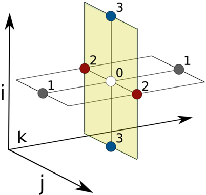
The 7-point stencil (Figure 2) defines the result at r i,j,k as a linear combination of the input a i,j,k and its six three-dimensional neighbors with Manhattan distance one. The 27point stencil uses a linear combination of the set of 26 neighbors with Chebyshev distance one. The boundary values r i,j,k with i ∈ { 0 , M -1 } , j ∈ { 0 , N -1 } , or k ∈ { 0 , P -1 } are not written as is standard for Dirichlet boundary conditions. Other boundary conditions would apply a different one-sided stencil at these location, a computationally inexpensive consideration that we do not regard for our experiments.
Figure 2: 7-point stencil operator
<details>
<summary>Image 1 Details</summary>
### Visual Description
\n
## Diagram: 3D Coordinate System with Points
### Overview
The image depicts a 3D coordinate system with three axes labeled 'i', 'j', and 'k'. A plane is shown intersecting the coordinate system, and several points are marked within and around this space. The points are numbered 0 through 3, and colored white, red, and dark blue/gray.
### Components/Axes
* **Axes:** The diagram features three orthogonal axes:
* 'i' - Points upwards along the vertical axis.
* 'j' - Points diagonally downwards and to the right.
* 'k' - Points diagonally to the right.
* **Plane:** A pale yellow plane cuts through the 3D space, not aligned with any of the primary axes.
* **Points:** Six points are visible, labeled with numbers 0-3 and colored as follows:
* Point 0: White
* Points 2: Red (two instances)
* Points 1: Gray (two instances)
* Points 3: Dark Blue/Gray (two instances)
### Detailed Analysis / Content Details
The points are positioned as follows:
* **Point 0:** Located at the approximate center of the coordinate system and within the plane.
* **Point 1 (Gray):** Located to the left of the coordinate system, outside the plane. Appears to be at approximately (-1, 0, 0) relative to the origin.
* **Point 1 (Gray):** Located to the right of the coordinate system, outside the plane. Appears to be at approximately (1, 0, 0) relative to the origin.
* **Point 2 (Red):** Located within the plane, slightly below the center. Appears to be at approximately (0, -1, 0) relative to the origin.
* **Point 2 (Red):** Located within the plane, slightly above the center. Appears to be at approximately (0, 1, 0) relative to the origin.
* **Point 3 (Dark Blue/Gray):** Located below the plane. Appears to be at approximately (0, 0, -1) relative to the origin.
* **Point 3 (Dark Blue/Gray):** Located above the plane. Appears to be at approximately (0, 0, 1) relative to the origin.
### Key Observations
* Point 0 is centrally located.
* Points 1, 2, and 3 appear to be arranged symmetrically around the origin, but are not necessarily equidistant.
* The plane does not align with any of the coordinate axes.
* The points are positioned in a way that suggests they might represent vertices or key locations within the defined 3D space.
### Interpretation
The diagram likely illustrates a geometric concept or a coordinate transformation. The plane could represent a subspace or a projection of a higher-dimensional space. The points could represent vectors, data points, or nodes within a system. The arrangement of the points suggests a possible relationship to the coordinate axes and the plane, potentially demonstrating a mapping or transformation between different coordinate systems. The use of different colors for the points might indicate different properties or classifications. Without further context, it's difficult to determine the precise meaning of the diagram, but it clearly represents a spatial arrangement within a 3D coordinate system. The diagram is a visual aid for understanding spatial relationships and potentially linear algebra concepts.
</details>
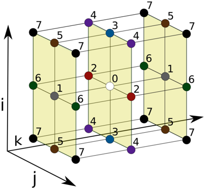
The 27-point stencil (Figure 3) can be seen as the summation over nine independent 3-point stencil operators into a single result. We assume symmetry along but not between the three dimensions, leading to 8 unique weight coefficients. The symmetric 7-point stencil operator has 4 unique weight coefficients.
## 3.2 PowerPC 450
Designed for delivering power-efficient floating point computations, the nodes in a Blue Gene/P system are four-way Symmetric Processors (SMPs) comprised of PowerPC 450 processing cores [21]. The processing cores possess a modest superscalar architecture capable of issuing a SIMD floating point instruction in parallel with various integer and load/store instructions. Each core has an independent register file containing 32 4-byte general purpose registers and 32 16-byte SIMD floating point registers which are operated on by a pair of fused floating point units. A multiplexing unit on each end of this chained floating point pipeline enables a rich combination of parallel, copy, and cross semantics in the SIMD floating point operation set. This flexibility in the multiplexing unit can enhance computational efficiency by replacing the need for independent copy and swap operations on the floating point registers with single operations. To provide backward compatibility as well as some additional functionality, these 16-byte SIMD floating point registers are divided into independently addressable, 8-byte primary and secondary registers wherein non-SIMD floating point instructions operate transparently on the primary half of each SIMD register.
An individual PowerPC 450 core has its own 64KB L1 cache, divided evenly into a 32KB instruction cache and a 32KB data cache. The L1 data cache uses a round-robin (First In First Out (FIFO)) replacement policy in 16 sets, each with 64-way set-associativity. Each L1 cache line is 32 bytes in size.
Every core also has its own private prefetch unit, designated as the L2 cache, 'between' the L1 and the L3. In the default configuration, each PowerPC 450 core can support up to 5 'deep fetching' streams or up to 7 shallower streams. These values stem from the fact that the L2 prefetch cache has 15 128-byte entries. If the system is fetching two lines ahead (settings are configured on job startup), each stream occupies three positions, one current and two 'future,' while a shallower prefetch lowers the occupancy to two per stream. The final level of cache is the 8MB L3, shared among the four cores. The L3 features a Least Recently Used (LRU) replacement policy, with 8-way set associativity and a 128-byte line size.
Figure 3: 27-point stencil operator
<details>
<summary>Image 2 Details</summary>
### Visual Description
\n
## Diagram: 3D Coordinate System with Numerical Labels
### Overview
The image depicts a three-dimensional coordinate system, resembling a cube constructed from lines. Each vertex of the cube is labeled with a numerical value ranging from 0 to 7. The axes are labeled 'i', 'j', and 'k', indicating a standard Cartesian coordinate system. The diagram appears to illustrate a mapping of numerical values to specific points within a 3D space.
### Components/Axes
* **Axes:** Three axes are present, labeled 'i' (vertical, pointing upwards), 'j' (horizontal, pointing towards the viewer), and 'k' (horizontal, pointing to the right).
* **Vertices:** The cube has 8 vertices, each marked with a black circle and a numerical label.
* **Numerical Labels:** The labels range from 0 to 7.
* **Color Coding:** Some vertices are colored differently:
* Red
* Blue
* Purple
* Green
* Gray
* Brown
### Detailed Analysis / Content Details
The diagram shows a cube with each corner labeled with a number. The numbers appear to be assigned in a consistent, though not immediately obvious, pattern.
Here's a breakdown of the vertex labels and their approximate positions:
* **(0,0,0):** Label '0', located at the center of the cube. (White circle)
* **(0,0,7):** Label '7', located at the top-right-back corner. (Black circle)
* **(0,7,0):** Label '6', located at the top-left-back corner. (Green circle)
* **(0,7,7):** Label '6', located at the top-right-front corner. (Green circle)
* **(7,0,0):** Label '5', located at the bottom-right-back corner. (Brown circle)
* **(7,0,7):** Label '5', located at the bottom-right-front corner. (Brown circle)
* **(7,7,0):** Label '1', located at the bottom-left-back corner. (Gray circle)
* **(7,7,7):** Label '7', located at the bottom-right-front corner. (Black circle)
Additionally, there are intermediate points within the cube, also labeled:
* **(0,2,0):** Label '2', (Red circle)
* **(0,2,7):** Label '2', (Red circle)
* **(0,4,3):** Label '3', (Blue circle)
* **(0,4,4):** Label '4', (Purple circle)
* **(7,1,6):** Label '1', (Gray circle)
* **(7,3,4):** Label '4', (Purple circle)
* **(7,5,0):** Label '7', (Black circle)
* **(7,5,7):** Label '7', (Black circle)
* **(7,6,2):** Label '2', (Red circle)
* **(7,6,6):** Label '6', (Green circle)
### Key Observations
* The numbers are not simply coordinates.
* The color coding doesn't appear to be directly related to the numerical value.
* The labeling seems to follow a pattern, but it's not a simple linear progression along any single axis.
* The central point (0,0,0) is uniquely labeled '0' and is the only white circle.
### Interpretation
This diagram likely represents a discrete mapping of values within a 3D space. The numbers could represent any kind of data associated with each point in the cube – for example, density, temperature, or a state in a system. The color coding might represent categories or classifications of these values.
The pattern of labeling suggests a possible underlying function or algorithm that assigns these values to the points. Without further context, it's difficult to determine the exact nature of this function. The diagram could be a visualization of a data structure, a simulation result, or a conceptual model.
The fact that some numbers are repeated (e.g., '7' appears multiple times) suggests that the mapping is not necessarily one-to-one. The diagram is a visual representation of a mathematical or computational concept, but its specific meaning requires additional information. It is a visual representation of a discrete space, and the numbers represent some property of each location within that space.
</details>
On this architecture the desired scenario in highly performant numerical codes is the dispatch of a SIMD floating point instruction every cycle (in particular, a SIMD Floating point Multiply-Add (FMA)), with any load or store involving one of the floating point registers issued in parallel, as inputs are streamed in and results are streamed out. Floating point instructions can be retired one per cycle, yielding a peak computational throughput of one (SIMD) FMA per cycle, leading to a theoretical peak of 3.4 GFlops/s per core. Blue Gene/P's floating point load instructions, whether they be SIMD or non-SIMD, can be retired every other cycle, leading to an effective read bandwidth to the L1 of 8 bytes a cycle for aligned 16-byte SIMD loads (non-aligned loads result in a significant performance penalty) and 4 bytes a cycle otherwise. As a consequence of the instruction costs, no kernel can achieve peak floating point performance if it requires a ratio of load to SIMD floating point instructions greater than 0.5. It is important to ensure packed 'quad-word' SIMD loads occur on 16-byte aligned memory boundaries on the PowerPC 450 to avoid performance penalties that ensue from the hardware interrupt that results from misaligned loads or stores.
An important consideration for achieving high throughput performance on modern floating point units is pipeline latency, the number of cycles that must transpire between accesses to an operand being written or loaded into in order to avoid pipeline hazards (and their consequent stalls). Floating point computations on the PowerPC 450 have a latency of 5 cycles, whereas double-precision loads from the L1 require at least 4 cycles and those from the L2 require approximately 15 cycles [38]. Latency measurements when fulfilling a load request from the L3 or DDR memory banks are less precise: in our performance modeling we assume an additional 50 cycle average latency penalty for all loads outside the L1 that hit in the L3.
In the event of an L1 cache miss, up to three concurrent requests for memory beyond the L1 can execute (an L1 cache miss while 3 requests are 'in-flight' will cause a stall until one of the requests to the L1 has been fulfilled). Without assistance from the L2 cache, this leads to a return of 96 bytes (three 32-byte lines) every 56 cycles (50 cycles of memory latency + 6 cycles of instruction latency), for an effective bandwidth of approximately 1.7 bytes/cycle. This architectural characteristic is important in our work, as L3-confined kernels with a limited number of streams can effectively utilize the L2 prefetch cache and realize as much as 4.5 bytes/cycle bandwidth per core, while those not so constrained will pay the indicated bandwidth penalty.
The PowerPC 450 is an in-order unit with regards to floating point instruction execution. An important consequence is that a poorly implemented instruction stream featuring many non-interleaved load/store or floating point operations will suffer from frequent structural hazard stalls with utilization of only one of the units. Conversely, this in-order nature makes the result of efforts to schedule and bundle instructions easier to understand and extend.
## 3.3 Instruction Scheduling Optimization
We wish to minimize the required number of cycles to execute a given code block composed of PowerPC 450 assembly instructions. This requires scheduling (reordering) the instructions of the code block to avoid the structural and data hazards described in the previous section. Although we use greedy heuristics in the current implementation of the code synthesis framework to schedule instructions, we can formulate the scheduling problem as an Integer Linear Programming (ILP) optimization problem. We base our formulation on [7], which considers optimizations combining register allocation and instruction scheduling of architectures with multi-issue pipelines. To account for multi-cycle instructions, we include parts of the formulation in [41]. We consider two minor extensions to these approaches. First, we consider the two separate sets of registers of the PowerPC 450, the General Purpose Registers (GPR), and the Floating Point Registers (FPR). Second, we account for instructions that use the Load Store Unit (LSU) occupying the pipeline for a varying number of cycles.
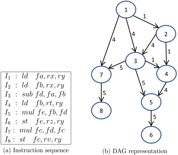
We begin by considering a code block composed of N instructions initially ordered as I = { I 1 , I 2 , I 3 , ..., I N } . A common approach to represent the data dependencies of these instructions is to use a Directed Acyclic Graph (DAG). Given a DAG G ( V, E ), the nodes of the graph ( V ) represent the instructions and the directed edges ( E ) represent the dependencies between them. Figure 4 shows an example of a DAG representing a sequence of instructions with the edges representing data dependencies between instructions. Each read-after-write data dependency of an instruction I j on an instruction I i is represented by a weighted edge e ij . This weighted edge corresponds to the number of cycles needed by an instruction I i to produce the results required by an instruction I j . The weights associated with write-after-read and write-after-write data dependencies are set to one.
Figure 4: Example of DAG representation of the instructions
<details>
<summary>Image 3 Details</summary>
### Visual Description
\n
## Diagram: Instruction Sequence and Directed Acyclic Graph (DAG) Representation
### Overview
The image presents a comparison between an instruction sequence (a list of assembly-like instructions) and its corresponding Directed Acyclic Graph (DAG) representation. The instruction sequence is labeled "(a)", and the DAG is labeled "(b)". The DAG visually depicts the dependencies between the instructions.
### Components/Axes
The image consists of two main components:
1. **Instruction Sequence:** A vertically aligned list of eight instructions, labeled I1 through I8. Each instruction is formatted as "Instruction : operands".
2. **DAG Representation:** A graph composed of nodes (numbered 1 through 8) and directed edges representing dependencies.
### Content Details
**Instruction Sequence (a):**
* I1 : ld fa, rx, ry
* I2 : ld fb, rx, ry
* I3 : sub fd, fa, fb
* I4 : ld fb, rt, ry
* I5 : mul fe, fb, fd
* I6 : st fe, rz, ry
* I7 : mul fc, fd, fc
* I8 : st fc, rv, ry
**DAG Representation (b):**
The DAG consists of 8 nodes, numbered 1 to 8. The edges indicate dependencies.
* Node 1 has outgoing edges to nodes 2 and 3, with edge weights of 1 and 4 respectively.
* Node 2 has an outgoing edge to node 4 with a weight of 4.
* Node 3 has outgoing edges to nodes 4, 5, and 7 with weights of 1, 5, and 5 respectively.
* Node 4 has an outgoing edge to node 5 with a weight of 4.
* Node 5 has an outgoing edge to node 6 with a weight of 5.
* Node 7 has an outgoing edge to node 8 with a weight of 5.
* Node 8 has no outgoing edges.
The nodes represent the instructions, and the edges represent data dependencies. For example, the edge from node 1 to node 3 indicates that instruction I3 depends on the result of instruction I1.
### Key Observations
* The DAG visually demonstrates the order in which instructions can be executed, taking dependencies into account.
* Instructions I1 and I2 (ld fa, rx, ry and ld fb, rx, ry) can be executed in parallel as they are both sources.
* Instruction I8 (st fc, rv, ry) is the final instruction, as it has no outgoing edges.
* The edge weights represent the latency or cost associated with the dependency.
### Interpretation
The image illustrates the concept of instruction-level parallelism and how a DAG can be used to represent and optimize instruction scheduling. The DAG allows for identifying independent instructions that can be executed concurrently, potentially improving performance. The weights on the edges suggest that some dependencies are more costly (take longer) than others. The DAG representation is a common technique used in compilers and processors to optimize code execution. The diagram shows how a linear sequence of instructions can be transformed into a graph that reveals opportunities for parallel execution. The DAG is a visual tool for understanding data flow and dependencies within a program.
</details>
The PowerPC 450 processor has one LSU and one FPU. This allows the processor to execute a maximum of one floating point operation per cycle and one load/store operation every two cycles (each operation using the LSU consumes at least 2 cycles). The instructions use either the LSU ( I LSU ∈ LSU ) or the other computation resources of the processor including the FPU ( I FPU ∈ FPU ). A critical path, C , in the DAG is a path in the graph on which the sum of the edge weights attains the maximum. We can compute the lower bound
( L bound ) to run the instructions I as follows:
$$F P U _ { 1 } ^ { \prime } ( 1 )$$
We can compute an upper bound U bound ( I ) by simulating the number of cycles to execute the scheduled instructions. If U bound ( I ) = L bound ( I ) we can generate an optimal schedule.
We define the Boolean optimization variables x j i to take the value 1 to represent that the instruction I i is scheduled at a given cycle c j and 0 otherwise. These variables are represented in the array shown in Figure 5, where M represents the total number of the cycles.
Figure 5: A Boolean array of size N × M representing the scheduling variables
| | c 1 | c 2 | c 3 | . | c M |
|-----|-------|-------|-------|-----|-------|
| I 1 | x 1 1 | x 2 1 | x 3 1 | . | x M 1 |
| I 2 | x 1 2 | x 2 2 | x 3 2 | . | x M 2 |
| I 3 | x 1 3 | x 2 3 | x 3 3 | . | x M 3 |
| . | . | . | . | . | . |
| I N | x 1 N | x 2 N | x 3 N | . | x M N |
The first constraint in our optimization is to force each instruction to be scheduled only once in the code block. Formally:
$$\sum _ { j = 1 } ^ { M } x _ { i } = 1 , \forall i \in \{ 1 , 2 , \ldots , N \}$$
The PowerPC 450 processor can execute a maximum of one floating point operation every cycle and one load operation every two cycles (store instructions are more complicated, but for this derivation we assume two cycles as well). This imposes the following constraints:
$$\sum _ { i : I \in [ 1 , M ] } x ^ { i } \leq 1 , V _ { j }$$
$$\sum _ { i : 1 \leq i \leq LSU } ( x ^ { i } + x ^ { j + 1 } )$$
Finally, to maintain the correctness of the code's results we enforce the dependency constraints:
$$\sum _ { k = 1 } ^ { M } \sum _ { i = 1 } ^ { k } ( k * x ^ { j } ) - \sum _ { k = 1 } ^ { M } ( k$$
The instruction latency to write to a GPR is 1 cycle ( e ij = 1). The latency for writing to a FPR is 5 cycles for I i ∈ I FPU and at least 4 cycles for I i ∈ I LSU . Load instructions have higher latency when the loaded data is present in the L3 cache or the RAM. This can be considered in future formulations to maximize the number of cycles between loading the data of an instruction I i and using it by maximizing e ij in the objective.
We also wish to constrain the maximum number of allocated registers in a given code block. All the registers are assumed to be allocated and released within the code block. An instruction I i scheduled at a cycle c j allocates a register r by writing on it. The register r is released (deallocated) at a cycle c k by the last instruction reading from it. The life span of the register r is defined to be from cycle c j to cycle c k inclusive.
We define two sets of Boolean register optimization variables g j i and f j i to represent the usage of the GPR and the FPR files, respectively. Each of these variables belongs to an array of the same size as the array in Figure 5. The value of g j i is set to 1 during the life span of a register in the GPR modified by the instruction I i scheduled at the cycle c j and last read by an instruction scheduled at the cycle c k , that is g z i = 1 when j ≤ z ≤ k and zero otherwise. The same applies to the variables f j i to represent the FPR register allocation.
To compute the values of g j i and f j i , we define the temporary variables ˆ g p i and ˆ f p i . Let K i be the number of instructions reading the from the register allocated by the instruction I i . These temporary variables are computed as follows:
$$f _ { i } = K \sum _ { z = 1 } ^ { p } x _ { i } - v$$
$$g _ { i } = K \sum _ { z = 1 } ^ { p } x _ { i } ^ { z } - v$$
Our optimization variables g j i and f j i will equal to 1 only when ˆ g j i > 0 and ˆ f j i > 0, respectively. This can be formulated as follow:
$$f _ { i } - f _ { j } \leq 0$$
$$g _ { i } - g _ { j } \leq 0$$
$$( 1 )$$
$$\vert k \vert = \vert g _ { i } \vert - \vert g _ { j } \vert \geq 0$$
Now we can constrain the maximum number of used registers FPR max and GPR max by the following:
$$\sum _ { i = 1 } ^ { N } ( g _ { j } ) - G P R _ { m a }$$
$$\sum _ { i = 1 } ^ { N } ( f _ { j } ) - F P R _ { m a }$$
Our optimization objective is to minimize the required cycles to execute the code ( C run ). The complete formulation of the optimization problem is:
$$\frac { 1 } { n } \sum _ { k = 1 } ^ { n } a _ { k }$$
$$Subject to:$$
$$\sum _ { j = 1 } ^ { M } x _ { i , j } = 1 , \forall i \in \{ 1 , 2 , \ldots , N \}$$
$$\sum _ { i : I \in F P U } x _ { i } \leq 1 , v _ { j }$$
$$\sum _ { i : I \in [ 1 , 2 , \ldots , M - 1 ] } ( x ^ { i } + x ^ { j } + 1 )$$
$$\sum _ { i = 1 } ^ { M } \sum _ { j = 1 } ^ { k } ( k * x _ { i } ) - \sum _ { i = 1 } ^ { M } ( k = 1$$
$$\sum _ { i = 1 } ^ { N } ( g _ { j } ) - G P R _ { m a 3 }$$
$$\sum _ { i = 1 } ^ { N } ( f _ { j } ) - F P R _ { m a x }$$
$$\sum _ { j = 1 } ^ { M } j * x _ { i } - C _ { run } \sum$$
The general form of this optimization problem is known to be NP-complete [19], although many efficient implementations exist for solving integer problems exist; no known algorithms can guarantee global solutions in polynomial time. In our implementation, we use a greedy algorithm that yields an approximate solution in practical time as we describe in 4.4.
## 4 Implementation
## 4.1 C and Fortran
We implement the three streaming kernels in C and Fortran and utilize published results as a benchmark to gain a better understanding of the relative performance of the general class of streaming numerical kernels on the IBM PowerPC 450. Our first challenge is in expressing a SIMDized mapping of the stencil operator in C or Fortran. Neither language natively supports the concept of a unit of SIMD-packed doubles, though Fortran's complex type comes very close. Complicating matters further, the odd cardinality of the stencil operators necessitates careful tactics to efficiently SIMDize the code. Regardless of the unrolling strategy employed, one of every two loads is unaligned or requires clever register manipulation. It is our experience that standard C and Fortran implementations of our stencil operators will compile into exclusively scalar instructions that cannot attain greater than half of peak floating point performance. For example, with a na¨ ıve count of 53 flops per 27-point stencil, peak performance is 62 Mstencil/s and we observe 31.5 Mstencil/s on a single core of the PowerPC 450. Register pressure and pipeline stalls further reduce the true performance to 21.5 Mstencil/s. We note that Datta [11] was able to improve this to 25 Mstencil/s using manual unrolling, common subexpression elimination, and other optimizations within C.
The XL compilers support intrinsics which permit the programmer to specify which instructions are used, but the correspondence between intrinsics and instructions is not exact enough for our purposes. The use of intrinsics can aid programmer productivity, as this method relies upon the compiler for such tasks as register allocation and instruction scheduling. However, our methods require precise control of these aspects of the produced assembly code, making this path unsuitable for our needs.
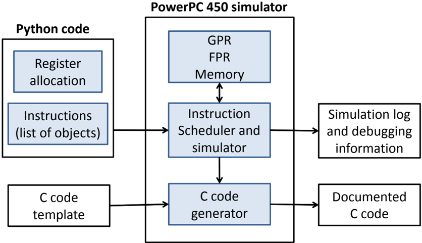
Our code generation framework is shown in Figure 6. High-level Python code produces the instruction sequence of each code block. First, registers are allocated by assigning them variable names. Next, a list of instruction objects is created that utilize the variables to address registers. Enabling the instruction scheduler allows the simulator to execute the instructions out of order; otherwise they will be executed in order. The instruction simulator uses virtual GPR, FPR, and memory to simulate the pipeline execution and to simulate the expected results of the given instruction sequence. A log is produced by the instruction simulator to provide the simulation details, showing the cycles at which the instructions are scheduled and any encountered data and structural hazards. Also, the log can contain the contents of the GPR, the FPR, and the memory, at any cycle, to debug the code for results correctness. The C code generator takes the simulated instructions and generates their equivalent inline assembly code in a provided C code template using the inline assembly extension to C standard provided by GCC. For added clarity, we associate each generated line with a comment showing the mapping between the used registers numbers and their corresponding variables names in the Python code.
Figure 6: The components of the code generation framework in this work
<details>
<summary>Image 4 Details</summary>
### Visual Description
\n
## Diagram: PowerPC 450 Simulator Architecture
### Overview
The image depicts a block diagram illustrating the architecture of a PowerPC 450 simulator. The diagram shows the flow of data and control between different components, starting with Python code and culminating in documented C code and simulation logs. The diagram is divided into two main sections: the input side (Python code) and the simulator itself (PowerPC 450 simulator).
### Components/Axes
The diagram consists of the following components:
* **Python code:** This section contains two components:
* Register allocation
* Instructions (list of objects)
* **PowerPC 450 simulator:** This is the central block, containing:
* GPR (General Purpose Registers)
* FPR (Floating Point Registers)
* Memory
* Instruction Scheduler and simulator
* C code generator
* **Output:** This section contains two components:
* Simulation log and debugging information
* Documented C code
* **C code template:** This is an input to the C code generator.
Arrows indicate the direction of data flow between these components.
### Detailed Analysis / Content Details
The diagram shows the following data flow:
1. **Python code** (Register allocation and Instructions) feeds into the **Instruction Scheduler and simulator** within the PowerPC 450 simulator.
2. The **Instruction Scheduler and simulator** interacts with **GPR**, **FPR**, and **Memory** (represented as a nested block within the simulator). There is bidirectional flow between the Instruction Scheduler and Memory.
3. The **Instruction Scheduler and simulator** outputs to the **C code generator**.
4. The **C code generator** also receives input from a **C code template**.
5. The **C code generator** outputs **Documented C code**.
6. The **Instruction Scheduler and simulator** also outputs **Simulation log and debugging information**.
The components within the PowerPC 450 simulator (GPR, FPR, Memory) are visually grouped together, suggesting they form a core functional unit. The arrows indicate a sequential processing flow, where Python code is translated into instructions, simulated, and then converted into C code.
### Key Observations
The diagram highlights the key stages of the simulation process: instruction scheduling, simulation, and code generation. The inclusion of a C code template suggests that the generated C code is based on a predefined structure. The output of simulation logs and debugging information indicates that the simulator provides tools for analyzing and understanding the simulation process.
### Interpretation
This diagram illustrates a software architecture for simulating a PowerPC 450 processor. The use of Python as an input language suggests a high-level scripting approach for defining the simulation parameters and instructions. The simulator itself appears to be implemented in a combination of hardware-like components (GPR, FPR, Memory) and software modules (Instruction Scheduler, C code generator). The generation of C code as an output suggests that the simulator can be used to translate PowerPC 450 instructions into a more portable and executable format. The simulation logs and debugging information are crucial for verifying the correctness and performance of the simulation.
The diagram suggests a layered approach to simulation, where high-level Python code is translated into low-level instructions, simulated on a virtual processor, and then converted into C code for further analysis or execution. This architecture allows for flexibility in defining the simulation environment and provides tools for debugging and understanding the simulation process. The diagram does not provide any quantitative data or performance metrics, but it clearly outlines the functional components and data flow of the PowerPC 450 simulator.
</details>
## 4.2 Kernel Design
The challenges in writing fast kernels in C and Fortran motivate us to program at the assembly level, a (perhaps surprisingly) productive task when using our code synthesis framework: an experienced user was able to design, implement, and test several efficient kernels for a new stencil operator in one day using the framework. Much of our work is based on the design of two small and na¨ ıvely scheduled, 3-point kernels, dubbed mutate-mutate and load-copy, that we introduce in 4.2. The kernels distinguish themselves from each other by their relative balance between load/store and floating point cycles consumed per stencil.
We find that efficiently utilizing SIMD units in stencil computations is a challenging task. To fill the SIMD registers, we pack two consecutive data elements from the fastest moving dimension, k , allowing us to compute two stencils simultaneously, as in [2]. Computing in this manner is semantically equivalent to an unrolling by 2 in the k direction. As a connventional notation, since i and j are static for any given stream, we denote the two values occupying the SIMD register for a given array by their k indices, e.g., SIMD register a 34 contains A i,j, 3 in its primary half and A i,j, 4 in its secondary half.
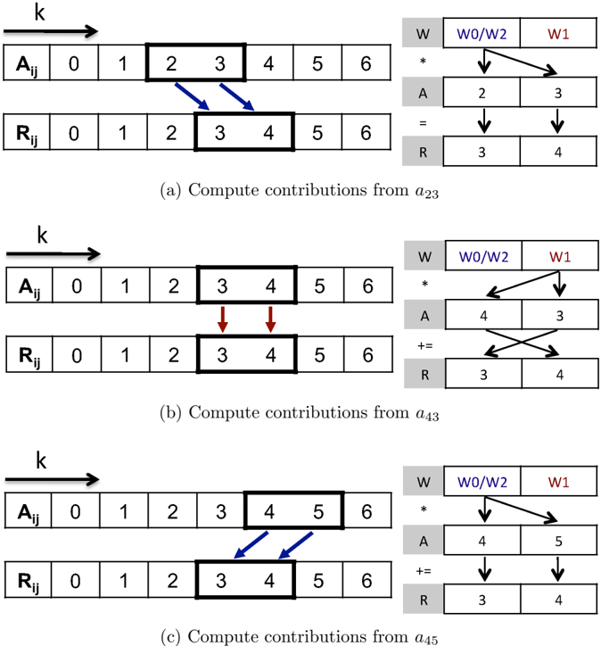
Many stencil operators map a subset of adjacent A elements with odd cardinality to each R element, as is illustrated in the left half of Figure 7, which depicts the SIMD register contents and computations mid-stream of a 3-point kernel. The odd cardinality prevents a straightforward mapping from SIMD input registers to SIMD output registers. We note that aligned SIMD loads from A easily allow for the initialization of registers containing a 23 and a 45 . Similarly, the results in r 34 can be safely stored using a SIMD store. The register containing a 34 , unaligned elements common to the aligned registers containing adjacent data, requires a shuffle within the SIMD registers through the use of additional load or floating point move instructions.
We introduce two kernels, which we designate as mutate-mutate (mm) and load-copy (lc), as two different approaches to form the packed data into the unaligned SIMD registers while streaming through A in memory. A 'mutate' operation is defined as the replacment of one operand of a SIMD register by a value loaded from memory. A 'load' operation is defined as the replacement of both operands in a SIMD register by a SIMD load from memory. A 'copy' operation is the replacement of one operand of a SIMD register by an operand from another SIMD register. Mutates and loads utilize the LSU, copies utilize the FPU.
The mutate-mutate kernel replaces the older half of the SIMD register by with the next element of the stream. In our example in Figure 7 we start with a 23 loaded in the SIMD register, then after the first computation we load a 4 into the primary part of the SIMD register so that the full contents are a 43 .
The load-copy kernel instead combines the unaligned values in a SIMD register from two consecutive aligned quad-words loaded in two SIMD registers by copying, the primary element from the second register to the primary element of the first. In our example a 23 and a 45 are loaded in two SIMD registers. Then, after the needed computations involving a 23 have been dispatched, a floating point move instruction replaces a 2 with a 4 to form a 43 .
The two kernels use an identical set of floating point instructions, visually depicted in the right half of Figure 7, to accumulate the computations into the result registers. The two needed weight coefficients are packed into one SIMD register. The first floating point
Figure 7: SIMD stencil computations on one-dimensional streams
<details>
<summary>Image 5 Details</summary>
### Visual Description
\n
## Diagram: Matrix Decomposition Illustration
### Overview
The image presents a series of three diagrams illustrating a matrix decomposition process, likely related to collaborative filtering or a similar technique. Each diagram shows two matrices, denoted as A<sub>ij</sub> and R<sub>ij</sub>, along with a calculation involving a vector W. The diagrams demonstrate how elements of matrix R are updated based on elements of matrix A and vector W.
### Components/Axes
Each diagram consists of:
* **Matrix A<sub>ij</sub>**: A 7x7 matrix with row and column indices ranging from 0 to 6. The horizontal axis is labeled "k".
* **Matrix R<sub>ij</sub>**: A 7x7 matrix with row and column indices ranging from 0 to 6.
* **Vector W**: A vector with elements W0, W1, and W2.
* **Arrows**: Blue arrows indicate the elements of A<sub>ij</sub> used in the calculation. Red arrows indicate the elements of R<sub>ij</sub> being updated.
* **Calculation Block**: A block showing the multiplication and addition operations performed using elements from A<sub>ij</sub>, R<sub>ij</sub>, and W.
* **Sub-captions**: Each diagram has a caption indicating which elements of A are being used for the computation: (a) a<sub>23</sub>, (b) a<sub>43</sub>, (c) a<sub>45</sub>.
### Detailed Analysis or Content Details
**Diagram (a): Compute contributions from a<sub>23</sub>**
* **Matrix A<sub>ij</sub>**: Values are not explicitly shown, but the cells are shaded.
* **Matrix R<sub>ij</sub>**: Values are not explicitly shown, but the cells are shaded.
* **Calculation Block**:
* A = 2 (bottom left)
* R = 3 (bottom right)
* W = [W0/W2, W1] (top)
* The calculation shows A multiplied by W0/W2, resulting in 2, and added to R, resulting in 3.
**Diagram (b): Compute contributions from a<sub>43</sub>**
* **Matrix A<sub>ij</sub>**: Values are not explicitly shown, but the cells are shaded.
* **Matrix R<sub>ij</sub>**: Values are not explicitly shown, but the cells are shaded.
* **Calculation Block**:
* A = 4 (bottom left)
* R = 3 (bottom right)
* W = [W0/W2, W1] (top)
* The calculation shows A multiplied by W0/W2, resulting in 4, and added to R, resulting in 3.
**Diagram (c): Compute contributions from a<sub>45</sub>**
* **Matrix A<sub>ij</sub>**: Values are not explicitly shown, but the cells are shaded.
* **Matrix R<sub>ij</sub>**: Values are not explicitly shown, but the cells are shaded.
* **Calculation Block**:
* A = 4 (bottom left)
* R = 3 (bottom right)
* W = [W0/W2, W1] (top)
* The calculation shows A multiplied by W0/W2, resulting in 4, and added to R, resulting in 3.
### Key Observations
* The diagrams illustrate an iterative process where elements of R are updated based on corresponding elements of A and a weight vector W.
* The calculation involves multiplying an element of A by W0/W2 and adding it to the corresponding element of R.
* The specific elements of A used in each diagram (a<sub>23</sub>, a<sub>43</sub>, a<sub>45</sub>) suggest a specific order or pattern in the decomposition process.
* The values in the calculation blocks (A=2, R=3, A=4, R=3, A=4, R=3) are consistent across the diagrams, but the specific elements of A being used change.
### Interpretation
The diagrams demonstrate a step in a matrix factorization or decomposition algorithm. The matrix A likely represents user-item interactions or preferences, while R is an intermediate matrix being constructed. The vector W represents weights or factors used in the decomposition. The process shown involves updating elements of R by incorporating information from A, weighted by W. This is a common technique in collaborative filtering, where the goal is to predict missing values in A (e.g., user preferences for items they haven't rated) by decomposing A into lower-dimensional matrices. The specific choice of elements (a<sub>23</sub>, a<sub>43</sub>, a<sub>45</sub>) and the consistent values in the calculation blocks suggest a specific implementation or optimization strategy within the algorithm. The use of W0/W2 suggests a potential normalization or scaling factor. The diagrams are illustrative and do not provide specific numerical values for the matrix elements, but they clearly demonstrate the underlying process of updating R based on A and W.
</details>
operation is a cross copy-primary multiply instruction, multiplying two copies of the first weight coefficient by the two values in a 23 , then placing the results in the SIMD register containing r 34 (Figure 7a). Then, the value of a 23 in the SIMD register is modified to become a 43 , replacing one data element in the SIMD register either through mutate or copy. The second floating point operation is a cross complex multiply-add instruction, performing a cross operation to deal with the reversed values (Figure 7b). Finally, the value a 45 , which has either been preloaded by load-copy or is created by a second mutation in mutate-mutate, is used to perform the last computation (Figure 7c).
We list the resource requirements of the load-copy and the mutate-mutate kernels in Table 1. The two kernels are at complementary ends of a spectrum. The mutate-mutate kernel increases pressure exclusively on the load pipeline while the load-copy kernel incurs extra cycles on the floating point unit. The two strategies can be used in concert, using mutate-mutate when the floating point unit is the bottleneck and the load-copy when it is not.
Table 1: Resource usage per stencil of mutate-mutate and load-copy
| Kernel | Operations | Operations | Cycles | Cycles | Registers | Registers |
|---------------|--------------|--------------|----------|----------|-------------|-------------|
| | ld-st | FPU | ld-st | FPU | Input | Output |
| mutate-mutate | 2-1 | 3 | 6 | 3 | 1 | 1 |
| load-copy | 1-1 | 4 | 4 | 4 | 2 | 1 |
## 4.3 Unroll-and-Jam
The 3-point kernels are relatively easy to specify in assembly, but the floating point and load/store instruction latencies will cause pipeline stalls if they are not unrolled. Further unrolling in the k -direction beyond two is a possible solution that we do not explore in this paper. Although this solution would reduce the number of concurrent memory streams, it would also reduce data reuse for the other stencils studied in this paper.
Unrolling and jamming once in transverse directions provides independent arithmetic operations to hide instruction latency, but interleaving the instructions by hand produces large kernels that are difficult to understand and modify. To simplify the design process, we constructed a synthetic code generator and simulator with reordering capability to interleave the jammed FPU and load/store instructions to minimize pipeline stalls. The synthetic code generator also gives us the flexibility to implement many general stencil operators, including the 7-point and 27-point stencils using the 3-point stencil as a building block.
Unroll-and-jam serves a second purpose for the 7-point and 27-point stencil operators due to the overlapped data usage among adjacent stencils. Unroll-and-jam eliminates redundant loads of common data elements among the jammed stencils, reducing pressure on the memory subsystem by increasing the effective arithmetic intensity of the kernel. This can be quantified by comparing the number of input streams, which we refer to as the 'frame size,' with the number of output streams. For example, an unjammed 27-point stencil requires a frame size of 9 input streams for a single output stream. If we unroll once in i and j , we generate a 2 × 2 jam with 4 output streams using a frame size of 16, improving the effective arithmetic intensity by a factor of 9 4 .
We used mutate-mutate and load-copy kernels to construct 3-, 7-, and 27-point stencil kernels over several different unrolling configurations. Table 2 lists the register allocation requirements for these configurations and provides per-cycle computational requirements. In both the mutate-mutate and load-copy kernels, the 27-point stencil is theoretically FPUbound because of the high reuse of loaded input data elements across streams.
As can be seen in Table 1, the mutate-mutate kernel allows more unrolling for the 27-point stencil than the load-copy kernel because it uses fewer registers per stencil. The number of allocated registers for input data streams at the mutate-mutate kernel is equal to the number of the input data streams, while the load-copy kernel requires twice the number of registers for its input data streams.
## 4.4 PowerPC 450 Simulator
The high-level code synthesis technique generates as many as hundreds of assembly instructions with aggressive unrolling. For optimal performance, we greedily schedule the assembly
Table 2: Computational requirements
| 3-lc-2x4 | 3-lc-2x3 | 3-lc-2x2 | 3-lc-2x1 | 3-lc-1x1 | 7-lc-2x3 | 7-mm-2x3 | 27-mm-2x3 | 27-mm-2x2 | 27-mm-1x3 | 27-mm-1x2 | 27-mm-1x1 | | Kernel |
|------------|------------|------------|------------|------------|------------|------------|-------------|-------------|-------------|-------------|-------------|---------------------|---------------------|
| 8 | 6 | 4 | 2 | 1 | 16 | 16 | 20 | 16 | 15 | 12 | 9 | Frame | Configurations |
| 16 | 12 | 8 | 4 | 2 | 12 | 12 | 12 | 8 | 6 | 4 | 2 | Stencils/ Iteration | |
| 16 | 12 | 8 | 4 | 2 | 22 | 16 | 20 | 16 | 15 | 12 | 9 | | Input |
| 8 | 6 | 4 | 2 | 1 | 6 | 6 | 6 | 4 | 3 | 2 | 1 | Result | Registers |
| 1 | 1 | 1 | 1 | 1 | 2 | 2 | 4 | 4 | 4 | 4 | 4 | | Weight |
| 8-8 | 6-6 | 4-4 | 2-2 | 1-1 | 16-6 | 22-6 | 40-6 | 32-4 | 30-3 | 24-2 | 18-1 | ld-st | Count |
| 32 | 24 | 16 | 8 | 4 | 48 | 42 | 162 | 108 | 81 | 54 | 27 | FPU | |
| 16-16 | 12-12 | 8-8 | 4-4 | 2-2 | 32-12 | 44-12 | 80-12 | 64-8 | 60-6 | 48-4 | 36-2 | ld-st | Instructions Cycles |
| 32 | 24 | 16 | 8 | 4 | 48 | 42 | 162 | 108 | 81 | 54 | 27 | FPU | |
| 100 | 100 | 100 | 100 | 100 | 91.7 | 100 | 56.8 | 66.7 | 81.5 | 96.3 | 100 | ld-st | Utilization |
| 100 | 100 | 100 | 100 | 100 | 100 | 75 | 100 | 100 | 100 | 100 | 71.1 | FPU | % |
| 16 | 16 | 16 | 16 | 16 | 29.3 | 29.3 | 34.7 | 40 | 48 | 56 | 80 | stencil | Bandwidth Bytes/ |
instructions for in-order execution using the constraints outlined in 15. First, we produce a list of non-redundant instructions using a Python generator. The simulator reflects an understanding of the constraints by modeling the instruction set, including semantics such as read and write dependencies, instruction latency, and which execution unit it occupies. It functions as if it were a PowerPC 450 with an infinite-lookahead, greedy, out-of-order execution unit. On each cycle, it attempts to start an instruction on both the load/store and floating point execution units while observing instruction dependencies. If this is not possible, it provides diagnostics about the size of the stall and what dependencies prevented another instruction from being scheduled. The simulator both modifies internal registers that can be inspected for verification purposes and produces a log of the reordered instruction schedule. The log is then rendered as inline assembly code which can be compiled using the XL or GNU C compilers.
## 5 Performance
Code synthesis allows us to easily generate and verify the performance of 3-, 7-, and 27-point stencil operators against our predictive models over a range of unrolling-and-jamming and inner kernel options. We use individual MPI processes mapped to the four PowerPC 450 cores to provide 4-way parallelization and ascertain performance characteristics out to the shared L3 and DDR memory banks.
The generated assembly code, comprising the innermost loop, incurs a constant computational overhead from the prologue, epilogue, and registers saving/restoring. The relative significance of this overhead is reduced when larger computations are performed at the innermost loop. This motivated us to decompose the problem's domain among the four cores along the outermost dimension for the 3- and 7-point stencils, resulting in better performance. However, the 27-point stencil has another important property, dominating the innermost loop overhead cost. Its computations inhibit relatively high input data points sharing among neighbor stencils. Splitting the innermost dimension allows the shared input data points to be reused by consecutive middle dimension iterations, where the processor will likely have them in the L1 cache, resulting in faster computations. Conversely, if the computation is performed using a large innermost dimension, the shared input data points will no longer be in the L1 cache at the beginning of the next iteration of the middle loop.
All three studies were conducted over a range of cubic problems from size 14 3 to 362 3 . The problem sizes were chosen such that all variations of the kernels can be evaluated naively without extra code for cleanup. We computed each sample in a nested loop to reduce noise from startup costs and timer resolution, then select the highest performing average from the inner loop samples. There was almost no noticeable jitter in sample times after the first several measurements. All performance results are given per-core, though results were computed on an entire node with a shared L3 cache. Thus, full node performance can be obtained by multiplying by four.
During the course of our experiments on the stencils, we noticed performance problems for many of the stencil variants when loading data from the L3 cache. The large number of concurrent hardware streams in the unroll-and-jam approach overwhelms the L2 streaming unit, degrading performance. This effect can be amplified in the default optimistic prefetch mode for the L2, causing wasted memory traffic from the L3. We made use of a boot option that disables optimistic prefetch from the L2 and compare against the default mode where applicable in our results. We distinguish the two modes by using solid lines to indicate performance results obtained in the default mode and dashed lines to indicate results where the optimistic prefetch in L2 has been disabled.
## 5.1 3-Point Stencil Computations
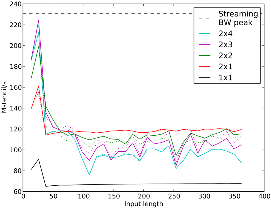
We begin our experiments with the 3-point stencil (Figure 8), the computational building block for the other experiments in our work. For a more accurate streaming bandwidth peak estimation, we considers 3.7 bytes/s read, from the DRAM, and 5.3 bytes/s write bandwidth at the stencil computations. Also, we compute the L3 bandwidth peak using 4.7 bytes/s read and 5.3 bytes/s write bandwidth at the stencil computations. The 3-point stencil has the lowest arithmetic intensity of the three stencils studied, and unlike its 7-point and 27-point cousins, does not see an increase in effective arithmetic intensity when unrolland-jam is employed. It is clear from Section 4.2 that the load-copy kernel is more efficient in bandwidth-bound situations, so we use it as the basis for our unroll-and-jam experiments. We see the strongest performance in the three problems that fit partially in the L1 cache (the peak of 224 Mstencil/s is observed at 26 3 ), with a drastic drop off as the problem inputs transition to the L3. The most robust kernel is the 2 × 1 jam, which reads and writes to two streams simultaneously, and can therefore engage the L2 prefetch unit most effectively. The larger unrolls (2 × 2, 2 × 3, and 2 × 4), enjoy greater performance in and near the L1, but then suffer drastic performance penalties as they exit the L1 and yet another performance dip near 250 3 . Disabling optimistic L2 prefetch does not seem to have any large effect on the 2 × 1 kernel, though it unreliably helps or hinders the other kernels.
The 3-point kernel seems to be an ideal target on the PowerPC 450 for standard unrolling in the fastest moving dimension, k , a technique we did not attempt due to its limited application to the larger problems we studied. Unroll-and-jam at sufficient sizes to properly cover pipeline hazards overwhelms the L2 streaming unit due to the large number of simultaneous streams to memory. Unrolling in k would cover these pipeline hazards without increasing the number of streams.
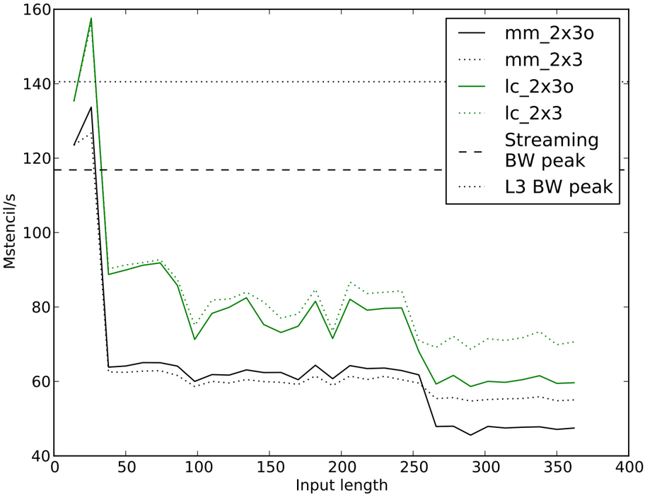
## 5.2 7-Point Stencil Computations
Our next experiment focuses on the performance of the 7-point stencil operator (Figure 9). We compare the mutate-mutate and load-copy kernels using the same unroll configurations. We note that the mutate-mutate kernel can support a slightly more aggressive unroll-andjam on this problem with a compressed usage of general purpose registers that was only implemented for the 27-point stencil.
Once again we notice strong performance within the L1, then a dropoff as the loads start coming from the L3 instead of the L1. The performance drop near 256 3 is caused when the 2 × 3 kernel's frame size of (2 + 2)(3 + 2) -4 = 16 multiplied by the length of the domain exceeds the size of L1. For smaller sizes, neighbors in the j direction can reside in L1 between consecutive passes so that only part of the input frame needs to be supplied by streams from memory. With up to 16 input streams and 2 · 3 = 6 output streams, there is no hope of
Figure 8: 3-point stencil performance with load-copy kernel at various unroll-and-jams (ixj). L3 bandwidth peak is 265 Mstencil/s
<details>
<summary>Image 6 Details</summary>
### Visual Description
## Line Chart: Performance Comparison of Different Stencil Sizes
### Overview
This image presents a line chart comparing the performance (measured in Mstencils/s) of different stencil sizes (1x1, 2x1, 2x2, 2x3, 2x4) against input length. A dashed line represents the performance of "Streaming BW peak". The chart aims to illustrate how the performance of stencil operations varies with input length and stencil size.
### Components/Axes
* **X-axis:** "Input length" ranging from 0 to 400 (units not specified, but likely characters or data points). Marked with increments of 50.
* **Y-axis:** "Mstencils/s" ranging from 60 to 240. Marked with increments of 20.
* **Legend:** Located in the top-right corner. Contains the following labels and corresponding line colors:
* "Streaming BW peak" (dashed black line)
* "2x4" (cyan line)
* "2x3" (magenta line)
* "2x2" (green line)
* "2x1" (red line)
* "1x1" (black line)
### Detailed Analysis
The chart displays six lines representing the performance of each stencil size and the streaming bandwidth peak.
* **Streaming BW peak (dashed black):** This line is approximately horizontal, maintaining a value around 225 Mstencils/s across the entire input length range. There is a slight dip around input length 300, but it quickly recovers.
* **2x4 (cyan):** This line exhibits a significant initial peak at an input length of approximately 25, reaching around 220 Mstencils/s. It then rapidly declines to around 80 Mstencils/s by an input length of 50. After that, it fluctuates between 80 and 110 Mstencils/s with some oscillations, ending around 100 Mstencils/s at input length 400.
* **2x3 (magenta):** This line starts at approximately 160 Mstencils/s at input length 0, drops to around 90 Mstencils/s by input length 50, and then fluctuates between 90 and 120 Mstencils/s with some oscillations. It ends around 110 Mstencils/s at input length 400.
* **2x2 (green):** This line begins at approximately 140 Mstencils/s, decreases to around 85 Mstencils/s by input length 50, and then fluctuates between 90 and 115 Mstencils/s. It ends around 105 Mstencils/s at input length 400.
* **2x1 (red):** This line starts at approximately 170 Mstencils/s, drops to around 110 Mstencils/s by input length 50, and then remains relatively stable between 110 and 125 Mstencils/s. It ends around 120 Mstencils/s at input length 400.
* **1x1 (black):** This line shows a sharp initial drop from approximately 150 Mstencils/s to around 70 Mstencils/s by input length 50. It then stabilizes around 110-120 Mstencils/s, with some minor fluctuations, and ends around 115 Mstencils/s at input length 400.
### Key Observations
* The "Streaming BW peak" provides a performance ceiling for all stencil sizes.
* Larger stencil sizes (2x4, 2x3, 2x2) exhibit a more pronounced initial performance drop compared to smaller stencil sizes (2x1, 1x1).
* All stencil sizes converge to a similar performance level (around 110-125 Mstencils/s) as the input length increases.
* The 1x1 stencil size shows the most stable performance after the initial drop.
### Interpretation
The data suggests that the performance of stencil operations is heavily influenced by the input length, particularly at lower lengths. Larger stencil sizes initially offer higher performance but suffer a more significant performance degradation as the input length increases. This could be due to increased memory access costs or cache misses associated with larger stencils. As the input length grows, the performance of all stencil sizes converges, indicating that the overhead associated with the stencil size becomes less significant compared to other factors, such as memory bandwidth or computational complexity. The "Streaming BW peak" represents the theoretical maximum performance achievable, and the stencil operations are all operating below this limit. The initial peak for the 2x4 stencil might indicate a benefit from increased parallelism at very small input sizes, but this benefit is quickly outweighed by the associated overhead as the input length increases. The stability of the 1x1 stencil suggests that it might be a more efficient choice for larger input lengths where performance consistency is prioritized over initial peak performance.
</details>
effectively using the L2 prefetch unit. The load-copy kernel shows better performance than the mutate-mutate kernel, as it is clear here that load/store cycles are more constrained than floating point cycles. We also notice that performance of the load-copy kernel improves with the L2 optimistic prefetch disabled slightly within the L3, and drastically when going to the DDR banks. This is likely due to the kernel's improved performance, and therefore increased sensitivity with regards to latency from the memory subsystem. It is likely that the 7-point stencil could attain better results by incorporating cache tiling strategies, though we note that without any attempts at cache tiling the performance of this result is commensurate with previously reported results for the PowerPC 450 that focused on cache tiling for performance tuning.
## 5.3 27-Point Stencil Computations
The 27-point stencil should be amenable to using a large number of jammed unrolls due to the high level of reuse between neighboring stencils. Indeed, we see nearly perfect scaling in Figure 10 as we increase the number of jams from 1 to 6 using the mutate-mutate kernel. Although there is a gradual drop off from the peak of 54 Mstencil/s (85% of arithmetic peak)
Figure 9: 7-point stencil performance comparison between mutate-mutate (mm) and loadcopy (lc) kernels at a fixed unroll-and-jam (i=2 and j=3). Experiments with L2 optimistic prefetch ends with 'o'
<details>
<summary>Image 7 Details</summary>
### Visual Description
## Line Chart: Performance Comparison of Different Configurations
### Overview
This line chart compares the performance (measured in Mstencil/s) of several configurations – `mm_2x3o`, `mm_2x3`, `lc_2x3o`, `lc_2x3`, `Streaming BW peak`, and `L3 BW peak` – across varying input lengths (ranging from 0 to 400). The chart visualizes how performance changes as the input length increases for each configuration.
### Components/Axes
* **X-axis:** Input length, ranging from approximately 0 to 400. The axis is labeled "Input length".
* **Y-axis:** Performance, measured in Mstencil/s, ranging from approximately 40 to 160. The axis is labeled "Mstencil/s".
* **Legend:** Located in the top-right corner of the chart. It identifies each line with its corresponding configuration:
* `mm_2x3o` (Black solid line)
* `mm_2x3` (Gray solid line)
* `lc_2x3o` (Green solid line)
* `lc_2x3` (Gray dotted line)
* `Streaming BW peak` (Black dashed line)
* `L3 BW peak` (Gray dotted line)
### Detailed Analysis
Here's a breakdown of each line's trend and approximate data points:
* **`mm_2x3o` (Black solid line):** Starts at approximately 60 Mstencil/s at an input length of 0, decreases sharply to around 45 Mstencil/s at an input length of 20, then gradually increases to around 65 Mstencil/s at an input length of 300, and finally drops to approximately 50 Mstencil/s at an input length of 400.
* **`mm_2x3` (Gray solid line):** Begins at approximately 55 Mstencil/s at an input length of 0, fluctuates between 60 and 75 Mstencil/s for input lengths between 20 and 250, and then decreases to around 50 Mstencil/s at an input length of 400.
* **`lc_2x3o` (Green solid line):** Exhibits a dramatic initial spike, starting at approximately 150 Mstencil/s at an input length of 0, peaking at around 155 Mstencil/s at an input length of 10, then rapidly declines to approximately 80 Mstencil/s at an input length of 50. It then fluctuates between 70 and 90 Mstencil/s for input lengths between 50 and 300, and finally decreases to around 70 Mstencil/s at an input length of 400.
* **`lc_2x3` (Gray dotted line):** Starts at approximately 140 Mstencil/s at an input length of 0, decreases to around 80 Mstencil/s at an input length of 50, and then fluctuates between 75 and 90 Mstencil/s for input lengths between 50 and 300, ending at approximately 70 Mstencil/s at an input length of 400.
* **`Streaming BW peak` (Black dashed line):** Maintains a relatively constant performance of approximately 120 Mstencil/s across all input lengths.
* **`L3 BW peak` (Gray dotted line):** Starts at approximately 125 Mstencil/s at an input length of 0, decreases to around 115 Mstencil/s at an input length of 50, and then remains relatively constant at around 120 Mstencil/s for the remainder of the input length range.
### Key Observations
* `lc_2x3o` demonstrates the most significant initial performance spike, followed by a rapid decline.
* `Streaming BW peak` and `L3 BW peak` exhibit the most stable performance across all input lengths.
* `mm_2x3o` and `mm_2x3` show similar trends, with relatively moderate performance fluctuations.
* `lc_2x3` and `lc_2x3o` have similar performance after the initial spike of `lc_2x3o`.
### Interpretation
The chart suggests that the `lc_2x3o` configuration is highly sensitive to input length, offering exceptional performance for very small inputs but quickly diminishing as the input length increases. The `Streaming BW peak` and `L3 BW peak` configurations provide consistent performance regardless of input length, making them suitable for applications requiring stable throughput. The `mm_2x3o` and `mm_2x3` configurations offer a balance between performance and stability, but their performance is generally lower than the peak performance of `lc_2x3o` for small inputs. The initial spike of `lc_2x3o` could indicate a benefit from a specific optimization that is only effective for very small input sizes. The relatively flat lines of `Streaming BW peak` and `L3 BW peak` suggest that these configurations are less affected by input size, potentially due to buffering or other mechanisms that mitigate the impact of varying input lengths. The differences between `mm` and `lc` configurations could be related to memory management or data locality strategies.
</details>
as the problem sizes increase to the point that there is little reuse from the L1 cache, the kernel consistently sustains an average of 45 Mstencil/s (70% of arithmetic peak), even when the problem sizes greatly exceed the L3 cache.
Despite the L2-overwhelming frame size ((2 + 2)(3 + 2) = 20 input streams and 2 · 3 = 6 output streams), the jammed stencil achieves good performance with no blocking largely due to the high level of reuse of input data afforded by the unrolls in i and j .
## 5.4 Model Validation
As we utilized a simulator which incorporates a model of the architecture's performance characteristics to produce our kernels, we sought to validate our performance model by comparing the implicit predictions of our generative system to the empirical results seen in Table 3.
Since performance within a core is often considerably easier to predict than when one must go beyond the core for memory access, we divide our comparisons into those on-core (L1) and those that go off the core, to L3 or main memory (streaming).
Figure 10: 27-point stencil performance with mutate-mutate kernel at various unroll-andjams (ixj). Best L3 bandwidth peak is 118 Mstencil/s and best streaming bandwidth peak is 97.5 Mstencil/s, both corresponds to 2x3 unroll-and-jam
<details>
<summary>Image 8 Details</summary>
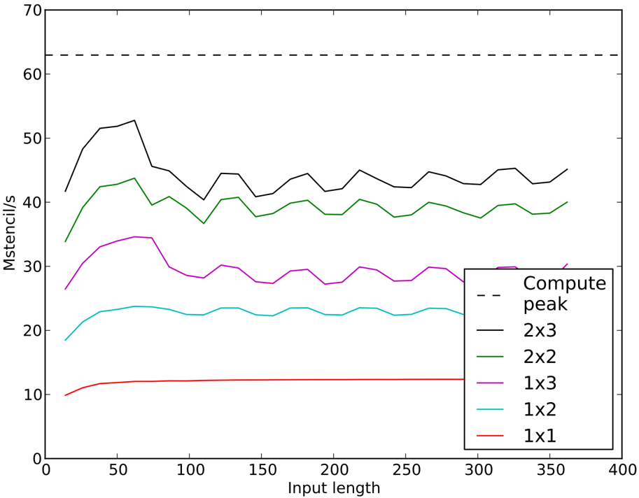
### Visual Description
\n
## Line Chart: Mstencil/s vs. Input Length
### Overview
This image presents a line chart comparing the performance (measured in Mstencil/s) of different compute peak configurations as a function of input length. The chart displays six data series, each representing a different compute peak configuration (2x3, 2x2, 1x3, 1x2, 1x1) alongside a baseline "Compute peak" performance.
### Components/Axes
* **X-axis:** "Input length" ranging from 0 to 400, with tick marks at intervals of 50.
* **Y-axis:** "Mstencil/s" ranging from 0 to 70, with tick marks at intervals of 10.
* **Legend:** Located in the bottom-right corner, listing the following data series with corresponding colors:
* Compute peak (dashed black line)
* 2x3 (black line)
* 2x2 (green line)
* 1x3 (light grey line)
* 1x2 (cyan line)
* 1x1 (red line)
### Detailed Analysis
The chart displays the performance of each configuration across the input length range.
* **Compute peak (dashed black line):** This line is horizontal and remains constant at approximately 65 Mstencil/s throughout the entire input length range.
* **2x3 (black line):** This line starts at approximately 48 Mstencil/s at an input length of 0, fluctuates between approximately 40 and 52 Mstencil/s, and ends at approximately 45 Mstencil/s at an input length of 400.
* **2x2 (green line):** This line begins at approximately 40 Mstencil/s at an input length of 0, fluctuates between approximately 35 and 45 Mstencil/s, and ends at approximately 40 Mstencil/s at an input length of 400.
* **1x3 (light grey line):** This line starts at approximately 32 Mstencil/s at an input length of 0, fluctuates between approximately 25 and 35 Mstencil/s, and ends at approximately 30 Mstencil/s at an input length of 400.
* **1x2 (cyan line):** This line begins at approximately 20 Mstencil/s at an input length of 0, increases to approximately 25 Mstencil/s around an input length of 100, and then fluctuates between approximately 20 and 25 Mstencil/s, ending at approximately 22 Mstencil/s at an input length of 400.
* **1x1 (red line):** This line remains relatively constant at approximately 10 Mstencil/s throughout the entire input length range.
### Key Observations
* The "Compute peak" configuration consistently outperforms all other configurations across all input lengths.
* The 2x3 configuration generally performs better than the 2x2, 1x3, 1x2, and 1x1 configurations.
* The 1x1 configuration exhibits the lowest performance.
* The performance of most configurations (2x3, 2x2, 1x3, 1x2) fluctuates with increasing input length, suggesting some sensitivity to input size.
### Interpretation
The data suggests that the "Compute peak" configuration provides the highest performance for this stencil operation, regardless of input length. Larger compute peak configurations (2x3, 2x2) generally offer better performance than smaller ones (1x3, 1x2, 1x1). The fluctuations in performance for the 2x3, 2x2, 1x3, and 1x2 configurations could be due to factors such as memory access patterns, cache utilization, or overhead associated with parallelization. The consistent low performance of the 1x1 configuration indicates that it is likely limited by computational resources or inefficient parallelization. The chart demonstrates the trade-offs between compute peak configuration and performance, highlighting the importance of selecting an appropriate configuration based on the specific application and input characteristics.
</details>
Our modeling of the 27-point stencils can be seen to be highly accurate in Table 3. Inside the L1 cache the disparity between predicted and actual performance is consistently less than 1%. Shifting our attention to the streaming predictions, our accuracy can be seen to be considerably degraded. This is not surprising, given that our simulator was largely targeted to model the L1 domain. However, the relative error is less than 15% in all cases; this appears to be sufficient for producing highly efficient code. This shortcoming appears to stem directly from the level of detail with which we model the shared L3 cache and main memory subsystem and we are working to address this in our simulator.
The match between predicted and witnessed performance for the 7-point stencil shows the same pattern. When modeling performance inside the L1 our relative error is less than 10%, but when extending our prediction to the components of the system shared by all four cores, our error is as great as 17.5%. Our greatest error in this instance is an underprediction that is probably attributable to a fortuitous alignment of the continuous vectors in the k-direction, as staggering these carefully often result in bandwidth benefits on the order of 10-15%.
Finally, we assess our model for the 3-point stencil. Again we see good agreement between the model and observed performance within the L1, though prediction accuracy degrades for problem sizes requiring streaming. From some further experimentation, we are reasonably certain that the chief reason for our lack of accuracy in predicting performance outside of the L1 stems from the bandwidth that must be shared between the multiple write streams and our failure to account for this in our model. It is most apparent in the 3-point stencil predictions as the ratio of write streams to either read streams or floating point operations is highest in this case.
## 6 Concluding Remarks
## 6.1 Conclusion
The main contribution of this work is effective register and instruction scheduling for constant coefficient linear operators on power-efficient processors. The loads of the input vector elements and stores of the output vector elements are minimized and the fraction of multiplyadds among all cycles is maximized. This is achieved by using two novel 3-point streamcomputation sub-kernels designed for the PowerPC 450's instruction set, mutate-mutate and load-copy. Both kernels were possible without data layout reordering because of the extensively multiplexed SIMD-like floating point units implemented in the PowerPC 450 core.
Recommendations for the research agenda for computational software libraries in the exascale domain include the the fusion of library routine implementations as well as the creation of frameworks that enable the optimal instantiation of a given routine when supplied with architectural information [13]. We feel that the work presented here is a contribution to that end. Further, the nature of our simulator allows us to optimize our code as measured by other metrics such as bandwidth or energy consumption, given a simple model of the cost. We also demonstrate performance comparable to advanced cache tiling approaches for the 7-point stencil, despite the fact that we make no effort to optimize for cache reuse.
## 6.2 Future Work
While the three problems considered (3-point stencils in one dimension and 7-point and 27-point stencils in three dimensions, with constant coefficients and symmetry within each spatial dimension, but not across them) are heavily used in applications, there are numerous generalizations. The suitability of our approach can be characterized by the arithmetic intensity associated with each generalization. We elaborate on two that tend to increase the arithmetic intensity, higher-order stencils and chained iterative passes over the vectors, and two that tend to decrease arithmetic intensity, irregular stencils and spatial varying coefficients.
Higher-order stencils expand the number of adjacent input vector elements that enter into a single output vector element, in successive steps of semi-width one in each of the spatial dimensions i , j , and k , with an additional weight coefficient corresponding to each additional increment of semi-width in each dimension. This is a modest generalization. Higher-order
Table 3: Predictions vs. observations for in-L1 and streaming performance, in Megastencils per second
| 3-lc-2x4 | 3-lc-2x3 | 3-lc-2x2 | 3-lc-2x1 | 3-lc-1x1 | 7-lc-2x3 | 7-mm-2x3 | 27-mm-2x3 | 27-mm-2x2 | 27-mm-1x3 | 27-mm-1x2 | 27-mm-1x1 | Kernel |
|------------|------------|------------|------------|------------|------------|------------|-------------|-------------|-------------|-------------|-------------|---------------------|
| 425 | 425 | 425 | 425 | 425 | 212.5 | 182.14 | 62.96 | 62.96 | 62.96 | 62.96 | 44.74 | Instruction Naive |
| 197.1 | 202.31 | 193.36 | 147.29 | 88.12 | 143.83 | 126.84 | 54.62 | 44.59 | 34.3 | 23.35 | 11.93 | limits Simulated |
| 338.72 | 338.72 | 338.72 | 338.72 | 338.72 | 203.54 | 203.54 | 175.52 | 154.28 | 130.58 | 113.19 | 80.88 | Bandwidth L1 |
| 231.51 | 231.51 | 231.51 | 231.51 | 231.51 | 116.84 | 116.84 | 97.51 | 83.68 | 68.99 | 58.69 | 40.54 | limits streaming |
| 197.1 | 202.31 | 193.36 | 147.29 | 88.12 | 143.83 | 126.84 | 54.62 | 44.59 | 34.3 | 23.35 | 11.93 | In-L1 Predicted |
| 199.05 | 195.83 | 184.84 | 142.04 | 81.33 | 132.1 | 124.43 | 54.17 | 44.53 | 34.23 | 23.39 | 11.92 | Observed |
| 197.1 | 202.31 | 193.36 | 147.29 | 88.12 | 116.84 | 116.84 | 54.62 | 44.59 | 34.3 | 23.35 | 11.93 | Streaming Predicted |
| 83.9 | 86.62 | 96.23 | 119.99 | 67.44 | 74.21 | 59.69 | 42.64 | 38.37 | 28.26 | 22.56 | 12.37 | Observed |
discretization increases register pressure because of the larger number of inputs that combine in each output. Opportunities for reuse of input elements expand with the stencil width up to the ability to keep them resident. In a P -point regular stencil (regardless of number of spatial dimensions) each input element is operated upon with a pre-stored weight P times: once in the stencil centered upon it, and once in each neighboring stencil with which its own stencil overlaps. Floating point arithmetic intensity increases in proportion to P . That is, if there are N elements in the input or output array, there are PN floating point multiply-adds per N floating reads and N floating writes. Explicit methods for nonlinear systems, especially with high-order discretization techniques such as Weighted Essentially Non-Oscillatory (WENO) or discontinuous Galerkin [36], have similar properties, including a larger number of input streams, but with much higher arithmetic intensity.
S -stage chaining (as in the simultaneous accumulation of Ax , A 2 x , A 3 x , . . . A s x ) allows the output vector to be fed back as input before being written. Per output vector of N floating point writes, there are N/S reads and PN floating point multiply-adds. Therefore, up to the ability to keep the additional operands cached, both higher-order operators and chained operations improve the potential for the transformations described here.
Irregular stencils require integer reads, in addition to floating point reads to determine which elements of the input vector go with each row of the matrix. This further dilutes advantages that lead to the great breakthroughs in stencils per second described here. Stencil operations with constant coefficients and sparse matrix-vector multiplies with general coefficients are similar when counting floating operations, but very different when it comes to data volume.
Spatially varying coefficients require the loading of additional weights, each of which is used only once, each of which is of the same floating precision of the input and output vectors, P of them in the production of each output vector element, with each input vector element being combined with P different weights. While each input and output element can still be reused up to P times in the execution of one pass through the overall vector-to-vector map, the dominant array in the workspace is the coefficient matrix of weights so the benefits of reusing the vectors are minimal. This situation is typical for nonlinear problems when using Newton-Krylov and linear multigrid methods. However, when 'free flops' are available, the weights can also be recomputed on the fly as a nonlinear function of a given state and/or scalar coefficients. In this case, the number of input streams is similar to the linear constant coefficient case (perhaps larger by a factor of 2 or 3), but the number of floating point results is several times higher and involves the problem-specific 'physics.' Putting the physics inside the kernel like this suggests that there will be an emphasis on the ability to quickly develop high-performance kernels for new physics.
## Acknowledgments
We are grateful to Andy Ray Terrel for his helpful commentary on an early draft of this paper. We are also indebted to Andrew Winfer for his support in conducting our numerical experiments on the Shaheen Blue Gene/P system at the KAUST Supercomputing Laboratory, and to Vernon Austel for his assistance in running experiments on the Blue Gene/P system at IBM's Watson Research Center.
## References
- [1] Rajagopal Ananthanarayanan, Steven K Esser, Horst D Simon, and Dharmendra S Modha. The cat is out of the bag: cortical simulations with 109 neurons, 1013 synapses. In Proceedings of the Conference on High Performance Computing Networking, Storage and Analysis , SC '09, pages 63:1--63:12, New York, NY, USA, 2009. ACM.
- [2] Mauricio Araya-Polo, F´ elix Rubio, Ra´ ul De, Mauricio Hanzich, and Jos´ e Mar´ ıa. 3D seismic imaging through reverse-time migration on homogeneous and heterogeneous multi-core processors. Scientific Programming , 17:185-198, 2009.
- [3] D.H. Bailey, E. Barszcz, J.T. Barton, D.S. Browning, R.L. Carter, L. Dagum, R.A. Fatoohi, P.O. Frederickson, T.A. Lasinski, R.S. Schreiber, H.D. Simon, V. Venkatakrishnan, and S.K. Weeratunga. The NAS parallel benchmarks. International Journal of High Performance Computing Applications , 5(3):63, 1991.
- [4] MJ Berger and J Oliger. Adaptive Mesh Refinement for Hyperbolic Partial Differential Equations. Journal of Computational Physics , 53(3):484-512, 1984.
- [5] D. Callahan, J. Cocke, and K. Kennedy. Estimating interlock and improving balance for pipelined architectures 1. Journal of Parallel and Distributed Computing , 5(4):334-358, 1988.
- [6] S. Carr and K. Kennedy. Improving the ratio of memory operations to floatingpoint operations in loops. ACM Transactions on Programming Languages and Systems (TOPLAS) , 16(6):1768-1810, 1994.
- [7] C.M. Chang, C.M. Chen, and C.T. King. Using integer linear programming for instruction scheduling and register allocation in multi-issue processors 1. Computers & Mathematics with Applications , 34(9):1-14, 1997.
- [8] Matthias Christen, Olaf Schenk, and Helmar Burkhart. Automatic code generation and tuning for stencil kernels on modern shared memory architectures. Computer Science Research and Development , 26(3-4):205-210, April 2011.
- [9] Matthias Christen, Olaf Schenk, Esra Neufeld, Peter Messmer, and Helmar Burkhart. Parallel data-locality aware stencil computations on modern micro-architectures. In 2009 IEEE International Symposium on Parallel & Distributed Processing , pages 1-10. IEEE, May 2009.
- [10] Dac C. Pham, Tony Aipperspach, David Boerstler, Mark Bolliger, Rajat Chaudhry, Dennis Cox, Paul Harvey, Paul M. Harvey, H. Peter Hofstee, Charles Johns, Jim Kahle, Atsushi Kameyama, John Keaty, Yoshio Masubuchi, Mydung Pham, J¨ urgen Pille, Stephen Posluszn, Kazuaki Yazawa. Overview of the architecture, circuit design, and physical implementation of a first-generation cell processor. Solid-State Circuits, IEEE Journal of , 41(1):179-196, 2006.
- [11] K. Datta, S. Williams, V. Volkov, J. Carter, L. Oliker, J. Shalf, and K. Yelick. Autotuning the 27-point Stencil for Multicore. In Proc. iWAPT2009: The Fourth International Workshop on Automatic Performance Tuning , 2009.
- [12] Kaushik Datta. Auto-tuning Stencil Codes for Cache-Based Multicore Platforms . PhD thesis, EECS Department, University of California, Berkeley, December 2009.
- [13] Jack Dongarra, Pete Beckman, Terry Moore, Patrick Aerts, Giovanni Aloisio, JeanClaude Andre, David Barkai, Jean-Yves Berthou, Taisuke Boku, Bertrand Braunschweig, Franck Cappello, Barbara Chapman, Chi Xuebin, Alok Choudhary, Sudip Dosanjh, Thom Dunning, Sandro Fiore, Al Geist, William Gropp, Robert Harrison, Mark Hereld, Michael Heroux, Adolfy Hoisie, Koh Hotta, Jin Zhong, Yutaka Ishikawa, Fred Johnson, Sanjay Kale, Richard Kenway, David Keyes, Bill Kramer, Jesus Labarta, Alain Lichnewsky, Thomas Lippert, Bob Lucas, Barney Maccabe, Satoshi Matsuoka, Paul Messina, Peter Michielse, Bernd Mohr, Matthias S. Mueller, Wolfgang E. Nagel, Hiroshi Nakashima, Michael E Papka, Dan Reed, Mitsuhisa Sato, Ed Seidel, John Shalf, David Skinner, Marc Snir, Thomas Sterling, Rick Stevens, Fred Streitz, Bob Sugar, Shinji Sumimoto, William Tang, John Taylor, Rajeev Thakur, Anne Trefethen, Mateo Valero, Aad van der Steen, Jeffrey Vetter, Peg Williams, Robert Wisniewski, and Kathy Yelick. The international exascale software project roadmap. International Journal of High Performance Computing Applications , 25(1):3-60, 2011.
- [14] Hikmet Dursun, Ken-Ichi Nomura, Liu Peng, Richard Seymour, Weiqiang Wang, Rajiv K Kalia, Aiichiro Nakano, and Priya Vashishta. A Multilevel Parallelization Framework for High-Order Stencil Computations. In Proceedings of the 15th International Euro-Par Conference on Parallel Processing , Euro-Par '09, pages 642-653, Berlin, Heidelberg, 2009. Springer-Verlag.
- [15] A.E. Eichenberger, P. Wu, and K. O'Brien. Vectorization for SIMD architectures with alignment constraints. ACM SIGPLAN Notices , 39(6):82-93, 2004.
- [16] W. Feng and K. Cameron. The Green500 List: Encouraging Sustainable Supercomputing. COMPUTER , pages 50-55, 2007.
- [17] A. Ganapathi, K. Datta, A. Fox, and D. Patterson. A case for machine learning to optimize multicore performance. In Proceedings of the First USENIX conference on Hot topics in parallelism , pages 1-1. USENIX Association, 2009.
- [18] Amol Ghoting and Konstantin Makarychev. Indexing genomic sequences on the IBM Blue Gene. In Proceedings of the Conference on High Performance Computing Networking, Storage and Analysis , SC '09, pages 61:1--61:11, New York, NY, USA, 2009. ACM.
- [19] John L Hennessy and Thomas Gross. Postpass Code Optimization of Pipeline Constraints. ACM Trans Program Lang Syst , 5(3):422-448, 1983.
- [20] T. Henretty, K. Stock, L.N. Pouchet, F. Franchetti, J. Ramanujam, and P. Sadayappan. Data Layout Transformation for Stencil Computations on Short-Vector SIMD Architectures. In Compiler Construction , pages 225-245. Springer, 2011.
- [21] IBM Blue Gene Team. Overview of the IBM Blue Gene/P project. IBM J. Res. Dev. , 52(1/2):199--220, 2008.
- [22] S. Kamil, C. Chan, L. Oliker, J. Shalf, and S. Williams. An auto-tuning framework for parallel multicore stencil computations. In Parallel & Distributed Processing (IPDPS), 2010 IEEE International Symposium on , pages 1-12. IEEE, 2010.
- [23] Shoaib Kamil, Kaushik Datta, Samuel Williams, Leonid Oliker, John Shalf, and Katherine Yelick. Implicit and explicit optimizations for stencil computations. Proceedings of the 2006 workshop on Memory system performance and correctness - MSPC '06 , page 51, 2006.
- [24] Shoaib Kamil, Parry Husbands, Leonid Oliker, John Shalf, and Katherine Yelick. Impact of modern memory subsystems on cache optimizations for stencil computations. Memory System Performance , pages 36-43, 2005.
- [25] D.E. Keyes. Exaflop/s: The why and the how. Comptes Rendus M´ ecanique , 339(23):70-77, 2011.
- [26] Sriram Krishnamoorthy, Muthu Baskaran, Uday Bondhugula, J Ramanujam, Atanas Rountev, and P Sadayappan. Effective automatic parallelization of stencil computations. ACM Sigplan Notices , 42(6):235, 2007.
- [27] Pat Hanrahan Larry Seiler, Doug Carmean, Eric Sprangle, Tom Forsyth, Michael Abrash, Pradeep Dubey, Stephen Junkins, Adam Lake, Jeremy Sugerman, Robert Cavin, Roger Espasa, Ed Grochowski, Toni Juan. Larrabee: a many-core x86 architecture for visual computing. In ACM SIGGRAPH 2008 papers , pages 1-15. ACM, 2008.
- [28] Z. Li and Y. Song. Automatic tiling of iterative stencil loops. ACM Transactions on Programming Languages and Systems (TOPLAS) , 26(6):975-1028, 2004.
- [29] E. Lindholm, J. Nickolls, S. Oberman, and J. Montrym. NVIDIA Tesla: A unified graphics and computing architecture. Micro, IEEE , 28(2):39-55, 2008.
- [30] C Mueller and B Martin. CorePy: High-Productivity Cell/BE Programming. Applications for the Cell/BE , 2007.
- [31] C.J. Newburn, B. So, Z. Liu, M. McCool, A. Ghuloum, S. Du Toit, Z.G. Wang, Z.H. Du, Y. Chen, G. Wu, Peng Guo, Zhanglin Liu, and Dan Zhang. Intel's Array Building Blocks: A Retargetable, Dynamic Compiler and Embedded Language. Proceedings of Code Generation and Optimization , 2011.
- [32] A. Nguyen, N. Satish, J. Chhugani, C. Kim, and P. Dubey. 3.5-D Blocking Optimization for Stencil Computations on Modern CPUs and GPUs. sc , pages 1-13, 2010.
- [33] Liu Peng, Richard Seymour, Ken-Ichi Nomura, R K Kalia, Aiichiro Nakano, P Vashishta, Alexander Loddoch, Michael Netzband, W R Volz, and C C Wong. Highorder stencil computations on multicore clusters. IPDPS , pages 1-11, 2009.
- [34] D F Richards, J N Glosli, B Chan, M R Dorr, E W Draeger, J.-L. Fattebert, W D Krauss, T Spelce, F H Streitz, M P Surh, and J A Gunnels. Beyond homogeneous decomposition: scaling long-range forces on Massively Parallel Systems. In Proceedings of the Conference on High Performance Computing Networking, Storage and Analysis , SC '09, pages 60:1--60:12, New York, NY, USA, 2009. ACM.
- [35] Gabriel Rivera and C W Tseng. Tiling optimizations for 3D scientific computations. In Proceedings of SC00 . IEEE Computer Society, 2000.
- [36] C.W. Shu. High-order finite difference and finite volume WENO schemes and discontinuous Galerkin methods for CFD. International Journal of Computational Fluid Dynamics , 17(2):107-118, 2003.
- [37] A. Solar-Lezama, G. Arnold, L. Tancau, R. Bodik, V. Saraswat, and S. Seshia. Sketching stencils. In Proceedings of the 2007 ACM SIGPLAN conference on Programming language design and implementation , pages 167-178. ACM, 2007.
- [38] Sosa, C. and International Business Machines Corporation Organization. International Technical Support. IBM system Blue Gene solution: Blue Gene/P application development . IBM International Technical Support Organization, 2008.
- [39] Yuan Tang, Rezaul Alam Chowdhury, Bradley C. Kuszmaul, Chi-Keung Luk, and Charles E. Leiserson. The pochoir stencil compiler. In Proceedings of the 23rd ACM symposium on Parallelism in algorithms and architectures - SPAA '11 , page 117, New York, New York, USA, June 2011. ACM Press.
- [40] Gerhard Wellein, Georg Hager, Thomas Zeiser, Markus Wittmann, and Holger Fehske. Efficient Temporal Blocking for Stencil Computations by Multicore-Aware Wavefront Parallelization. 2009 33rd Annual IEEE International Computer Software and Applications Conference , pages 579-586, 2009.
- [41] K Wilken. Optimal instruction scheduling using integer programming. ACM SIGPLAN Notices , 2000.
- [42] Samuel Williams, Jonathan Carter, Leonid Oliker, John Shalf, and Katherine Yelick. Lattice Boltzmann simulation optimization on leading multicore platforms. 2008 IEEE International Symposium on Parallel and Distributed Processing , 69(9):1-14, 2008.