# Unknown Title
## QUANTUM ANNEALING: FROM VIEWPOINTS OF STATISTICAL PHYSICS, CONDENSED MATTER PHYSICS, AND COMPUTATIONAL PHYSICS
## SHU TANAKA
Department of Chemistry, University of Tokyo, 7-3-1, Hongo, Bunkyo-ku, Tokyo, 113-0033, Japan E-mail: shu-t@chem.s.u-tokyo.ac.jp
## RYO TAMURA
Institute for Solid State Physics, University of Tokyo, 5-1-5, Kashiwanoha, Kashiwa-shi, Chiba, 277-8501, Japan
International Center for Young Scientists, National Institute for Materials Science, 1-2-1, Sengen, Tsukuba-shi, Ibaraki, 305-0047, Japan E-mail: tamura.ryo@nims.go.jp
In this paper, we review some features of quantum annealing and related topics from viewpoints of statistical physics, condensed matter physics, and computational physics. We can obtain a better solution of optimization problems in many cases by using the quantum annealing. Actually the efficiency of the quantum annealing has been demonstrated for problems based on statistical physics. Then the quantum annealing has been expected to be an efficient and generic solver of optimization problems. Since many implementation methods of the quantum annealing have been developed and will be proposed in the future, theoretical frameworks of wide area of science and experimental technologies will be evolved through studies of the quantum annealing.
Keywords : Quantum annealing; Quantum information; Ising model; Optimization problem
## 1. Introduction
Optimization problems are present almost everywhere, for example, designing of integrated circuit, staff assignment, and selection of a mode of transportation. To find the best solution of optimization problems is difficult in general. Then, it is a significant issue to propose and to develop a method for obtaining the best solution (or a better solution) of optimiza-
tion problems in information science. In order to obtain the best solution, a couple of algorithms according to type of optimization problems have been formulated in information science and these methods have yielded practical applications. Furthermore, since optimization problem is to find the state where a real-valued function takes the minimum value, it can be regarded as problem to obtain the ground state of the corresponding Hamiltonian. Thus, if we can map optimization problem to well-defined Hamiltonian, we can use knowledge and methodologies of physics. Actually, in computational physics, generic and powerful algorithms which can be adopted for wide application have been proposed. One of famous methods is simulated annealing which was proposed by Kirkpatrick et al. 1,2 In the simulated annealing, we introduce a temperature (thermal fluctuation) in the considered optimization problems. We can obtain a better solution of the optimization problem by decreasing temperature gradually since thermal fluctuation effect facilitates transition between states. It is guaranteed that we can obtain the best solution definitely if we decrease temperature slow enough. 3 Then, the simulated annealing has been used in many cases because of easy implementation and guaranty.
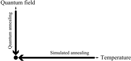
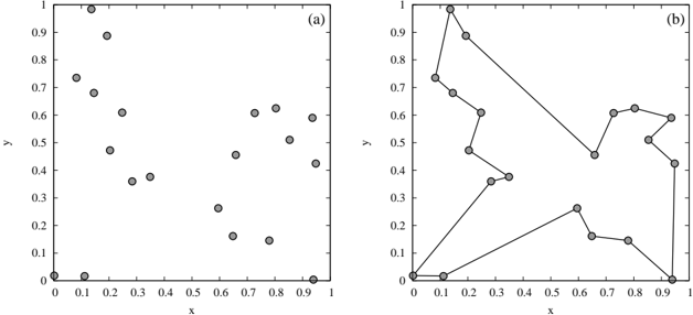
The quantum annealing was proposed as an alternative method of the simulated annealing. 4-11 In the quantum annealing, we introduce a quantum field which is appropriate for the considered Hamiltonian. For instance, if the considered optimization problem can be mapped onto the Ising model, the simplest form of the quantum fluctuation is transverse field. In the quantum annealing, we gradually decrease quantum field (quantum fluctuation) instead of temperature (thermal fluctuation). The efficiency of the quantum annealing has been demonstrated by a number of researchers, and it has been reported that a better solution can be obtained by the quantum annealing comparison with the simulated annealing in many cases. Figure 1 shows schematic picture of the simulated annealing and the quantum annealing. In optimization problems, our target is to obtain the stable state at zero temperature and zero quantum field, which is indicated by the solid circle in Fig. 1.
Recently, methods in which we decrease temperature and quantum field simultaneously have been proposed and as a result, we can obtain a better solution than the simulated annealing and the simple quantum annealing. 12-14 Moreover, as an another example of methods in which we use both thermal fluctuation and quantum fluctuation, novel quantum annealing method with the Jarzynski equality 15,16 was also proposed, 17 which is based on nonequilibrium statistical physics.
Fig. 1. Schematic picture of the simulated annealing and the quantum annealing. Our purpose is to obtain the ground state at the point indicated by the solid circle.
<details>
<summary>Image 1 Details</summary>
### Visual Description
\n
## Diagram: Annealing Landscape
### Overview
The image is a 2D diagram illustrating the relationship between temperature and annealing methods – Quantum Annealing and Simulated Annealing. It depicts a conceptual space where these methods operate, with temperature on the horizontal axis and the degree of annealing on the vertical axis. A single data point is shown in the bottom-left corner.
### Components/Axes
* **X-axis:** Labeled "Temperature", with an arrow indicating increasing temperature to the right.
* **Y-axis:** Labeled "Quantum annealing" at the top and "Quantum field" at the bottom, with an arrow indicating increasing annealing to the top.
* **Annotation:** "Simulated annealing" is written along the positive x-axis.
* **Data Point:** A filled black circle is located at the origin (approximately (0,0)).
### Detailed Analysis
The diagram shows a coordinate system with two axes representing temperature and annealing. The x-axis, labeled "Temperature", extends horizontally to the right, indicating increasing temperature. The y-axis, labeled "Quantum annealing" at the top and "Quantum field" at the bottom, extends vertically upwards, indicating increasing annealing. The annotation "Simulated annealing" is placed along the positive x-axis.
A single black circle is positioned at the origin of the coordinate system. This point represents a state of low temperature and low annealing. There are no other data points or curves present in the diagram.
### Key Observations
The diagram is highly conceptual and lacks quantitative data. The single data point suggests a starting point or a specific condition within the annealing landscape. The placement of "Simulated annealing" along the x-axis implies that it operates at varying temperatures. The diagram does not show any relationship between the two annealing methods.
### Interpretation
The diagram illustrates a conceptual space for understanding annealing processes. The x-axis represents the temperature parameter, while the y-axis represents the degree of annealing. The diagram suggests that simulated annealing operates across a range of temperatures, while the single point indicates a specific state for quantum annealing. The diagram is a simplified representation and does not provide detailed information about the behavior of these methods. It appears to be a qualitative illustration of the parameter space rather than a quantitative analysis of annealing performance. The absence of curves or additional data points limits the ability to draw more specific conclusions. The diagram is likely intended to provide a high-level overview of the relationship between temperature and annealing methods, rather than a precise depiction of their behavior.
</details>
In this paper, we review the quantum annealing method which is the generic and powerful tool for obtaining the best solution of optimization problems from viewpoints of statistical physics, condensed matter physics, and computational physics. The organization of this paper is as follows. In Sec. 2, we review the Ising model which is a fundamental model of magnetic systems. The realization method of the Ising model by nuclear magnetic resonance is also explained. In Sec. 3, we show a couple of implementation methods of the quantum annealing. In Sec. 4, we explain two optimization problems - traveling salesman problem and clustering problem. The quantum annealing based on the Monte Carlo method for the traveling salesman problem is also demonstrated. In Sec. 5, we review related topics of the quantum annealing - Kibble-Zurek mechanism of the Ising spin chain and order by disorder in frustrated systems. In Sec. 6, we summarize this paper briefly and give some future perspectives of the quantum annealing.
## 2. Ising Model
In this section we introduce the Ising model which is a fundamental model in statistical physics. A century ago, the Ising model was proposed to explain cooperative nature in strongly correlated magnetic systems from a microscopic viewpoint. 18 The Hamiltonian of the Ising model is given by
$$H _ { 1 } = - \sum _ { i , j } J _ { ij } o _ { i z } o _ { j z } - \sum _ { i = 1 } ^ { N } h _ { i }$$
where the summation of the first term runs over all interactions on the defined graph and N represents the number of spins. If the sign of J ij is positive/negative, the interaction is called ferromagnetic/antiferromagnetic
interaction. Spins which are connected by ferromagnetic/antiferromagnetic interaction tend to be the same/opposite direction. The second term of the Hamiltonian denotes the site-dependent longitudinal magnetic fields. Although the Ising model is quite simple, this model exhibits inherent rich properties e.g. phase transition and dynamical behavior such as melting process and slow relaxation. For instance, the ferromagnetic Ising model with homogeneous interaction ( J ij = J for ∀ i, j ) and no external magnetic fields ( h i = 0 for ∀ i ) on square lattice exhibits the second-order phase transition, whereas no phase transition occurs in the Ising model on onedimensional lattice. Onsager first succeeded to obtain explicitly free energy of the Ising model without external magnetic field on square lattice. 19 After that, a couple of calculation methods were proposed. Furthermore, these calculation methods have been improved day by day, and the new techniques which were developed in these methods have been applied for other more complicated problems. Since the Ising model is quite simple, we can easily generalize the Ising model in diverse ways such as the Blume-Capel model, 20,21 the clock model, 22,23 and the Potts model. 24,25 By analyzing these models, relation between nature of phase transition and the symmetry which breaks at the transition point has been investigated. Then, it is not too much to say that the Ising model has opened up a new horizon for statistical physics.
The Ising model can be adopted for not only magnetic systems but also systems in wide area of science such as information science. Optimization problem is one of important topics in information science. As we mention in Sec. 4, optimization problem can be mapped onto the Ising model and its generalized models in many cases. Then some methods which were developed in statistical physics often have been used for optimization problem. In Sec. 2.1, we show a couple of magnetic systems which can be well represented by the Ising model. In Sec. 2.2, we review how to create the Ising model by Nuclear Magnetic Resonance (NMR) technique as an example of experimental realization of the Ising model.
## 2.1. Magnetic Systems
In many cases, the Hamiltonian of magnetic systems without external magnetic field is given by
$$\hat { H } = - \sum _ { i , j } J _ { ij } ( \sigma ^ { i } _ { j } \cdot \sigma ^ { j } _ { i } )$$
where ˆ σ α i denotes the α -component of the Pauli matrix at the i -th site. The form of this interaction is called Heisenberg interaction. The definitions of Pauli matrices are
$$\sigma ^ { x } = ( 0 , 1 ) , \sigma ^ { y } = ( 0 - i , 0 )$$
where the bases are defined by
$$\begin{array}{c}
n = \left\{ 0 \right\}, \\
1 \geq n = \left\{ 1 \right\}, \\
1 + = \left\{ 4 \right\}.
\end{array}$$
In this case, magnetic interactions are isotropic. However, they become anisotropic depending on the surrounded ions in real magnetic materials. In general, the Hamiltonian of magnetic systems should be replaced by
$$a ^ { i } - \sum _ { i , j } J _ { i , j } ( c x _ { i } ^ { 2 } o ^ { 2 } f _ { j } + c y _ { i } ^ { 2 } o ^ { 2 } f _ { j } )$$
When | c x | , | c y | > | c z | , the xy -plane is easy-plane and the Hamiltonian becomes XY-like Hamiltonian. On the contrary, when | c z | > | c x | , | c y | , the z -axis is easy-axis and the Hamiltonian becomes Ising-like Hamiltonian. Such anisotropy comes from crystal structure, spin-orbit coupling, and dipoledipole coupling. Moreover, even if there is almost no anisotropy in magnetic interactions, magnetic systems can be regarded as the Ising model when the number of electrons in the magnetic ion is odd and the total spin is halfinteger. In this case, doubly degenerated states exist because of the Kramers theorem. These states are called the Kramers doublet. When the energy difference between the ground states and the first-excited states ∆ E is large enough, these doubly-degenerated ground states can be well represented by the S = 1 / 2 Ising spins. Table 1 shows examples of the magnetic materials which can be well represented by the Ising model on one-dimensional chain, two-dimensional square lattice, and three-dimensional cubic lattice.
Table 1. Examples of magnetic materials which can be represented by the Ising model on chain (one-dimension), square lattice (two-dimension), and cubic lattice (three-dimension).
| Material | Spatial dimension | Total spin | Type of interaction | J/k B | References |
|-------------------------------|---------------------|--------------|-----------------------|-------------|--------------|
| K 3 Fe(CN) 6 | One (chain) | 1 2 | Antiferromagnetic | - 0 . 23 K | 26-28 |
| CsCoCl 3 | One (chain) | 1 2 | Antiferromagnetic | - 100 K | 29,30 |
| Dy(C 2 H 5 SO 4 ) 2 · 9 H 2 O | One (chain) | 1 2 | Ferromagnetic | 0 . 2 K | 31-33 |
| CoCl 2 · 2NC 5 H 5 | One (chain) | 1 2 | Ferromagnetic | 9 . 5 K | 34,35 |
| CoCs 3 Br 5 | Two (square) | 1 2 | Antiferromagnetic | - 0 . 23 K | 36-38 |
| Co(HCOO) 2 · 2 H 2 O | Two (square) | 1 2 | Antiferromagnetic | - 4 . 3 K | 39-42 |
| Rb 2 CoF 4 | Two (square) | 1 2 | Antiferromagnetic | - 91 K | 43,44 |
| FeCl 2 | Two (square) | 1 | Ferromagnetic | 3 . 4 K | 45,46 |
| DyPO 4 | Three (cubic) | 1 2 | Antiferromagnetic | - 2 . 5 K | 47-50 |
| Dy 3 Al 5 O 12 | Three (cubic) | 1 2 | Antiferromagnetic | - 1 . 85 K | 51-53 |
| CoRb 3 Cl 5 | Three (cubic) | 1 2 | Antiferromagnetic | - 0 . 511 K | 54,55 |
| FeF 2 | Three (cubic) | 2 | Antiferromagnetic | - 2 . 69 K | 56-59 |
## 2.2. Nuclear Magnetic Resonance
In condensed matter physics, Nuclear Magnetic Resonance (NMR) has been used for decision of the structure of organic compounds and for analysis of the state in materials by using resonance induced by electromagnetic wave. The NMR can create the Ising model with transverse fields, which is expected to become an element of quantum information processing. In this processing, we use molecules where the coherence times are long compared with typical gate operations. Actually a couple of molecules which have nuclear spins were used for demonstration of quantum computing. 60-75 In this section we explain how to create the Ising model by NMR.
The setup of the NMR spectrometer as a tool of quantum computing is as follows. We first put molecules which contain nuclear spins under the strong magnetic field B 0 . Next we apply radio frequency ω (rf) magnetic field which is perpendicular to the strong magnetic field B 0 . For simplicity, we here consider a molecule which contains two spins. We also assume that the considered molecule can be well described by the Heisenberg Hamiltonian. Then the Hamiltonian of this system is given by
$$\frac { \hat { H } } { 6 } = \hat { H } _ { m o l } + \hat { H } _ { 1 ^ { r t } } + \hat { H } _ { 2 ^ { r f } }$$
where ˆ H mol , ˆ H (rf) 1 , and ˆ H (rf) 2 are defined by
$$\sigma _ { 2 } + \sigma _ { 1 } \cdot \sigma _ { 2 } + \sigma _ { 1 } \cdot \sigma _ { 3 } , ( 7 )$$
$$\frac { 1 } { 2 } ( t ) = - I _ { 2 } \cos ( w ( t ) + \phi _ { 2 } ) ( r ^ { 2 } )$$
$$\gamma ( t ) = - I _ { 1 } \cos ( w ( t ) + \phi _ { 1 } ( t ^ { 2 } )$$
respectively. We take the natural unit in which /planckover2pi1 = 1. The values of φ 1 and φ 2 are the phases at the time t = 0 of the first spin and that of the second spin, respectively. The quantities of h i are defined by h i := γ i B 0 , where γ i denotes the gyromagnetic ratio of the i -th spin ( i = 1 , 2). The values of h 1 and h 2 represent energy differences between |↑〉 and |↓〉 of the first spin and the second spin, respectively. The coefficients Γ 1 and Γ 2 in ˆ H (rf) 1 and ˆ H (rf) 2 are the effective amplitudes of the ac magnetic field, whose definitions are Γ i := γ i B ac , where B ac is amplitude of the ac magnetic field. The value of γ ′ is defined by the ratio of the gyromagnetic ratios γ ′ := γ 2 /γ 1 .
We define the following unitary transformation:
$$\int ( R ) : = e ^ { - i h _ { 1 } \phi _ { 1 } t } . e ^ { - i h _ { 2 } \phi _ { 2 } t }$$
We can change from the laboratory frame to a frame rotating with h i around the z -axis by using the above unitary transformation. The dynamics of a
density matrix can be calculated by
$$\frac { i \phi } { d t } = [ H , \phi ].$$
The density matrix on the rotating frame is given by
$$\rho ^ { ( R ) } : = U ^ { ( R ) } \dot { p } U ^ { ( R ) } t .$$
To be the same form as Eq. (11) on the rotating frame, the Hamiltonian on the rotating frame should be
$$\frac { \hat { U } ( R ) } { d t } = \hat { U } ( R ) \hat { H } U ^ { \prime } ( R ) + - i \hat { U } ^ { \prime } ( R )$$
Here we decompose the Hamiltonian on the rotating frame as
$$\frac { h ( R ) } { 2 } = \frac { h _ { mol } ( R ) } { 2 } + \frac { h _ { 1 } ( R ) ( f ) } { 2 } + r$$
where the three terms are defined by
$$\frac { H ( R ) } { \frac { d U ^ { \prime } ( R ) t } { d t } } , ( 1 5 )$$
$$\sum _ { i = 1 } ^ { n } \frac { 1 } { n } H _ { i } ( R ) = \sum _ { i = 1 } ^ { n } \frac { 1 } { n } H _ { i } ( t ) \tilde { H } ( R + t )$$
$$H _ { 2 } ^ { ( R ) ( r f ) } = \bar { U } ( R ) H _ { 2 } ^ { ( R ) ( r f ) } U ( R + t ) .$$
The intramolecular magnetic interaction Hamiltonian on the rotating frame ˆ H (R) mol can be calculated as
$$\hat { r } ( R ) = J \left\{ \begin{array}{ll} 0 & 0 & 0 \\ 0 & e ^ { - i ( h _ { 2 } - h _ { 1 } ) t } & 0 \\ 0 & 0 & 0 \end{array} \right.$$
The approximation is valid when | h 2 -h 1 | τ /greatermuch 1, where τ is a characteristic time scale since the exponential terms are averaged to vanish. The radio frequency magnetic field Hamiltonian on the rotating frame ˆ H (R)(rf) 1 under the resonance condition ω (rf) = h i can be calculated as
$$\begin{array}{ll}
\eta _ { 1 } ( R ) ( r ) = - \Gamma _ { 1 } \left[ \left\{ \begin{array}{l}
0 & 0 & e^{-i \theta _ { 1 } } \\
0 & 0 & 0 \\
e^{i \theta _ { 1 } } & 0 & 0 \\
0 & 0 & e^{i \theta _ { 1 } }
\end{array} \right. \right]
,
where a_{-1} := e^{-i ( h _ { 2 } - h ) t + \phi _ { 1 } } + e^{-i \theta _ { 1 } } .
\end{array}$$
$$\rho ^ { 1 } ( R ) ( r f ) = - \Gamma _ { 1 } ( \cos \phi _ { 1 } \hat { r } + s )$$
where a --:= e -i ( h 2 -h 1 ) t + φ 1 +e -i ( h 1 + h 2 ) t -φ 1 and a ++ := e i ( h 2 -h 1 ) t + φ 1 + e i ( h 1 + h 2 ) t -φ 1 . The second term of ˆ H (R)(rf) 1 vanishes when | h 1 + h 2 | τ, | h 2 -h 1 | τ /greatermuch 1. Then under these conditions, the Hamiltonian becomes
In the same way, the Hamiltonian ˆ H (R)(rf) 2 can be calculated as
$$\frac { x _ { 2 } ( R ) ( r f ) } { \sin ^ { 6 } \phi _ { 2 } \phi _ { 2 } } = - I _ { 2 } ( \cos \phi _ { 2 } \phi _ { 2 } + s )$$
By taking the rotation operators on the individual sites, we can rewrite the Hamiltonians ˆ H (R)(rf) 1 and ˆ H (R)(rf) 2 by only the x -component of the Pauli matrix:
$$\sum _ { i = 1 } ^ { \infty } \sum _ { j = 1 } ^ { \infty } H _ { 1 } ( R ) ( r f ) - i \sigma _ { 1 } ^ { 2 } i = - 1$$
$$e ^ { i \phi _ { 2 } \alpha _ { 2 } } H _ { 2 } ( R ) ( r f ) - i e ^ { i \phi _ { 2 } \alpha _ { 2 } } = -$$
Then, the total Hamiltonian can be represented by the Ising model with site-dependent transverse fields:
$$H ^ { ( R ) } = - J _ { 0 } ^ { i } \dot { I } _ { 0 } ^ { j } - I _ { 1 } ^ { k }$$
It should be noted that the above procedure is not restricted for two spin system. Then, the NMR technique can be create the Ising model with sitedependent transverse fields in general.
## 3. Implementation Methods of Quantum Annealing
As stated in Sec. 1, the quantum annealing method is expected to be a powerful tool to obtain the best solution of optimization problems in a generic way. The quantum annealing methods can be categorized according to how to treat time-development. One is a stochastic method such as the Monte Carlo method which will be shown in Sec. 3.1. Other is a deterministic method such as mean-field type method and real-time dynamics. We will explain the mean-field type method and the method based on real-time dynamics in Secs. 3.2 and 3.3. Although in the Monte Carlo method and the mean-field type method, we introduce time-development in an artificial way, the merit of these methods is to be able to treat large-scale systems. The methods based on the Schr¨ odinger equation can follow up real-time dynamics which occurs in real experimental systems. However, these methods can be used for very small systems and/or limited lattice geometries because of limited computer resources and characters of algorithms. Each method has strengths and limitations based on its individuality. Then when we use the quantum annealing, we have to choose implementation methods according to what we want to know. In this section, we explain three types of theoretical methods for the quantum annealing and some experimental results which relate to the quantum annealing.
## 3.1. Monte Carlo Method
In this section we review the Monte Carlo method as an implementation method of the quantum annealing. In physics, the Monte Carlo method is widely adopted for analysis of equilibrium properties of strongly correlated systems such as spin systems, electric systems, and bosonic systems. Originally the Monte Carlo method is used in order to calculate integrated value of given function. The simplest example is 'calculation of π '. Suppose we consider a square in which -1 ≤ x, y ≤ 1 and a circle whose radius is unity and center is ( x, y ) = (0 , 0). We generate pair of uniform random numbers ( -1 ≤ x i , y i ≤ 1) many times and calculate the following quantity:
$$\frac { \sqrt { x ^ { 2 } + 1 } } { \text { number of steps } } \cdot ( 2 4 )$$
Hereafter we refer to the denominator as Monte Carlo step. The quantity should converge to π/ 4 in the limit of infinite Monte Carlo step. This is a pedagogical example of the Monte Carlo method. We first explain how to implement and theoretical background of the Monte Carlo method which is used in physics.
In equilibrium statistical physics, we would like to know the equilibrium value at given temperature T . The equilibrium value of the physical quantity which is represented by the operator O is defined as
$$( O ) ^ { ( eq ) } T : = \frac { T _ { r } O e ^ { - 3 H } } { T _ { r } e ^ { - 8 H } } ,$$
where Tr means the trace of matrix and β denotes the inverse temperature β = ( k B T ) -1 . Hereafter we set the Boltzmann constant k B to be unity. For small systems, we can obtain the equilibrium value by taking sum analytically, on the contrary, it is difficult to obtain the equilibrium value for large systems except few solvable models. Then in order to evaluate equilibrium value of the physical quantity, we often use the Monte Carlo method.
We consider the Ising model given by
$$H _ { 1 } \sigma i = - \sum _ { ( j , i ) } ^ { N } J _ { ij } o _ { i j } - \sum _ { i = 1 } ^ { N } h _ { i }$$
The Ising model without transverse field can be expressed as a diagonal matrix by using 'trivial' bit representation |↑〉 and |↓〉 which were introduced in Sec. 2. Then, in this case, we can easily calculate the eigenenergy once the eigenstate is specified.
We can use the Monte Carlo method for obtaining the equilibrium value defined by Eq. (25) as well as the calculation of π :
$$\sum _ { S \in O } ( \Sigma e ^ { - \beta E ( \Sigma ) } \rightarrow 0 ) ^ { q } ,$$
where O (Σ) and E (Σ) denote the physical value of O and the eigenenergy of the eigenstate Σ, respectively. Here the eigenstate Σ is generated by uniform random number and ∑ Σ 1 is equal to Monte Carlo step. In the limit of infinite Monte Carlo step, LHS of Eq. (27) should be converge to the equilibrium value. Equilibrium statistical physics says that the probability distribution at equilibrium state can be described by the Boltzmann distribution which is proportional to e -βE (Σ) . In this case, since we know the form of the probability distribution, it is better to use the distribution function to generate a state according to the Boltzmann distribution instead of uniform random number. This scheme is called importance sampling. When we use the importance sampling, we can obtain the equilibrium value as follows:
$$\sum _ { \Sigma 1 } ^ { \Sigma 0 } ( \Sigma ) \rightarrow ( O ) ( e a ) .$$
In order to generate a state according to the Boltzmann distribution, we use the Markov chain Monte Carlo method. Let P (Σ a , t ) be the probability of the a -th state at time t . In this method, time-evolution of probability distribution is given by the master equation:
/negationslash
<!-- formula-not-decoded -->
/negationslash where w (Σ a | Σ b ) represents the transition probability from the b -th state to the a -th state in unit time. The transition probability w (Σ a | Σ b ) obeys
$$\sum _ { S _ { e } } w ( \Sigma _ { a } | \Sigma _ { b } ) = 1 ( n \geqslant$$
For convenience, let P ( t ) be a vector-representation of probability distribution { P (Σ a , t ) } . Then the master equation can be represented by
$$P ( t + \Delta t ) = C P ( t ) ,$$
where L is the transition matrix whose elements are defined as
$$\int _ { \sqrt { 2 } } ^ { \infty } w ( \sum b | z | ) d t ,$$
/negationslash
$$\sum _ { b \neq a } L _ { b a } = 1 - \sum _ { b \neq a } L _ { b a }$$
/negationslash
Here the matrix L is a non-negative matrix and does not depend on time. Then this time-evolution is the Markovian.
If the transition matrix L is prepared appropriately, which satisfies the detailed balance condition and the ergordicity, we can obtain the equilibrium probability distribution in the limit of infinite Monte Carlo step regardless of choice of the initial state because of the Perron-Frobenius theorem.
We can perform the Monte Carlo method easily as following process.
- Step 1 We prepare a initial state arbitrary.
- Step 2 We choose a spin randomly.
- Step 3 We calculate the molecular field at the chosen site in Step 2. The molecular field at the chosen site i is defined as
$$h _ { i } ^ { ( eff ) } = \sum _ { j } ^ { \prime } J _ { ij } o ^ { 2 } j + h _ { i }$$
where the summation takes over the nearest neighbor sites of the i -th site.
- Step 4 We flip the chosen spin in Step 2 according to a probability defined by some way.
- Step 5 We continue from Step 2 to Step 4 until physical quantities such as magnetization converge.
In this Monte Carlo method, we only update the chosen single spin, and thus we refer to this method as single-spin-flip method. There is an ambiguity how to define w (Σ a | Σ b ) in Step 4. Here we explain two famous choices of w (Σ a | Σ b ) as follows. Transition probability in the heat-bath method is given by
$$\frac { w H B ( \sigma _ { i } ^ { - } - \sigma _ { f } ^ { + } ) } { 2 \cos h ( \beta _ { i } ^ { 2 } ) } = \frac { e ^ { - 8 h _ { i } ^ { 2 } } } { 2 \cos h ( \beta _ { i } ^ { 2 } ) } .$$
Transition probability in the Metropolis method is given by
$$\omega _ { M P } ( \sigma ^ { z } _ { i } - \sigma ^ { z } _ { j } ) = \{ 1 e^{-2 \beta h _ { i } ( e t ) } ,$$
Since both two transition probabilities satisfy the detailed balance condition, the equilibrium state can be obtained definitely in the limit of infinite Monte Carlo step a . It is important to select how to choice the transition probability since it is known that a couple of methods can sample states in an efficient fashion. 76-83
So far we considered the Monte Carlo method for systems where there is no off-diagonal matrix element. To perform the Monte Carlo method, in a precise mathematical sense, we only have to know how to choice the basis or appropriate transformation so as to diagonalize the given Hamiltonian. However, it is difficult to obtain equilibrium values of physical quantities of quantum systems, since we have to calculate the exponential of the given Hamiltonian e -β ˆ H in general. If we know all eigenvalues and the corresponding eigenvectors of the given Hamiltonian, we can easily calculate e -β ˆ H by the unitary transformation which diagonalizes the Hamiltonian ˆ H . In contrast, if we do not know all eigenvalues and eigenvectors, we have to calculate any power of the Hamiltonian ˆ H m since the matrix exponential is given by
$$e ^ { A } = \sum _ { m = 0 } ^ { \infty } \frac { 1 } { m ! } A ^ { m }$$
It is difficult to calculate the matrix exponential in general. Then we have to consider the following procedure in order to use the framework of the Monte Carlo method for quantum systems.
In many cases, the Hamiltonian of quantum systems can be represented as
$$H = H _ { c } + H _ { q } .$$
Hereafter we refer to ˆ H c and ˆ H q as classical Hamiltonian and quantum Hamiltonian, respectively. The classical Hamiltonian ˆ H c is a diagonal matrix. Here we assume that ˆ H q can be easily diagonalized b . This is a key of the quantum Monte Carlo method as will be shown later. Since ˆ H c and ˆ H q cannot commute in general: [ ˆ H c , ˆ H q ] = 0, then e -β ˆ H = e -β ˆ H c e -β ˆ H q . We
/negationslash
/negationslash
a Recently, the algorithm which does not use the detailed balance condition was proposed. 76,77 It should be noted that the detailed balance condition is just a necessary condition. This novel algorithm is efficient for general spin systems.
b This fact does not seem to be general. However we can prepare the matrices which can be easily diagonalized by the decomposition as ˆ H q = ∑ /lscript ˆ H ( /lscript ) q in many cases.
decompose the matrix exponential by introducing large integer m ,
$$\exp ( - \frac { b } { m } H _ { c } ) = \exp [ - \frac { b } { m } ( H _ { c } + i \alpha ) ]$$
This is a concrete representation of the Trotter formula. 84 From now on, we refer to m as Trotter number. By using this relation, we can perform the Monte Carlo method for quantum systems. To illustrate it, we consider the Ising model with longitudinal and transverse magnetic fields. The considered Hamiltonian is given as
$$\sum _ { i = 1 } ^ { N } \sum _ { j = 1 } ^ { N } \sum _ { k = 1 } ^ { N } H _ { ij } o _ { i j } - \sum _ { i = 1 } ^ { N } H _ { i } o _ { i }$$
$$H _ { c } = - \sum _ { i = 1 } ^ { N } J _ { i j } o _ { i } o _ { j } - \sum _ { i = 1 } ^ { N } h _ { i j } o _ { i }$$
where optimization problems often can be expressed by this classical Hamiltonian ˆ H c . The partition function of the Hamiltonian at temperature T (= β -1 ) is given by
$$z = T _ { r } e ^ { - b ^ { 2 } h } = \sum _ { z } \{ e ^ { - b ( c ) } \} .$$
Using Eq. (39) we obtain
$$z = \lim _ { n \rightarrow \infty } \sum _ { k = 1 , n } ^ { n - 1 } \{ \Sigma _ { m } | e ^ { - \beta H _ { a } / m } | \Sigma _ { m } \} \{ \Sigma _ { k } | e ^ { - \beta H _ { a } / m } | \Sigma _ { k } \}$$
∣ ∣ ∣ ∣ where | Σ k 〉 represents the direct-product space of N spins:
$$\sum _ { k = 1 } ^ { \infty } | o _ { i , k } | \circ | o _ { 2 , k } | \circ \cdots$$
where the first and the second subscripts of | σ z i,k 〉 indicate coordinates of the real space and the Trotter axis, respectively. Here | σ z i,k 〉 = |↑〉 or |↓〉 . Equation (42) consists of two elements 〈 Σ k | e -β ˆ H c /m | Σ ′ k 〉 and
〈 Σ ′ k | e -β ˆ H q /m | Σ k +1 〉 . Since the classical Hamiltonian ˆ H c is a diagonal matrix, the former is easily calculated:
$$= \exp [ \frac { \beta } { m } ( \sum _ { i = 1 } ^ { N } j _ { i } \sigma _ { i } ^ { 2 } , \sigma _ { i } ^ { k } + \sum _ { i = 1 } ^ { N } h _ { i } \sigma _ { i } ^ { 2 } ) ]$$
$$\begin{aligned}
& = \frac { 1 } { 2 } \sinh ( \frac { 2 p T } { m } ) ^ { N / 2 } \exp [ - \frac { 1 } { 2 } ln ( \frac { 1 } { m } ) ] \\
& = \frac { 1 } { 2 } \sum _ { i = 1 } ^ { N } o _ { i , k } o _ { i , k + 1 } | . (46)$$
where σ z i,k = ± 1. On the other hand, the latter 〈 Σ ′ k ∣ ∣ ∣ e -β ˆ H q /m ∣ ∣ ∣ Σ k +1 〉 is calculated as
Then the partition function given by Eq. (43) can be represented as
$$Z = \lim _ { m \rightarrow \infty } A _ { ( r ^{i}, k ^{j}) } \sum _ { i=1}^m exp \left\{ \sum _ { k=1}^n \left( \beta J_{ij} \sigma ^{i,k}\sigma ^{j,k} \right) + \sum _ { m=1}^n \theta ^{i,k} \sigma ^{i,k} \right\}$$
where A is just a parameter which does not affect physical quantities. It should be noted that the partition function of the d -dimensional Ising model with transverse field ˆ H is equivalent to that of the ( d +1)-dimensional Ising model without transverse field H eff which is given by
$$\begin{aligned}
H_{eff} &= - \sum _ { i = 1 } ^ { N } \sum _ { j = 1 } ^ { m } J _ { i , j } o _ { i , k } o _ { j , k } - \\
&= - \frac { 1 } { B } \sum _ { i = 1 } ^ { N } \sum _ { j = 1 } ^ { m } - 1 in coth ( \frac { 3 T } { m } o _ { i , k } o _ { i + 1 , k + 1 } ) \\
&= (48)
\end{aligned}$$
The coefficient of the third term of RHS is always negative, and thus the interaction along the Trotter axis is always ferromagnetic. This ferromagnetic interaction becomes strong as the value of Γ decreases. This is called the Suzuki-Trotter decomposition. 84,85
So far we explained the Monte Carlo method as a tool for obtaining the equilibrium state. However we can also use this method to investigate stochastic dynamics of strongly correlated systems, since the Monte Carlo
method is originally based on the master equation. In terms of optimization problem, our purpose is to obtain the ground state of the given Hamiltonian. Then we decrease transverse field gradually and obtain a solution. There are many Monte Carlo studies in which the quantum annealing succeeds to obtain a better solution than that by the simulated annealing. 5,8-10,12,14,86
## 3.2. Deterministic Method Based on Mean-Field Approximation
In the previous section, we considered the Monte Carlo method in which time-evolution is treated as stochastic dynamics. In this section, on the other hand, we explain a deterministic method based on mean-field approximation according to Refs. [87,88]. Before we consider the quantum annealing based on the mean-field approximation, we treat the Ising model with random interactions and site-dependent longitudinal fields given by
$$H _ { l , i s i n g } = - \sum _ { ( i , j ) } ^ { N } J _ { i j } o ^ { z } i o ^ { z } - \sum _ { ( i = 1 } ^ { N } } h _ { i o ^ { z } }$$
When the transverse field is absent, the molecular field of the i -th spin is given by Eq. (34). Then an equation which determines expectation value of the i -th spin at temperature T (= β -1 ) is given by
$$m ^ { 2 } _ { i } = \frac { e ^ { - B h _ { i } ( e f ) } + e ^ { - B h _ { i } ( c e f ) } } { e ^ { B h _ { i } ( e f ) } + e ^ { B h _ { i } ( c e f ) } } = t a$$
In the mean-field level, we approximate that the state σ z j is equal to the expectation value m z j in Eq. (34), and we obtain
$$m _ { i } = \tanh [ \beta ( \sum _ { j } ^ { i } J _ { i , j } m _ { j } ) ] .$$
which is often called self-consistent equation.
We can obtain equilibrium value in the mean-field level by iterating the following equation until convergence:
$$\sum _ { j } ^ { i } ( t + 1 ) = \tan h ( B _ { H } ^ { i } ( e f ) ( t ) ) .$$
In order to judge the convergence, we introduce a distance which represents difference between the state at t -th step and that at ( t +1)-th step as follows:
$$d ( t ) = - \sum _ { i = 1 } ^ { N } [ m _ { i } ^ { z } ( t + 1 ) -$$
When the quantity d ( t ) is less than a given small value (typically ∼ 10 -8 or more smaller value), we judge that the calculation is converged. We summarize this method:
- Step 1 We prepare a initial state arbitrary.
- Step 2 We choose a spin randomly.
- Step 3 We calculate the molecular field given by Eq. (34) at the chosen site in Step 2.
- Step 4 We change the value of the chosen spin in Step 2 according to the obtained molecular field in Step 3.
- Step 5 We continue from Step 2 to Step 4 until the distance d ( t ) converges to small value.
The differences between the Monte Carlo method and this method are Step 4 and Step 5. We can perform the simulated annealing by decreasing temperature and using the state obtained in Step 5 as the initial state in Step 1 at the time changing temperature c .
Next we explain a quantum version of this method. Here we apply transverse field as a quantum field. We consider the Hamiltonian given by
$$\sum _ { i = 1 } ^ { N } \sum _ { j = 1 } ^ { N } \sum _ { k = 1 } ^ { N } h _ { i , j , k }$$
The density matrix of the equilibrium state is
$$\rho = \frac { e _ { n } ( - \beta ^ { H } ) Tr \exp ( - \beta ^ { H } ) } { \sum _ { n = 1 } ^ { N } e _ { n } ^ { 2 n } \sum _ { n = 1 } ^ { N } e _ { n } ^ { - 2 n } } ,$$
where /epsilon1 n and | λ n 〉 denote the n -th eigenenergy and the corresponding eigenvector. The density matrix satisfies the variational principle that minimizes free energy:
$$F = \min _ { p } \{ T r ( H + \beta ^ { - 1 } l n \hat { p } ) \} ,$$
where the logarithm of the matrix is defined by the series expansion as well as the definition of the matrix exponential (see Eq. (37)). Since it is difficult to obtain the density matrix, we have to consider alternative strategy as follows.
c If we want to decrease temperature rapidly, we choose not so small value for judgement of convergence.
A reduced density matrix is defined as
$$\rho _ { i } = T r ^ { \prime } \rho = \frac { 1 } { 2 } ( i + m _ { z } ^ { 2 } o ^ { 2 } +$$
where Tr ′ indicates trace over spin states except the i -th spin. The values m z i and m x i are calculated by
$$m _ { i } = T ( \sigma ^ { i } _ { j } \phi ) , m _ { i } = T$$
The reduced density matrix satisfies the following relations:
$$Tr ( \sigma ^ { i } \rho _ { j } ) = m _ { i } .$$
Here we assume that the density matrix can be represented by direct products of the reduced density matrices:
$$\rho = \sum _ { i = 1 } ^ { N } p _ { i }$$
which is mean-field approximation (in other words, decoupling approximation). Then, the free energy is expressed as
$$F \leq \min F ( \phi _ { i } ) ,$$
$$\begin{aligned}
F ( \rho _ { i } ) & = - \sum _ { i = 1 } ^ { N } J _ { i , m _ { i } } ^ { n _ { i } } - \sum _ { i = 1 } ^ { N } h _ { i , m _ { i } } ^ { n _ { i } } \\
& + b ^ { - 1 } \sum _ { i = 1 } ^ { N } T _ { r ( \rho _ { i } ) } ln \rho _ { i } .
\end{aligned}$$
From the variation of F ( { ˆ ρ i } ) under the normalization condition, we obtain the following relations:
$$\rho _ { i } = \frac { e x p ( - \beta ^ { 3 } H _ { i } ) } { T _ { r } [ e x p ( - \beta ^ { 3 } H _ { i } ) ] ^ { \prime } }$$
Then the reduced density matrix is represented by using the n -th ( n = 1 , 2) eigenvalues /epsilon1 ( i ) n and the corresponding eigenvectors | λ ( i ) n 〉 of ˆ H i :
$$\hat { h _ { i } } = ( - h _ { i } - \sum _ { j = 1 } ^ { n } J _ { ij } m _ { i j } ) + h _ { i }$$
$$\rho _ { i } = \frac { e p ( - \beta e ^ { i } ) | x _ { i } | + e ^ { i } } { e p ( - \beta e ^ { i } ) + e ^ { i } } .$$
We can also obtain the equilibrium values of physical quantities as well as the case for Γ = 0:
$$n _ { i } ( t + 1 ) = T _ { r } ( \sigma ^ { i } _ { p } ( t ) ) ,$$
$$\dot { \alpha } ( t ) = \frac { e ^ { - \beta H _ { i } ( t ) } } { T _ { r } e ^ { - \beta H _ { i } ( t ) } }$$
We continue the above self-consistent equation until the following distance converges:
$$h _ { i } ( t ) = ( - h _ { i } - \sum _ { j = 1 } ^ { n } J _ { ij } m _ { i j } ( t ) +$$
$$d ( t ) = \frac { 1 } { 2 N } \sum _ { i = 1 } ^ { N } ( | m _ { i } z _ { i } ( t + 1 ) - m _ { i } z _ { i } ( t ) | .$$
If the temperature is zero, the reduced density matrix should be
$$\rho _ { i } = \vert \lambda _ { 1 } ^ { ( 2 ) } \vert \langle \lambda _ { 1 } ^ { ( 2 ) } \vert ,$$
where we consider the case for /epsilon1 ( i ) 1 < /epsilon1 ( i ) 2 . Note that if and only if -h i -∑ ′ j J ij m z j = Γ = 0, /epsilon1 ( i ) 1 = /epsilon1 ( i ) 2 is satisfied. Then if we perform the quantum annealing at T = 0, we have to know only the ground state of the local Hamiltonian ˆ H i . The procedure is the same as the case for finite temperature. By using the method, we can obtain a better solution than that obtained by the simulated annealing for some optimization problems. Recently, other type of implementation method based on mean-field approximation was proposed. 13 The method is a quantum version of the variational Bayes inference. 89 We can also obtain a better solution than the conventional variational Bayes inference.
## 3.3. Real-Time Dynamics
In Sec. 3.1 and Sec. 3.2, we considered artificial time-development rules such as the Markov chain Monte Carlo method and mean-field dynamics. In this section, we explain real-time dynamics which is expressed by the time-dependent Schr¨ odinger equation:
<!-- formula-not-decoded -->
where ˆ H ( t ) and | ψ ( t ) 〉 denote the time-dependent Hamiltonian and the wave function at time t , respectively. The solution of this equation is given
by
If we use the time-dependent Hamiltonian including time-dependent quantum field, we can perform the quantum annealing by decreasing the quantum field gradually. To obtain the solution, it is necessary to decide the initial state for Eq. (72). Since our purpose is to obtain the ground state of the given Hamiltonian which represents the optimization problem, we have no way to know the preferable initial state that leads to the ground state definitely in the adiabatic limit. However, in general, we often use a 'trivial state' as the initial state. Actually, it goes well in many cases. For instance, when we consider the Ising model with time-dependent transverse field which is given by
<!-- formula-not-decoded -->
<!-- formula-not-decoded -->
we set the ground state for large Γ as the initial state, hence the initial state is set as
<!-- formula-not-decoded -->
where |→〉 denotes the eigenstate of ˆ σ x :
<!-- formula-not-decoded -->
In real-time dynamics, in order to obtain the ground state by using given initial condition, it is important whether there is level crossing. If there is no level crossing, the system can necessarily reach the ground state by the quantum annealing in the adiabatic limit. To show this fact, we first consider a single spin system under time-dependent longitudinal magnetic field. The Hamiltonian is given by
<!-- formula-not-decoded -->
Suppose we set | ψ (0) 〉 = |↓〉 as the initial state. For arbitrary sweeping schedules, the state at arbitrary positive t is obtained by
<!-- formula-not-decoded -->
This is because the state |↓〉 is the eigenstate of the instantaneous Hamiltonian for arbitrary time t . In general, when there is a good quantum number
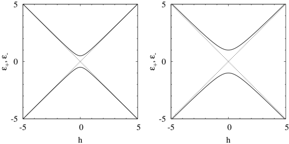
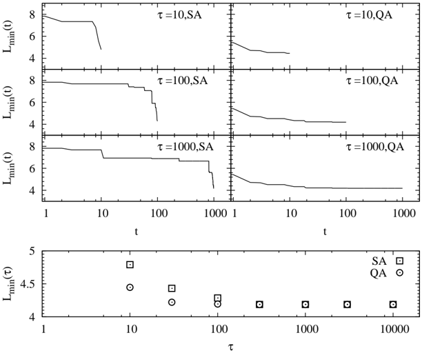
Fig. 2. Eigenenergies of the single spin system under longitudinal and transverse magnetic fields for Γ = 0 . 5 (left panel) and Γ = 1 (right panel). The dotted lines represent eigenenergies for Γ = 0.
<details>
<summary>Image 2 Details</summary>
### Visual Description
\n
## Diagram: Band Structure Plots
### Overview
The image presents two identical band structure plots, likely representing the energy (εx, ε') as a function of a parameter 'h'. Both plots display a characteristic "hourglass" shape, indicative of a Dirac cone or similar band crossing. The plots are visually identical, suggesting they may represent the same system under slightly different conditions or a comparison of two different calculations.
### Components/Axes
Each plot has the following components:
* **X-axis:** Labeled "h", ranging from approximately -5 to 5. The units are not specified.
* **Y-axis:** Labeled "εx, ε'", ranging from approximately -5 to 5. The units are not specified, but likely represent energy.
* **Curves:** Each plot contains two curves, forming an "X" shape that intersects at the origin (h=0, εx, ε'=0). The curves appear to be symmetric with respect to both axes.
* **Plot Arrangement:** Two plots are arranged side-by-side horizontally.
### Detailed Analysis or Content Details
Both plots exhibit the same features. Let's analyze one plot and assume the other is identical.
* **Curve 1 (Upper):** This curve slopes downward from approximately (h=-5, εx, ε' = 5) to (h=0, εx, ε' = 0), then slopes upward to (h=5, εx, ε' = 5). It appears to be a linear relationship in each segment.
* **Curve 2 (Lower):** This curve slopes upward from approximately (h=-5, εx, ε' = -5) to (h=0, εx, ε' = 0), then slopes downward to (h=5, εx, ε' = -5). It also appears to be a linear relationship in each segment.
* **Intersection:** Both curves intersect at the origin (h=0, εx, ε' = 0).
* **Symmetry:** The plots are symmetric about both the x and y axes.
Due to the nature of the plot (lines without data points), precise numerical values cannot be extracted. The values provided are approximate based on visual inspection.
### Key Observations
* The identical nature of the two plots suggests they represent the same underlying physics.
* The "hourglass" shape is a hallmark of Dirac cones or similar band crossings, often found in materials with topological properties.
* The linear segments of the curves suggest a simple dispersion relation in those regions.
### Interpretation
The plots likely represent the electronic band structure of a material. The "hourglass" shape indicates a linear dispersion relation near the crossing point, which is characteristic of massless Dirac fermions. This suggests the material may exhibit interesting electronic properties, such as high mobility and topological protection. The parameter 'h' could represent a momentum component or some other relevant physical quantity. The fact that the two plots are identical suggests that the system is not sensitive to some parameter that might have been varied between the two calculations. The absence of specific labels or a caption makes it difficult to determine the exact material or system being studied. The plots are a visual representation of a mathematical relationship between energy and a parameter, and do not contain specific data points beyond the curves themselves.
</details>
and the initial state is set to be the corresponding eigenstate, the good quantum number is conserved. Then when we perform the quantum annealing method based on the real-time dynamics, we should take care of the symmetries of the considered Hamiltonian. From this, we can obtain the ground state of the considered system in the adiabatic limit if there is no level crossing. In practice, however, since we change magnetic field with finite speed, a nonadiabatic transition is inevitable. To show this fact, we consider a single spin system under longitudinal and transverse magnetic fields. The Hamiltonian of this system is given by
<!-- formula-not-decoded -->
Since the eigenenergies are /epsilon1 ± = ± √ h 2 +Γ 2 , the smallest value of the energy difference between the ground state and the excited state is 2Γ at h = 0 as shown in Fig. 2.
Suppose we consider the single spin system under time-dependent longitudinal magnetic field and fixed transverse magnetic field. The Hamiltonian is given by
<!-- formula-not-decoded -->
where we adopt h ( t ) = vt as time-dependent longitudinal field. Here we set t = -∞ as the initial time. The initial state is set to be the ground
state of the Hamiltonian at the initial time | ψ ( t = -∞ ) 〉 = |↓〉 . The ground state at t = + ∞ in the adiabatic limit is | ψ (ad) ( t = + ∞ ) 〉 = |↑〉 . Then a characteristic value which represents the nature of this dynamics is a probability of staying in the ground state at t = + ∞ which is defined by
∣ ∣ The probability of staying in the ground state should depend on the sweeping speed v and the characteristic energy gap and can be obtained by the Landau-Zener-St¨ uckelberg formula: 90-92
<!-- formula-not-decoded -->
<!-- formula-not-decoded -->
where ∆ E and ∆ m represent the energy gap at the avoided level-crossing point and the difference of the magnetizations in the adiabatic limit, respectively. In this case ∆ E = 2Γ and ∆ m = 2.
In many cases, typical shape of energy structure can be approximated by simple systems such as the single spin system. Then the knowledge of the simple transitions such as the Landau-Zener-St¨ ukelberg transition and the Rosen-Zener transition 93 is useful to analyze the efficiency of the quantum annealing based on the real-time dynamics.
## 3.4. Experiments
Transverse field response of the Ising model has been also established in experimentally. 94-103 A dipolar-coupled disordered magnet LiHo x Y 1 -x F 4 has easy-axis anisotropy and can be represented by the Ising model. 104,105 If we apply the longitudinal magnetic field (in other words, the magnetic field is parallel to the easy-axis), phase transition does not take place. 106,107 However, when we apply the transverse magnetic field (in other words, the magnetic field is perpendicular to the easy-axis), phase transitions occur and interesting dynamical properties shown in Ref.[ 6] were observed. In the phase diagram of this material, there are three phases. The ferromagnetic phase appears at intermediate temperature and low transverse magnetic field, whereas at low temperature and low transverse magnetic field, the glassy critical phase 108 appears. The paramagnetic phase exists at the other region. The glassy critical phase exhibits slow relaxation in general. It found that the characteristic relaxation time obtained by ac field susceptibility for
quantum cooling in which we decrease transverse field after temperature is decreased is lower than that for temperature cooling case. 6 From this result, it has been expected that the effect of the quantum fluctuation helps us to obtain the best solution of the optimization problem.
## 4. Optimization Problems
Optimization problems are defined by composition elements of the considered problem and real-valued cost/gain function. They are problems to obtain the best solution such that the cost/gain function takes the minimum/maximum value. In general, the number of candidate solutions increases exponentially with the number of composition elements in optimization problems. Although we can obtain the best solution by a brute force in principle, it is difficult to obtain the best solution by such a naive method in practice. Then we have to invent an innovative method for obtaining the best solution in a practical time and limited computational resource. Optimization problems can be expressed by the Ising model in many cases. Once optimization problems are mapped onto the Ising model, we can use methods that have been considered in statistical physics and computational physics such as the quantum annealing.
In the anterior half of this section, we explain the correspondence between the Ising model and the traveling salesman problem which is one of famous optimization problems. We demonstrate the quantum annealing based on the quantum Monte Carlo simulation for this problem. In the posterior half, we explain the clustering problem as the example expressed by the Potts model which is a straightforward extension of the Ising model.
## 4.1. Traveling Salesman Problem
In this section, we consider the traveling salesman problem which is one of famous optimization problems. The setup of the traveling salesman problem is as follows:
- There are N cities.
- We move from the i -th city to the j -th city where the distance between them is /lscript i,j .
- We can pass through a city only once.
- We return the initial city after we pass through all the cities.
The traveling salesman problem is to find the minimum path under above conditions. The length of a path is given by
<!-- formula-not-decoded -->
where c a denotes the city where we pass through at the a -th step. In the traveling salesman problem, the length of a path is a cost function. From the fourth condition, the following relation should be satisfied:
<!-- formula-not-decoded -->
In terms of mathematics, the traveling salesman problem is to find { c a } N a =1 so as to minimize the path L under the above four conditions.
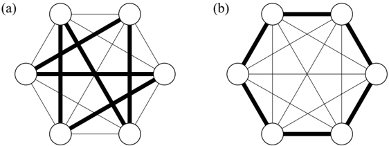
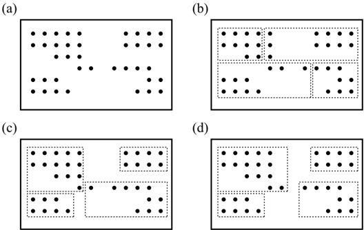
If the number of cities N is small, it is easy to obtain the shortest path by a brute force. We can easily find the best solution of the traveling salesman problem for N = 6 shown in Fig. 3. Figure 3 (a) and (b) represent a bad solution and the best solution where the length of the path L is minimum, respectively. As the number of cities increases, the traveling salesman problem becomes seriously difficult since the number of candidate solutions is ( N -1)! / 2. Then if we want to deal with the traveling salesman problem with large N , we have to adopt smart and easy practical methods such as the simulated annealing instead of a brute force. To use the simulated annealing, we map the traveling salesman problem onto the Ising model with a couple of constraints as follows.
We consider N × N two-dimensional lattice. Let n i,a be the microscopic state which represents the state at the i -th city at the a -th step. The value of n i,a can be taken either 0 or 1. If we pass through the i -th city at the
Fig. 3. Traveling salesman problem for N = 6. Thin lines and thick lines denote the permitted paths and selected paths, respectively. (a) Bad solution. (b) The best solution in which the length of the path is minimum.
<details>
<summary>Image 3 Details</summary>
### Visual Description
\n
## Diagram: Network Topology Comparison
### Overview
The image presents a comparison of two network topologies, labeled (a) and (b). Both diagrams depict nodes connected by edges, representing a network structure. The diagrams are visually similar but differ in the number of nodes and the pattern of connections. There are no axis labels, legends, or numerical data present.
### Components/Axes
The diagrams consist of:
* **Nodes:** Represented by white circles.
* **Edges:** Represented by black lines connecting the nodes.
* **Labels:** "(a)" and "(b)" identify each network topology.
### Detailed Analysis or Content Details
**Diagram (a):**
* Number of Nodes: 6
* The nodes are arranged approximately in a hexagonal shape.
* Edges: There are approximately 9 edges connecting the nodes. The connections are not fully connected, with several nodes having fewer connections than others. The connections appear somewhat random, lacking a clear pattern.
**Diagram (b):**
* Number of Nodes: 6
* The nodes are arranged in a perfect hexagonal shape.
* Edges: There are approximately 12 edges connecting the nodes. All nodes are connected to every other node, forming a complete graph. The outer perimeter of the hexagon is formed by a continuous set of edges.
### Key Observations
* Diagram (a) represents a sparse network with fewer connections, while diagram (b) represents a dense, fully connected network.
* The arrangement of nodes in diagram (b) is more regular and symmetrical than in diagram (a).
* Both diagrams have the same number of nodes.
### Interpretation
The diagrams likely illustrate the difference between two types of network topologies. Diagram (a) could represent a network with limited redundancy or a network that is still under development. Diagram (b) represents a highly robust network where any node failure does not disrupt connectivity between other nodes. The comparison highlights the trade-offs between cost (number of connections) and reliability (network resilience). The diagrams are abstract representations and do not provide specific information about the nature of the nodes or the purpose of the network. They serve as a visual aid to understand the concept of network topology and its impact on network characteristics.
</details>
a -th step, n i,a is unity whereas n i,a = 0 if we do not pass through the i -th city at the a -th step. The third condition can be represented by
<!-- formula-not-decoded -->
Furthermore, since it is obvious that we can pass through only one city at the a -th step, this constraint is expressed by
<!-- formula-not-decoded -->
Then the length of the path L can be rewritten as
<!-- formula-not-decoded -->
where the Ising spin variable σ z i,a = ± 1 is defined by
<!-- formula-not-decoded -->
Here we used the following relation derived by Eqs. (84) and (85):
<!-- formula-not-decoded -->
Then the length of the path can be represented by the Ising spin Hamiltonian on N × N two-dimensional lattice. In general, it is difficult to obtain the stable state of the Ising model with some constraints regarded as some kind of frustration which will be shown in Sec. 5.2.
## 4.1.1. Monte Carlo Method
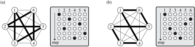
We explain how to implement the Monte Carlo method in the traveling salesman problem. We cannot use the single-spin-flip method which was explained in Sec. 3.1 because of existence of two constraints given by Eqs. (84) and (85). The simplest way of transition between states is realized by flipping four spins simultaneously as shown in Fig. 4.
Suppose we consider the case that we pass through at the i -th city at the a -th step and pass through at the j -th city at the a ′ -th step, which is described as
<!-- formula-not-decoded -->
Fig. 4. The simplest way of flipping method in traveling salesman problem. Transition between the state depicted in (a) and that depicted in (b) occurs. In this case, i = 3, j = 6, a = 2, and a ′ = 5.
<details>
<summary>Image 4 Details</summary>
### Visual Description
\n
## Diagram: Network Evolution with Step Progression
### Overview
The image presents two diagrams, labeled (a) and (b), illustrating the evolution of a network over a series of steps. Each diagram consists of a network graph alongside a grid representing the state of the network at each step. The network graphs have six nodes, numbered 1 through 6, and the grids are 6x6, with each cell representing a possible state. The diagrams demonstrate how connections within the network change over time, as indicated by the filled cells in the grid.
### Components/Axes
Each diagram contains two main components:
1. **Network Graph:** A graph with six nodes (1-6) connected by lines representing edges.
2. **Step Progression Grid:** A 6x6 grid labeled with numbers 1-6 along the top, and an arrow labeled "step" indicating the progression of time. The grid cells are filled with black circles to indicate the state of the network at each step.
### Detailed Analysis or Content Details
**Diagram (a):**
* **Network Graph:** The network graph shows connections between nodes 1-2, 1-3, 1-5, 2-3, 2-4, 3-4, 3-5, 4-5, 5-6, and 6-1.
* **Step Progression Grid:**
* Step 1: Cells (1,1), (2,2), (3,3), (4,4), (5,5), (6,6) are filled.
* Step 2: Cells (1,2), (2,3), (3,4), (4,5), (5,6), (6,1) are filled.
* Step 3: Cells (1,3), (2,4), (3,5), (4,6), (5,1), (6,2) are filled.
* Step 4: Cells (1,4), (2,5), (3,6), (4,1), (5,2), (6,3) are filled.
* Step 5: Cells (1,5), (2,6), (3,1), (4,2), (5,3), (6,4) are filled.
* Step 6: Cells (1,6), (2,1), (3,2), (4,3), (5,4), (6,5) are filled.
**Diagram (b):**
* **Network Graph:** The network graph shows connections between nodes 1-2, 2-3, 3-4, 4-5, 5-6, 6-1, 1-6, and 2-5.
* **Step Progression Grid:**
* Step 1: Cells (1,1), (2,2), (3,3), (4,4), (5,5), (6,6) are filled.
* Step 2: Cells (1,2), (2,3), (3,4), (4,5), (5,6), (6,1) are filled.
* Step 3: Cells (1,3), (2,4), (3,5), (4,6), (5,1), (6,2) are filled.
* Step 4: Cells (1,4), (2,5), (3,6), (4,1), (5,2), (6,3) are filled.
* Step 5: Cells (1,5), (2,6), (3,1), (4,2), (5,3), (6,4) are filled.
* Step 6: Cells (1,6), (2,1), (3,2), (4,3), (5,4), (6,5) are filled.
### Key Observations
Both diagrams show a cyclical pattern in the step progression grid, where the filled cells shift diagonally across the grid with each step. The network graphs differ in their connections, indicating different network structures. Diagram (a) has a more interconnected network, while diagram (b) has a more structured, ring-like network.
### Interpretation
These diagrams likely represent a simulation or model of network dynamics. The step progression grid illustrates how the state of the network evolves over time, while the network graph shows the underlying connections between nodes. The differences between diagrams (a) and (b) suggest that the initial network structure influences the evolution of the network. The cyclical pattern in the grid indicates a periodic behavior or a repeating process within the network. This could be a model of information propagation, resource allocation, or other network-based phenomena. The diagrams demonstrate how the topology of a network can affect its dynamic behavior. The filled cells in the grid could represent activated nodes or connections, and the shifting pattern could represent the spread of activity through the network.
</details>
The trial state generated by flipping four spins is as follows:
<!-- formula-not-decoded -->
The heat-bath method and the Metropolis method can be adopted for the transition probability between the present state and the trial state. In Fig. 4, i = 3, j = 6, a = 2, and a ′ = 5.
It should be noted that without loss of generality the initial condition can be set as
<!-- formula-not-decoded -->
/negationslash and thus we can fix the states at the first step ( a = 1) during calculation. The number of interactions in which we try to flip all spins in each Monte Carlo step is ( N -1)( N -2) / 2.
## 4.1.2. Quantum Annealing
In order to perform the quantum annealing, we introduce the transverse field as the quantum fluctuation effect as shown in Sec. 3. The quantum Hamiltonian is given by
<!-- formula-not-decoded -->
where the first-term corresponds to the length of path and the second-term denotes the transverse field. We can map this quantum Hamiltonian on N × N two-dimensional lattice onto N × N × m three-dimensional Ising model as well as the case which was considered in Sec. 3.1. The effective classical
Hamiltonian derived by the Suzuki-Trotter decomposition is written as
<!-- formula-not-decoded -->
In the quantum annealing procedure, we have to take care of the constraints given by Eqs. (84) and (85) as stated before. Then the simplest way of changing state is to flip simultaneously four spins on the same layer ( m is fixed) along the Trotter axis.
## 4.1.3. Comparison with Simulated Annealing and Quantum Annealing
In order to demonstrate the comparison with the simulated annealing and the quantum annealing, we perform the Monte Carlo simulation for the traveling salesman problem. As an example, we consider N = 20 cities depicted in Fig. 5 (a). The positions of these cities were generated by pair of uniform random numbers (0 ≤ x i , y i ≤ 1). The time schedules of temperature T ( t ) for the simulated annealing and transverse field Γ( t ) for the
Fig. 5. Traveling salesman problem for N = 20. (a) Positions of cities. (b) The best solution in which the length of the path is minimum.
<details>
<summary>Image 5 Details</summary>
### Visual Description
\n
## Scatter Plots: Two-Panel Comparison
### Overview
The image presents two scatter plots, labeled (a) and (b), both depicting a relationship between two variables, 'x' and 'y'. Plot (a) shows a random distribution of points, while plot (b) displays a connected line graph derived from a set of points. Both plots share the same x and y axis scales.
### Components/Axes
Both plots share the following:
* **X-axis:** Labeled "x", ranging from 0.0 to 1.0 with tick marks at 0.1 intervals.
* **Y-axis:** Labeled "y", ranging from 0.0 to 1.0 with tick marks at 0.1 intervals.
* **Plot (a):** Contains approximately 20 circular data points scattered across the plot area.
* **Plot (b):** Contains approximately 10 circular data points connected by straight lines, forming a polygonal path.
### Detailed Analysis or Content Details
**Plot (a):**
The points in plot (a) appear randomly distributed. Approximate coordinates (with uncertainty of ±0.02) are:
* (0.02, 0.02)
* (0.05, 0.62)
* (0.08, 0.85)
* (0.12, 0.55)
* (0.15, 0.42)
* (0.20, 0.35)
* (0.25, 0.68)
* (0.30, 0.48)
* (0.35, 0.32)
* (0.40, 0.50)
* (0.45, 0.40)
* (0.50, 0.25)
* (0.55, 0.60)
* (0.60, 0.52)
* (0.65, 0.22)
* (0.70, 0.45)
* (0.75, 0.65)
* (0.80, 0.58)
* (0.85, 0.42)
* (0.90, 0.38)
**Plot (b):**
The line in plot (b) exhibits a non-monotonic trend. Approximate coordinates (with uncertainty of ±0.02) are:
* (0.00, 0.00)
* (0.10, 0.95)
* (0.20, 0.70)
* (0.30, 0.35)
* (0.40, 0.40)
* (0.50, 0.55)
* (0.60, 0.62)
* (0.70, 0.48)
* (0.80, 0.20)
* (0.90, 0.40)
### Key Observations
* Plot (a) shows no clear correlation between x and y.
* Plot (b) demonstrates a complex relationship between x and y, with increasing and decreasing segments. The line initially rises sharply, then declines, fluctuates, and ends with a slight increase.
### Interpretation
The two plots likely represent different aspects of the same underlying phenomenon or two distinct phenomena. Plot (a) could represent a random sample or a system with no apparent linear relationship between the variables. Plot (b) suggests a more deterministic or process-driven relationship, where the value of 'y' is influenced by 'x' in a non-linear manner. The shape of the curve in plot (b) could indicate a cyclical process, a response to a series of inputs, or a complex interaction between multiple factors. Without further context, it's difficult to determine the specific meaning of these plots, but they clearly demonstrate contrasting data patterns. The use of a connected line in (b) implies that the data points are ordered and represent a sequence or a trajectory.
</details>
quantum annealing are defined as
<!-- formula-not-decoded -->
where T 0 and Γ 0 are temperature and transverse field at the final time ( t = τ ), and T 0 + T 1 and Γ 0 +Γ 1 are temperature and transverse field at the initial time ( t = 0). The value of τ -1 indicates the annealing speed, and the annealing speed becomes slow as the value of τ increases. In our simulations, we adopt T 0 = Γ 0 = 0 . 01 and T 1 = Γ 1 = 5. Furthermore, we fix the transverse field as Γ = 0 during the simulation in the simulated annealing and the temperature as T = 0 . 01 during the simulation in the quantum annealing.
<!-- formula-not-decoded -->
We execute 100 independent simulations of simulated annealing based on the heat-bath type Monte Carlo method where each initial state generated by the uniform random number is different. To compare the efficiency of the simulated annealing and quantum annealing in an equitable manner, in the quantum annealing, the Trotter number is putted as m = 10, and we execute 10 independent simulations. We also calculate the minimum length of path L min ( t ) := min { L ( t ′ ) | 0 ≤ t ′ ≤ t } . It should be noted that L min ( t ) is a monotonic decreasing function. The upper panel of Fig. 6 shows the time dependence of minimum length of path L min ( t ) for various τ . From the upper panel of Fig. 6, we can see that the convergence of minimum length of path in the quantum annealing is faster than that in the simulated annealing. We also show the sweeping time τ dependence of the minimum length of path at the final state L min ( τ ) in the lower panel of Fig. 6. This figure indicates that the obtained solution in the quantum annealing is always better than that in the simulated annealing. Figure 5 (b) shows the obtained best solution in both the simulated annealing and the quantum annealing with slow schedule.
In this way, we can obtain a better solution (in this case, the best solution) by both annealing methods with slow schedule. Moreover, in our calculation, the convergence of solution in the quantum annealing is faster than that in the simulated annealing, and the obtained solution in the quantum annealing is better than that in the simulated annealing regardless of sweeping time τ . Thus, we can say that the quantum annealing method is appropriate as the annealing method for the traveling salesman problem in comparison with the simulated annealing. This fact has been confirmed in some researches. 86,109
Fig. 6. (Upper panel) Time dependence of minimum length of path L min ( t ) for τ = 10, 100, and 1000 obtained by the simulated annealing (SA) and the quantum annealing (QA). (Lower panel) Sweeping-time τ dependence of minimum length of path at the final state L min ( τ ) obtained by the simulated annealing indicated by squares and the quantum annealing indicated by circles.
<details>
<summary>Image 6 Details</summary>
### Visual Description
## Chart: Minimum Length vs. Time and Tau
### Overview
The image presents a series of line graphs and a scatter plot examining the relationship between minimum length (Lmin(t)) and time (t), as well as Lmin(T) and tau (τ). The data is presented for two different methods, labeled "SA" (Simulated Annealing) and "QA" (Quasi-Newton Algorithm). The graphs explore how Lmin(t) changes over time for different values of τ, and how Lmin(T) varies with τ.
### Components/Axes
* **Top Section:** Contains six line graphs arranged in a 3x2 grid.
* **Y-axis (all graphs):** Lmin(t) - labeled "Lmin(t)", ranging from approximately 4 to 8.
* **X-axis (all graphs):** t - labeled "t", on a logarithmic scale from 1 to 1000.
* **Titles (each graph):** Indicate the value of τ and the method used (e.g., "τ=10,SA").
* **Bottom Section:** A scatter plot.
* **Y-axis:** Lmin(T) - labeled "Lmin(T)", ranging from approximately 4 to 5.5.
* **X-axis:** τ - labeled "τ", on a logarithmic scale from 1 to 10000.
* **Legend (top-right):**
* SA (Simulated Annealing) - represented by a black square.
* QA (Quasi-Newton Algorithm) - represented by a white circle.
### Detailed Analysis or Content Details
**Top Section - Line Graphs:**
* **τ=10, SA (Top-Left):** The line starts at approximately 7.8 and rapidly decreases to around 5.5 by t=10. It then plateaus around 5.5 until t=100, after which it decreases slightly to approximately 5.2 by t=1000.
* **τ=10, QA (Top-Right):** The line starts at approximately 7.5 and gradually decreases to around 5.5 by t=1000. The decrease is relatively smooth and consistent.
* **τ=100, SA (Middle-Left):** The line starts at approximately 7.8 and decreases in steps to around 5.2 by t=100. It remains relatively constant until t=1000, where it decreases slightly to approximately 5.0.
* **τ=100, QA (Middle-Right):** The line starts at approximately 7.5 and gradually decreases to around 5.5 by t=1000. The decrease is smoother than the SA method.
* **τ=1000, SA (Bottom-Left):** The line starts at approximately 7.8 and decreases rapidly in steps to around 5.2 by t=100. It remains relatively constant until t=1000, where it decreases slightly to approximately 5.0.
* **τ=1000, QA (Bottom-Right):** The line starts at approximately 7.5 and decreases gradually to around 5.5 by t=1000. The decrease is smoother than the SA method.
**Bottom Section - Scatter Plot:**
* **SA (Black Squares):**
* τ=10: Lmin(T) ≈ 5.3
* τ=100: Lmin(T) ≈ 5.1
* τ=1000: Lmin(T) ≈ 4.9
* τ=10000: Lmin(T) ≈ 4.8
* **QA (White Circles):**
* τ=10: Lmin(T) ≈ 5.1
* τ=100: Lmin(T) ≈ 5.0
* τ=1000: Lmin(T) ≈ 4.9
* τ=10000: Lmin(T) ≈ 4.8
### Key Observations
* For all values of τ, the SA method exhibits a more stepwise decrease in Lmin(t) compared to the smoother decrease observed with the QA method.
* As τ increases, the initial value of Lmin(t) remains relatively constant around 7.8-7.5.
* The final value of Lmin(t) at t=1000 appears to converge towards approximately 5.0-5.5 for both methods and all values of τ.
* The scatter plot shows that Lmin(T) decreases slightly as τ increases for both SA and QA methods. The decrease is more pronounced for the SA method.
* The QA method consistently yields slightly lower values of Lmin(T) compared to the SA method for all values of τ.
### Interpretation
The data suggests that the minimum length (Lmin) decreases over time (t) for both Simulated Annealing (SA) and Quasi-Newton Algorithm (QA) methods. The rate of decrease is influenced by the parameter τ. Larger values of τ seem to lead to a more gradual decrease in Lmin(t) for both methods. The scatter plot indicates that the final minimum length (Lmin(T)) is also affected by τ, with larger τ values resulting in slightly lower Lmin(T).
The difference in the behavior of the two methods (SA vs. QA) is notable. SA exhibits a more discrete, stepwise decrease, likely due to its stochastic nature, while QA demonstrates a smoother, more continuous decrease, characteristic of gradient-based optimization methods. The QA method consistently achieves slightly lower final minimum lengths, suggesting it might be more efficient in finding optimal solutions in this context.
The logarithmic scale on the x-axis (t and τ) indicates that the effects of time and τ are likely non-linear. The initial rapid decrease in Lmin(t) followed by a plateau suggests that the system quickly reaches a state of diminishing returns, where further optimization yields smaller improvements. The convergence of Lmin(t) towards a similar value for all τ values at t=1000 suggests that the system is approaching a stable state, regardless of the initial value of τ.
</details>
## 4.2. Clustering Problem
In Sec. 4.1, we explained the traveling salesman problem which can be mapped onto the Ising model with some constraints. Many optimization problems can also be mapped onto the Ising model. However, there are a number of optimization problems that can be described by the other models which are straightforward extensions of the Ising model. In this section, we review the concept of clustering problem as such an example.
Clustering problem is also one of important optimization problems in information science and engineering. 12-14 We need to categorize much data in the real world according to its contents in various situations. For instance, suppose we play stock market. In order to see the socioeconomic situation, we want to extract efficiently important information related to
stock market from an enormous quantity of information in news sites and newspapers. In this case, it is better to categorize many articles in news sites and newspapers according to their contents. This is an example of clustering problem which is adopted for many applications in wide area of science such as cognitive science, social science, and psychology. The clustering problem is to divide the whole set into a couple of subsets. Here we refer to the subsets as 'cluster'.
Figure 7 shows schematic picture of the clustering problem. Suppose we consider much data in the whole set which represents the square frame in Fig. 7 (a). The points in Fig. 7 denote individual data. In the clustering problem, our target is to find which the best division is. Figure 7 (b), (c), and (d) represent typical clustering states Σ 1 , Σ 2 , and Σ ∗ , respectively. The states Σ 1 and Σ 2 are an unstable solution and a metastable solution, respectively. The state Σ ∗ denotes the best solution of clustering problem.
In order to consider how to implement the quantum annealing, the clustering problem can be described by the Potts model with random interac-
Fig. 7. Schematic pictures of clustering problem. The points represent data and the square denote the whole set. (a) Data set. (b) Unstable solution Σ 1 . (c) Metastable solution Σ 2 . (d) The best solution Σ ∗ .
<details>
<summary>Image 7 Details</summary>
### Visual Description
\n
## Diagram: Dot Distribution Patterns
### Overview
The image presents four distinct arrangements of dots within rectangular frames, labeled (a) through (d). Each frame contains a collection of black dots, and some frames also include dotted-line rectangles partitioning the space. The purpose appears to be illustrating different spatial distributions or groupings of points. There are no axes, legends, or numerical values provided.
### Components/Axes
The image consists of four rectangular frames, each labeled with a letter: (a), (b), (c), and (d). Each frame contains a varying number of black dots. Frames (b), (c), and (d) also contain dotted-line rectangles that divide the space into smaller regions. There are no axis labels or legends.
### Detailed Analysis or Content Details
* **Frame (a):** Approximately 30-35 dots are scattered across the frame. The dots are not organized into distinct clusters, but appear relatively evenly distributed, with a slightly higher density in the top-left corner.
* **Frame (b):** Approximately 25-30 dots are present. The frame is divided into four regions by dotted lines. The top-right region contains approximately 8-10 dots. The top-left region contains approximately 4-6 dots. The bottom-left region contains approximately 6-8 dots. The bottom-right region contains approximately 6-8 dots.
* **Frame (c):** Approximately 30-35 dots are present. The frame is divided into three regions by dotted lines. The top-left region contains approximately 10-12 dots. The top-right region contains approximately 6-8 dots. The bottom region contains approximately 12-14 dots.
* **Frame (d):** Approximately 25-30 dots are present. The frame is divided into three regions by dotted lines. The top-left region contains approximately 8-10 dots. The top-right region contains approximately 6-8 dots. The bottom region contains approximately 10-12 dots.
### Key Observations
The primary difference between the frames lies in the organization of the dots. Frame (a) shows a random or uniform distribution, while frames (b), (c), and (d) demonstrate a partitioned distribution, where dots are grouped within defined regions. The number of dots in each region varies across frames (b), (c), and (d).
### Interpretation
The image likely illustrates different spatial patterns or distributions of data points. Frame (a) could represent a control condition or a baseline distribution. Frames (b), (c), and (d) could represent different experimental conditions where the points are constrained or grouped into specific areas. The dotted lines suggest boundaries or categories. The varying number of dots within each region in frames (b), (c), and (d) could indicate different levels of concentration or preference for those regions. Without further context, it's difficult to determine the specific meaning of these patterns, but they could represent anything from population density to experimental results. The image is a visual representation of spatial data, but lacks quantitative data to support a more detailed analysis.
</details>
tions d . The Hamiltonian of the Potts model is given by
<!-- formula-not-decoded -->
where the summation runs over all pairs of the i -th and j -th data. The spin variable σ i represents individual data. Here the value of Q represents the number of clusters. When σ i = σ j , the i -th and j -th data are in the same cluster. It is natural to adopt ferromagnetic/antiferromagnetic interaction between data in the same/different cluster. It should be noted that the Potts model is a straightforward extension of the Ising model since the Potts model is equivalent to the Ising model if Q = 2. Then the clustering problem is a problem to obtain the ground state of the Hamiltonian of the Potts model with given random interactions. Here we assume that the number of clusters is fixed.
Next we explain how to introduce quantum field in order to perform the quantum annealing. In optimization problems which can be represented by the Ising model, we can use transverse field as the quantum fluctuation which is represented as -Γ ∑ i σ x i . However, we cannot use this transverse field -Γ ∑ i σ x i for the clustering problem directly, since the matrix which represents the state is Q × Q matrix. Thus, we generalize the x -component of the Pauli matrix of the Ising model as follows:
<!-- formula-not-decoded -->
where E Q and I Q represent the Q × Q unit matrix and the Q × Q matrix whose all elements are unity. By using this generalized Pauli matrix, we can apply the quantum annealing for clustering problem. 12-14 Here we consider the following Hamiltonian:
<!-- formula-not-decoded -->
d In practice, we do not know { J ij } and have to estimate interactions when we consider the clustering problem. However, we assume the Hamiltonian for simple explanation. As shown in this section, the implementation method does not depend on the specific form of interactions.
where N is the number of individual data. As well as the case for the Ising model, we can calculate the partition function of the Hamiltonian:
<!-- formula-not-decoded -->
∣ ∣ ∣ ∣ where | Σ k 〉 represents the direct-product space of N spins:
$$\sum _ { k = 1 } ^ { \infty } ( o _ { 1 , k } ) \otimes ( o _ { 2 , k } ) \otimes \cdots$$
There are two elements 〈 Σ k | e -β ˆ H Potts /m | Σ ′ k 〉 and 〈 Σ ′ k | e -β ˆ H (Potts) q /m | Σ k +1 〉 . These factors are calculated as follows:
$$( \sum _ { j } e ^ { - \beta H_P ( t s , m ) } | z _ { k } | ^ { 2 } ) = \exp ( \frac { \sum _ { i = 1 } ^ { N } z _ { i } } { m } \sum _ { i = 1 } ^ { N } \left[ e ^ { - \beta H_P ( t s , m ) } + \frac { 1 } { e ^ { - \beta H_P ( t s , m ) } ( 1 - q ) } \right] .$$
$$\sum _ { m = 1 } ^ { N } \sum _ { k = 1 } ^ { m } [ e ^ { - g x ( Potts ) / m } \sum _ { i = 1 } ^ { k } \left | e ^ { - g x ( - q ) - 1 } \right | ] .$$
By using the above expressions, we can perform the quantum Monte Carlo simulation as well as the Ising model with transverse field. If the spin variable is not S = 1 / 2 Ising spin as in the case just described, we can implement the quantum annealing by considering appropriate quantum field. There are some studies that the quantum annealing succeeds to obtain the better solution than the simulated annealing for clustering problems. 12-14
## 5. Relationship between Quantum Annealing and Statistical Physics
In the preceding sections we explained the Ising model, a couple of implementation methods of the quantum annealing, and the optimization problems. There are a couple of studies that clarify the efficiency and feature of the quantum annealing in terms of statistical physics. In this section we take two examples which display relationship between quantum annealing and statistical physics focusing on the thermal fluctuation effect and the quantum fluctuation effect for ordering phenomena. In the first half, we
review the Kibble-Zurek mechanism which characterizes the efficiency of the quantum annealing for systems where a second-order phase transition occurs comparing with the efficiency of the simulated annealing. In the last half, we show similarities and differences between thermal fluctuation and quantum fluctuation for frustrated Ising spin systems.
## 5.1. Kibble-Zurek Mechanism
In statistical physics, it has been an important topic to investigate the ordering process in systems where a phase transition takes place. 110-116 Especially, dynamical properties during changing control variables such as temperature and external fields are interesting. 111,113,115 Recently, the Kibble-Zurek mechanism has been drawing attention not only in statistical physics and condensed matter physics but also for the quantum annealing. In this section, we explain the Kibble-Zurek mechanism relating to a dynamics which passes across a second-order phase transition point. The Kibble-Zurek mechanism can make clear what happens in systems where the second-order phase transition occurs during the simulated annealing and the quantum annealing from a viewpoint of statistical physics. Before we consider the efficiency of the quantum annealing comparing with the simulated annealing by using the Kibble-Zurek mechanism, we show the general feature of the Kibble-Zurek mechanism.
As an example, we consider the Kibble-Zurek mechanism in the ferromagnetic system where the second-order phase transition occurs at finite temperature. At the second-order phase transition point, the correlation length diverges in the equilibrium state, and thus the relaxation time should be infinite. Hence, the system cannot reach the equilibrium state, when we decrease temperature to the transition temperature with finite speed. Furthermore, since the relaxation time is long around the transition temperature, it is difficult to equilibrate the system. Here, we assume that growth of correlation length stops at the temperature where the system is less able to reach the equilibrium state. If we decrease temperature slow enough, the system can reach the equilibrium state even near the transition point. Thus, it is expected that the value of stopped correlation length because of the long relaxation time depends on the annealing speed. As we will see below, the value of stopped correlation length can be scaled by the annealing speed.
To consider the second-order phase transition at finite temperature in
the ferromagnetic systems, we define the dimensionless temperature g as
$$g = \frac { T - T _ { c } } { T _ { c } } ,$$
where T c is the phase transition temperature. When the absolute value of g is small, it is believed that the scaling ansatz is valid. By the scaling ansatz, the temperature-dependent correlation length ξ ( g ) is given as 117
$$\{ g \} \times \{ g \} ^ { - 1 } ,$$
where ν is one of the critical exponents. Moreover, the relaxation time τ rel is scaled by the following relation: 117
$$T _ { rel } ( g ) \times [ \{ ( g ) \} ^ { 2 } \times | g | ^ { - 2 v }$$
where z is the dynamical critical exponent. Here, we decrease the temperature T ( t ) against the time t as following schedule:
$$\rho ( t ) = \rho _ { c } ( 1 - \frac { t } { T Q } )$$
The value of τ -1 Q corresponds to the annealing speed. When the value of τ Q is large/small, the system is annealed to low temperature slowly/quickly. At t = 0, the temperature is the phase transition temperature ( T (0) = T c ), and the temperature is zero ( T ( τ Q ) = 0) at t = τ Q . From Eq. (106), the dimensionless temperature g becomes the time-dependent function as follows:
$$g ( t ) = \frac { T ( t ) - T _ { c } } { T _ { c } } = - \frac { t } { T Q }$$
In the Kibble-Zurek mechanism, we assume the following situation:
$$\left\{ \begin{array}{ll} t _ { rel } ( g ( t ) ) < | t | : system can reach equilibrium state \\ t _ { rel } ( g ( t ) ) > | t | : system cannot reach equilibrium state \end{array} \right.$$
where | t | is a remaining time to transition temperature. That is, when a remaining time | t | is longer/shorter than the relaxation time τ rel ( g ( t )), the system can/cannot reach the equilibrium state. Note that the value of considered t should be negative since the relaxation time diverges before the temperature reaches the transition temperature ( t = 0). From this assumption, the time ˜ t at which the system is less able to reach the equilibrium state is defined by following relation:
$$\tau _ { rel } ( g ( t ) ) = [ t ].$$
Furthermore, since we have assumed that the growth of correlation length stops at t = ˜ t , the value of correlation length is always ξ ( g ( ˜ t )) below T ( ˜ t ) as shown in Fig. 8. Moreover, the dimensionless temperature at ˜ t is expressed as
$$g ( t ) = \frac { | t | } { r _ { Q } } = \frac { T _ { re } ( g ( t ) ) } { r _ { Q } }$$
From this relation, g ( ˜ t ) is scaled by the annealing speed, and from Eqs. (104) and (110), the correlation length at t = ˜ t is scaled as follows:
$$g ( t ) x ^ { - \frac { 1 } { Q } } , g ( g ( t ) )$$
Furthermore, the density of domain wall n ( t ) is written as
$$( 1 1 2 )$$
where d is the spatial dimension, and n ( ˜ t ) at t = ˜ t is scaled as follows:
$$n ( t ) \times T _ { Q } ^ { - \frac { d v } { dt } + z v } .$$
For instance, in the ferromagnetic Ising model on two-dimensional lattice ( d = 2, ν = 1) when we adopt the Monte Carlo dynamics based on the single-spin-flip method ( z = 2 . 132), 118 the correlation length and the density of domain wall at t = ˜ t are naively obtained as
$$\frac { - 0 . 3 1 9 } { 7 Q ^ { \circ } } , n ( i ) \approx$$
In this way, in the dynamics which passes across the second-order phase transition point at finite temperature, the correlation length and the density of domain wall (topological defect) are scaled by the annealing speed.
Fig. 8. Schematic of the annealing speed dependence of correlation length ξ ( g ( t )). τ -1 Q is annealing speed and τ Q 1 > τ Q 2 > τ Q 3 . We define ˜ T i := T c (1 + | ˜ t | /τ Q i ) and ˜ ξ i := ξ ( | ˜ t | /τ Q i ). The dotted curve represents correlation length in the equilibrium state.
<details>
<summary>Image 8 Details</summary>
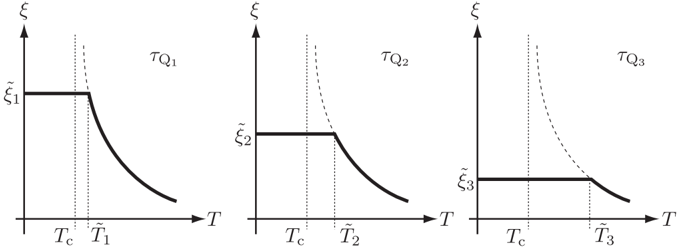
### Visual Description
\n
## Diagram: Strain-Time Curves for Different Quench Rates
### Overview
The image presents three separate graphs illustrating the relationship between strain (ξ) and time (T) during quenching processes. Each graph represents a different quench rate, labeled TQ1, TQ2, and TQ3. The graphs depict the strain evolution as a function of time, with key points marked to indicate critical temperatures and strain levels.
### Components/Axes
* **Y-axis:** Strain (ξ). The scale is not explicitly labeled with numerical values, but it is clear that the strain increases upwards.
* **X-axis:** Time (T). The scale is not explicitly labeled with numerical values.
* **Graphs:** Three separate curves, each representing a different quench rate.
* **Labels:**
* TQ1, TQ2, TQ3: Labels indicating the quench rate for each graph.
* Tc: Critical temperature, marked as a vertical dashed line in each graph.
* T1, T2, T3: Time points after the critical temperature, marked as vertical dashed lines.
* ξ1, ξ2, ξ3: Strain levels at the beginning of the curves.
### Detailed Analysis
**Graph 1 (TQ1):**
* The curve starts at a constant strain level ξ1.
* At time Tc, the strain remains constant for a short duration.
* After time Tc, the strain decreases rapidly and non-linearly until time T1.
* The trend is a steep downward slope.
* Approximate values: ξ1 ≈ 1.0 (relative to the scale), Tc ≈ 0.3 (relative to the scale), T1 ≈ 0.7 (relative to the scale).
**Graph 2 (TQ2):**
* The curve starts at a constant strain level ξ2.
* At time Tc, the strain remains constant for a longer duration than in Graph 1.
* After time Tc, the strain decreases gradually and non-linearly until time T2.
* The trend is a gentler downward slope compared to Graph 1.
* Approximate values: ξ2 ≈ 0.7 (relative to the scale), Tc ≈ 0.4 (relative to the scale), T2 ≈ 0.8 (relative to the scale).
**Graph 3 (TQ3):**
* The curve starts at a constant strain level ξ3.
* At time Tc, the strain remains constant for an even longer duration than in Graph 2.
* After time Tc, the strain decreases slowly and non-linearly until time T3.
* The trend is the gentlest downward slope among the three graphs.
* Approximate values: ξ3 ≈ 0.5 (relative to the scale), Tc ≈ 0.5 (relative to the scale), T3 ≈ 0.9 (relative to the scale).
### Key Observations
* The initial strain levels (ξ1, ξ2, ξ3) decrease as the quench rate increases (TQ1 to TQ3).
* The duration of constant strain at Tc increases as the quench rate increases.
* The rate of strain decrease after Tc decreases as the quench rate increases.
* The graphs demonstrate a clear correlation between quench rate and the resulting strain-time behavior.
### Interpretation
The diagrams illustrate the effect of different quench rates on the strain evolution during a quenching process. A faster quench rate (TQ1) results in a higher initial strain, a shorter period of constant strain at the critical temperature, and a rapid decrease in strain. Conversely, a slower quench rate (TQ3) leads to a lower initial strain, a longer period of constant strain, and a gradual decrease in strain.
The critical temperature (Tc) represents a point where the material's phase transformation begins. The time points (T1, T2, T3) indicate the completion of the transformation process for each quench rate. The differences in strain behavior suggest that the quench rate influences the microstructure and mechanical properties of the material. Faster quenching tends to produce harder, more brittle materials, while slower quenching results in softer, more ductile materials.
The diagrams are a visual representation of the time-temperature-transformation (TTT) curves, commonly used in materials science to understand phase transformations during heat treatment. The curves demonstrate how the cooling rate affects the resulting microstructure and properties of the material.
</details>
This argument is called the Kibble-Zurek mechanism. Since the KibbleZurek mechanism explains the creation of topological defects induced by cooling of the system which takes place the second-order phase transition, this relates to the evolution of cosmic strings by spontaneous symmetry breaking in the Big Bang theory. 119-121 The Kibble-Zurek mechanism can also describe the creation of topological defects in magnetic models, 122,123 superfluid helium systems, 124,125 and Bose-Einstein condensations. 126,127 Next we consider the efficiency of the simulated annealing and the quantum annealing using the Kibble-Zurek mechanism by taking examples which can be treated analytically.
## 5.1.1. Efficiency of Simulated Annealing and Quantum Annealing
Next, we consider the efficiency of the simulated annealing and the quantum annealing according to the Kibble-Zurek mechanism. As an example, we treat the case where the non-domain wall state is the best solution. In this case, the value of n ( ˜ t ) approximately represents the difference between the obtained solution and the best solution. Thus, by using the Kibble-Zurek mechanism, we can compare the efficiency of annealing methods from the behavior of n ( ˜ t ) against the annealing speed. Suppose we solve optimization problems by using annealing methods, we would like to obtain a better solution as fast as possible, in other words, as small τ Q as possible. Then, the comparison obtained by the Kibble-Zurek mechanism is expected to become an useful information for the optimization problems.
As an example, we consider the efficiency of the simulated annealing and the quantum annealing for the random ferromagnetic Ising chain in terms of the Kibble-Zurek mechanism according to Refs. [128,129].
## 5.1.2. Simulated Annealing for Random Ferromagnetic Ising Chain
The model Hamiltonian of the random ferromagnetic Ising chain is given as
$$H = - \sum _ { i } j _ { 0 } ^ { z } o _ { i + 1 } , o _ { i }$$
where J i is the interaction between the i -th site and the ( i +1)-th site. The value of J i is given by the uniform distribution between 0 < J i ≤ 1. The distribution function P (u) ( J i ) is given by
$$p ^ { ( w ) } ( j _ { 1 } ) = \begin{cases} 1 & \text{for } 0 < J_ { 1 } < 1 \\ 0 & \text{otherwise} \end{cases}$$
Since the interaction J i is always positive value, the ground state spin configuration is the all-up spin state or the all-down spin state. In this model, the ferromagnetic transition occurs at zero temperature.
The correlation function between two sites where the distance is r is written as
$$\vert \sigma _ { i } \sigma _ { i + 1 } \vert _ { av } = ( \frac { 1 } { B } \ln \cos h ^ { r } ) ^ { r } , \ldots ( 1 1 7 )$$
where 〈· · · 〉 and [ · · · ] av denote the thermal average and the random average. Physical quantities should depend on the specific spatial pattern of the random interactions { J i } . Then, these averages are defined by
$$( 0 ( J _ { 3 } ) ) : = \frac { T _ { r } O ( ( J _ { 1 } ) ) e ^ { - R } } { T _ { r } e ^ { - B H } } ,$$
$$\int \limits _ { 0 } ^ { ( J ) } O ( \{ J \} ) d J p ^ { ( u ) } i = f I _ { d , J , p ^ { ( u ) } }$$
respectively. We omit the argument ( { J i } ) for simplicity. The relationship between the correlation function and the correlation length ξ is given by
$$( \sigma _ { i } \sigma _ { i + r } ) l _ { v } = e ^ { - r / s } .$$
Here we mainly focus on the low-temperature limit, since the correlation length grows as temperature decreases. Then the correlation length is given as
$$\zeta = \frac { 1 } { \ln ( \beta - 1 ) \ln \cos h \beta ) ^ { 2 } }$$
Here, we adopt the Glauber dynamics 130 as the time development, and thus the relaxation time τ rel can be written as
$$\tau _ { rel } = \frac { 1 } { 1 - \tan h 2 \beta ^ { 2 } } \approx 1 . 4 8 ^ { 3 }$$
As we can see, in this model, the correlation length ξ and the relaxation time τ rel are not the power function of temperature unlike the case of the systems where the second-order phase transition occurs at finite temperature (Eqs. (104) and (105)). This is because properties are different between phase transition which exhibits at finite temperature and that occurs at zero temperature.
We decrease temperature T ( t ) against the time t as following schedule:
$$T ( t ) = - \frac { t } { r _ { 0 } } ( - \infty < t$$
Here T c = 0 in this system. According to the Kibble-Zurek mechanism, we define ˜ t by following relation:
$$\tau _ { rel } ( T ( t ) = | t | ,$$
$$T ( t ) = \frac { I _ { Q } } { T _ { Q } } = \frac { T _ { rel } ( T ( t ) ) } { T ( t ) } .$$
By using Eqs. (121) and (122), low-temperature limit of Eq. (125) is written as
$$\frac { 1 } { \frac { 1 } { ( T ( t ) ) ^ { 2 } m ^ { 2 } - 2 r _ { c } q } } = \frac { 1 } { 2 r _ { c } q } e ^ { 4 s ( T ( t ) ) }$$
and, we obtain and, we obtain
$$\frac { \ln r _ { 0 } + l n ^ { 2 } - l n ( g ( Z ) ) } { 4 l n ^ { 2 } } x = \frac { l n r _ { 0 } } { 4 l n ^ { 2 } }$$
The approximation of RHS is valid in the case of τ Q /greatermuch 1 which indicates very slow annealing speed. Thus, we can estimate the density of domain wall n SA ( ˜ t ) at t = ˜ t as follows:
$$\frac { 4 n ^ { 2 } } { \ln r _ { 0 } }$$
## 5.1.3. Quantum Annealing for Random Ferromagnetic Ising Chain
We study the Kibble-Zurek mechanism for the random ferromagnetic Ising chain with transverse field Γ. The model Hamiltonian is given as
$$h = - \sum _ { i } J _ { i 0 ^ { z _ { i } } } o _ { i + 1 } - I ^ { \lambda _ { i } }$$
where the value of J i is given by the uniform distribution between 0 < J i ≤ 1 as well as the case of simulated annealing. In this model, the quantum phase transition from the paramagnetic phase to the ferromagnetic phase occurs at Γ c = exp([ln J i ] av ). 131 Here, we define the dimensionless transverse field g as
$$g = \frac { F - T _ { c } } { F _ { c } } .$$
When | g | /lessmuch 1, it has been known that the correlation length obtained by the renormalization group analysis 132 is scaled by the following relation:
<!-- formula-not-decoded -->
Moreover, a coherence time τ coh is scaled by
<!-- formula-not-decoded -->
where the dynamical exponent z is scaled as
<!-- formula-not-decoded -->
which is also obtained by the renormalization group analysis. 132 This means that the dynamical exponent diverges at the transition point, and this behavior is a qualitative difference between the random system and the pure system ( z = 1). From this fact, τ coh cannot be expressed by the power function of g unlike the case of the second-order phase transition at finite temperature.
We decrease transverse field Γ( t ) against the time t as following schedule:
<!-- formula-not-decoded -->
According to the Kibble-Zurek mechanism, we define ˜ t by following relation:
<!-- formula-not-decoded -->
<!-- formula-not-decoded -->
By using Eqs. (131), (132), and (133), Eq. (136) is written as
<!-- formula-not-decoded -->
and, we obtain
<!-- formula-not-decoded -->
In the limit of τ Q /greatermuch 1, since the value of ξ ( g ( ˜ t )) is very large, and we obtain 133
<!-- formula-not-decoded -->
$$g ( g ( t ) ) \times ( \frac { l n r _ { 0 } } { l _ { n } \{ g ( t ) \} } ) ^ { 2 }$$
and we obtain
Moreover, since the change of ln ξ ( g ( ˜ t )) is gradual in comparison with that of ξ ( g ( ˜ t )), we neglect ln ξ ( g ( ˜ t )) and obtain
$$\{ g ( t ) \} \times ( 1 n r q ) ^ { 2 } .$$
From this relation, we can estimate the density of domain wall n QA ( ˜ t ) at t = ˜ t as follows:
$$( 1 4 2 )$$
## 5.1.4. Comparison between Simulated and Quantum Annealing Methods
We have shown analysis of the domain wall density in the random ferromagnetic Ising chain during the simulated annealing and the quantum annealing by the Kibble-Zurek mechanism. The obtained densities of domain wall are
$$\frac { n s A ( t ) } { 2 } \times ( m r _ { 0 } ) ^ { - 1 } : \sinul$$
From these relations, it is clear that the decay of n QA ( ˜ t ) is faster than that of n SA ( ˜ t ) against the value of τ Q . Thus, from the Kibble-Zurek mechanism, it is concluded that the quantum annealing method is appropriate as the annealing method for the random ferromagnetic Ising chain in comparison with the simulated annealing method. Suppose we consider the ferromagnetic Ising chain with homogeneous interaction ( J i = 1 for all i ). In this case, both the domain wall density in the simulated annealing and that in the quantum annealing are obtained as
$$\sum _ { n = 0 } ^ { \infty } ( t ) x ( in r _ { 0 } ) ^ { - 2 } : q u a n t$$
$$\frac { 1 } { \sqrt { \pi } }$$
This relation for the simulated annealing can be obtained by a simple calculation as well as the case of the random Ising spin chain. On top of that, the relation for the quantum annealing can be derived by Eq. (113). Here the critical exponent ν of the transverse Ising chain with homogeneous interaction is ν = 1 and the dynamical exponent of this system is z = 1. Then there is no difference between the simulated annealing and the quantum annealing in the case of the homogeneous ferromagnetic Ising chain. However, since the optimization problem has some kind of randomness, the abovementioned result encourages that the quantum annealing is better than the simulated annealing for optimization problems.
In general, the existence of the phase transition in optimization problems negatively influences performance of annealing methods. Here, we have
introduced the Kibble-Zurek mechanism relating to the dynamics which passes across the second-order phase transition point. As the specific example, we have analyzed the efficiencies of the simulated annealing and the quantum annealing for the random ferromagnetic Ising chain according to the Kibble-Zurek mechanism. For this model, the efficiency of the quantum annealing is better than that of the simulated annealing. Of course, since the efficiency of annealing methods depends on the details of optimization problems, it is not to say that the quantum annealing is always appropriate as the annealing method for general optimization problems in comparison with the simulated annealing. Moreover, we have to develop a theory based on the Kibble-Zurek mechanism itself, 134 since we assume the growth of the correlation length stops at t > ˜ t . For example, if we adapt the Kibble-Zurek mechanism to two- or three-dimensional models and more complicated models, it is difficult to estimate the correlation length analytically, and thus we should execute numerical simulations such as the Monte Carlo simulation. For example, in the two-dimensional Ising model with random interactions, it has been shown that the efficiency of the quantum annealing is better than that of the simulated annealing by Monte Carlo simulation. 129 Although the efficiency of annealing methods for a number of optimization problems has been clarified by the Kibble-Zurek mechanism, it remains to be an open problem to investigate when to use the quantum annealing exhaustively.
In the above-mentioned argument, the phase transition under consideration is of the second order. What happens if we adapt the same argument for the other type phase transitions such as first-order phase transition and Kosterlitz-Thouless (KT) transition? In these phase transitions, the behaviors of correlation length are different from that in systems where a secondorder phase transition occurs: the finite-correlation length at the first-order phase transition point and the quasi-long-range correlation length at the KTtransition point. Thus, it is an interesting problem to clarify relationship between behaviors of correlation length and the generalized Kibble-Zurek mechanism. By considering dynamical nature of the optimization problems in terms of non-equilibrium statistical physics in a deeper way, we believe that the quantum annealing method will become a central part of practical method for optimization problems.
## 5.2. Frustration Effects for Simulated Annealing and Quantum Annealing
In many cases optimization problems can be represented by the Ising model with random interactions and magnetic fields as mentioned before. The Hamiltonian of this system is given by
$$H = - \sum _ { i , j } J _ { i j } g ^ { 2 } r _ { i j } - \sum _ { i = 1 } ^ { N } h _ { i j } r _ { i j }$$
When all interactions are ferromagnetic as the previous example in Sec. 5.1, the ground state is the all-up or the all-down states. However, if there are antiferromagnetic interactions in the system, the situation becomes different. In order to show the difference between ferromagnetic interaction and antiferromagnetic interaction, we first consider three spin system on triangle cluster as shown in Fig. 9. In this section, we treat the case for h i = 0 for all i . The dotted and solid lines in Fig. 9 represent ferromagnetic and antiferromagnetic interactions, respectively.
The considered Hamiltonian is written as
$$H _ { \triangle } = - J ( o ^ { 2 } i o ^ { 2 } + o ^ { 3 } i o ^ { 3 } )$$
Here we set the all interactions are the same value for simplicity. The ground states for positive J (ferromagnetic interaction) are the all-up or the alldown states shown in Fig. 9 (a). In these states, all spins between all interactions are energetically favorable states. In the case of negative J (antiferromagnetic interaction), while on the other hand, six states shown in Fig. 9 (b) are ground states. These ground states have unfavorable interactions
Fig. 9. Three spin system on triangle cluster. The dotted and solid lines represent ferromagnetic and antiferromagnetic interactions, respectively. The open and solid circles are the +1-state and the -1-state, respectively. The crosses indicate the positions of unfavorable interactions. (a) Ground states for ferromagnetic case. (b) Ground states for antiferromagnetic case.
<details>
<summary>Image 9 Details</summary>
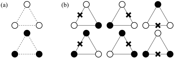
### Visual Description
\n
## Diagram: Network Structures
### Overview
The image presents two diagrams, labeled (a) and (b), depicting network structures composed of nodes and edges. Diagram (a) shows a single triangular network, while diagram (b) displays a repeating pattern of triangular networks connected to form a larger structure. Nodes are represented by circles, with some circles filled in black. Some nodes in diagram (b) are marked with an 'x'.
### Components/Axes
There are no explicit axes or scales. The diagrams are purely structural representations. The components are:
* **Nodes:** Represented by circles.
* **Edges:** Represented by lines connecting the nodes.
* **Node Color:** White or Black.
* **Node Marker:** 'x' (present only in diagram b).
### Detailed Analysis or Content Details
**Diagram (a):**
* The diagram consists of six nodes arranged in a triangular pattern.
* Three nodes are white circles, positioned at the vertices of an equilateral triangle.
* Three nodes are black circles, positioned similarly to the white circles, forming a second triangle offset from the first.
* Dashed lines connect each white node to its nearest black node, forming the edges of the network.
**Diagram (b):**
* The diagram consists of multiple triangular networks arranged in a repeating pattern.
* Each triangular network is composed of three white circles and three black circles, similar to diagram (a).
* Nodes are connected by solid lines.
* Several nodes are marked with an 'x'. These 'x' marked nodes are all white circles.
* The pattern appears to be a tessellation of triangular networks.
* The arrangement is roughly rectangular, with approximately 16 nodes visible.
* The 'x' markers appear to be placed on nodes that are not directly connected to other nodes within the immediate triangular structure.
### Key Observations
* Diagram (b) builds upon the structure of diagram (a), extending it into a larger, repeating network.
* The black and white nodes in both diagrams appear to alternate in position.
* The 'x' markers in diagram (b) highlight specific nodes within the network, potentially indicating a different status or role.
* The dashed lines in diagram (a) versus the solid lines in diagram (b) suggest a difference in the type or strength of connection.
### Interpretation
The diagrams likely represent abstract networks or relationships. The use of different node colors (black and white) could signify different types of entities or states. The 'x' markers in diagram (b) might indicate nodes that are isolated or have a specific function within the network. The change from dashed lines in (a) to solid lines in (b) could represent a strengthening or formalization of connections.
The diagrams could be used to model various systems, such as:
* **Social networks:** Nodes representing individuals, edges representing relationships.
* **Communication networks:** Nodes representing devices, edges representing communication links.
* **Biological networks:** Nodes representing genes or proteins, edges representing interactions.
* **Abstract mathematical structures:** Representing graphs or lattices.
Without further context, it is difficult to determine the precise meaning of the diagrams. However, the visual structure suggests a focus on connectivity, relationships, and potentially, the identification of key nodes or patterns within the network. The diagrams are not providing quantitative data, but rather a qualitative representation of network structure.
</details>
indicated by the crosses in Fig. 9 (b). This situation is called frustration. In the homogeneous antiferromagnetic Ising spin systems on lattices based on triangle such as triangular lattice and kagom´ e lattice, frustration appears in all triangles. Since such frustration comes from lattice geometry, this is called geometrical frustration. It should be noted that the homogeneous antiferromagnetic Ising spin systems on square lattice and hexagonal lattice have no frustration. Since these systems are bipartite systems which can be decomposed by two sublattices, these systems can be transformed on the ferromagnetic systems by local gauge transformation of all spins belonging to one of the sublattices.
Frustration appears in also inhomogeneous systems as shown in Fig. 10. The squares pointed by stars in Fig. 10 represent frustration plaquettes which are satisfied following relation:
$$k _ { k } = \sum _ { i , j \in O _ { k } } J _ { ij } < 0 ,$$
where /square k indicates the smallest square plaquette at the position k . If κ k for all k is positive, the system is not frustrated.
In general, frustration prevents the system from conventional magnetic ordering such as ferromagnetic order and N´ eel order, since there is no state where all interactions are satisfied energetically in frustrated systems. Frustration makes peculiar density of states which induces unconventional phase transition and slow dynamics. 112,115,135-144 Although many optimization problems can be represented by the Ising model with random interactions and magnetic fields, here we focus on the frustration effect which comes
Fig. 10. A ground state of the Ising spin system with random interactions. The dotted and solid lines represent ferromagnetic and antiferromagnetic interactions, respectively. The open and solid circles are the +1-state and the -1-state, respectively. The stars and crosses indicate frustration plaquettes and unfavorable interactions, respectively.
<details>
<summary>Image 10 Details</summary>
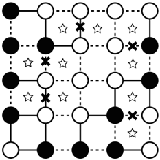
### Visual Description
\n
## Diagram: Grid-Based Pattern with Symbols
### Overview
The image depicts a 6x6 grid of circles, with varying fill colors (black and white) and additional symbols (stars and 'x' marks) overlaid on the grid. The grid is defined by dashed lines, creating a clear structure. There are no explicit axis labels or legends. The diagram appears to represent a pattern or arrangement of elements, potentially illustrating a state or configuration within a system.
### Components/Axes
The diagram consists of:
* **Grid:** A 6x6 arrangement of points connected by dashed lines.
* **Circles:** Circles are the primary elements, filled either black or white.
* **Stars:** Small star-shaped symbols are scattered across the grid.
* **'X' Marks:** 'X' shaped symbols are also scattered across the grid.
* **Lines:** Dashed lines form the grid structure.
### Detailed Analysis or Content Details
The grid can be described row by row, starting from the top:
* **Row 1:** Black, White, White, White, White, Black. Star, Star, 'X', Star, Star.
* **Row 2:** Black, White, White, White, Black, Black. Star, 'X', Star, Star, 'X'.
* **Row 3:** Black, White, White, Black, White, Black. Star, Star, Star, Star, Star.
* **Row 4:** Black, White, White, White, Black, White. Star, 'X', Star, Star, 'X'.
* **Row 5:** Black, White, Black, White, White, White. Star, Star, Star, Star, Star.
* **Row 6:** White, Black, Black, Black, White, White. 'X', Star, Star, Star, Star.
The arrangement of black and white circles does not appear to follow a simple, repeating pattern. The stars and 'X' marks are also distributed seemingly randomly, though they are not uniformly distributed.
### Key Observations
* The number of black circles is approximately equal to the number of white circles. (Roughly 18 of each).
* The 'X' marks appear less frequently than the stars. (4 'X' marks vs 16 stars).
* There is no obvious symmetry in the arrangement of the elements.
* The stars and 'X' marks are always placed *on* the grid intersections, not within the circles.
### Interpretation
This diagram likely represents a state or configuration within a system, possibly a network or a game board. The black and white circles could represent different states (e.g., on/off, active/inactive). The stars and 'X' marks could represent specific events, markers, or constraints within the system.
The lack of a clear pattern suggests that the system is either complex, stochastic (random), or governed by rules that are not immediately apparent from the diagram alone. The uneven distribution of the 'X' marks might indicate that certain events are rarer or more significant than others.
Without additional context, it is difficult to determine the precise meaning of the diagram. It could represent a cellular automaton, a game state (like a simplified version of Go or Reversi), or a visualization of a network with certain nodes highlighted. The diagram is a static snapshot, and understanding its dynamic behavior would require additional information. It is a visual representation of data, but the data itself is abstract and requires further interpretation.
</details>
from non-random interactions. In terms of statistical physics, this is a firststep study to investigate similarities and differences between thermal fluctuation and quantum fluctuation for frustrated systems. Furthermore, it is important topic for the optimization problems to consider the thermal fluctuation and quantum fluctuation effects for frustrated systems. To obtain the ground state of frustrated systems is to find how to put the unsatisfied bonds represented by the crosses. Since the unsatisfied bonds are regarded as some kind of constraints, this situation is similar with the traveling salesman problem in which there are some constraints as mentioned before. We explain two topics in this section. In the first half, we consider the order by disorder effect in fully-frustrated systems. In the last half, we explain non-monotonic dynamics in decorated bond systems.
## 5.2.1. Thermal Fluctuation and Quantum Fluctuation Effect of Geometrical Frustrated Systems
In general, there are many degenerated ground states in geometrical frustrated systems such as triangular antiferromagnetic Ising spin systems and kagom´ e antiferromagnetic Ising spin systems. In these cases, non-zero residual entropy which is entropy at zero temperature exists. Typical configurations of ground states of the triangular antiferromagnetic Ising spin systems are shown in Fig. 11. The residual entropy per spin of this system is S (tri) res /similarequal 0 . 323 k B , 145-148 where k B is the Boltzmann constant. Since the total entropy per spin is k B ln 2 /similarequal 0 . 693 k B , 46 . 6% of the total entropy remains even at zero temperature. In other words, there are macroscopic degenerated ground states in this system. In the antiferromagnetic Ising spin system on kagom´ e lattice, there are also macroscopic degenerated ground states. The residual entropy per spin of this system is S (kag) res /similarequal 0 . 502 k B , which is 72 . 4% of the total entropy. 149
Suppose we apply the simulated annealing or the quantum annealing with slow schedule for geometrical frustrated spin systems. Since there are macroscopically degenerated ground states in these systems, our purpose is to clarify whether all ground states are obtained with the same probabilities or biased probabilities. We first consider the obtained ground states in the case of the simulated annealing with slow schedule. If we decrease temperature slow enough, the obtained state should satisfy the equilibrium probability distribution. When the temperature is k B T /lessmuch | J | , the equilibrium probabilities of the ground states are dominant and that of any excited states can be neglected. The principle of equal weight which is the keystone in the equilibrium statistical physics says that if the eigenenergies of the
Fig. 11. Typical configurations of ground states of antiferromagnetic Ising spin system on triangular lattice. The open and solid circles are the +1-state and the -1-state, respectively. The dotted circles indicate free spin where the molecular field is zero.
<details>
<summary>Image 11 Details</summary>
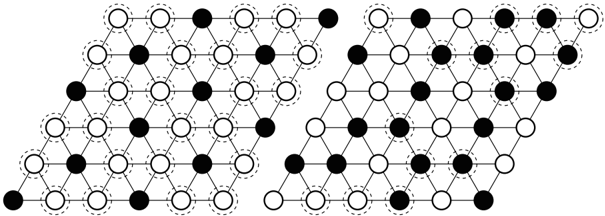
### Visual Description
\n
## Diagram: Hexagonal Lattice with Directed Edges
### Overview
The image depicts a hexagonal lattice structure composed of interconnected nodes (circles). Some nodes are filled black, while others are outlined only. Directed arrows connect the nodes, indicating a flow or relationship between them. The lattice appears to be truncated, forming a roughly triangular shape.
### Components/Axes
There are no explicit axes or labels in the traditional sense. The diagram consists of:
* **Nodes:** Circles, either filled black or outlined.
* **Edges:** Directed arrows connecting the nodes.
* **Lattice Structure:** A repeating hexagonal pattern.
### Detailed Analysis or Content Details
The diagram consists of a hexagonal lattice. The nodes are arranged in rows, with the number of nodes in each row increasing and then decreasing. The leftmost node is black. The nodes alternate between black and white (outlined) in a regular pattern within each row.
The directed arrows point predominantly to the right, with some pointing diagonally upwards to the right. The arrows are not present on every edge, and their presence seems to follow a pattern. The arrows are dashed.
Let's attempt to quantify the structure:
* **Rows:** Approximately 10 rows are visible.
* **Nodes per Row:** The number of nodes per row increases from 1 to approximately 8, then decreases back to 1.
* **Total Nodes:** Approximately 50-60 nodes are visible.
* **Black Nodes:** Approximately 25-30 nodes are black.
* **White Nodes:** Approximately 20-30 nodes are white (outlined).
* **Arrows:** Approximately 40-50 arrows are visible. The arrows are not uniformly distributed.
The pattern of arrows is as follows:
* Arrows are present on edges connecting black nodes to white nodes.
* Arrows are present on edges connecting white nodes to black nodes.
* Arrows are not present on edges connecting nodes of the same color.
### Key Observations
* The lattice structure is not perfectly regular; there is some truncation on the right side.
* The alternating pattern of black and white nodes suggests a binary state or classification.
* The directed arrows indicate a flow or relationship between nodes, potentially representing a process or network.
* The absence of arrows between nodes of the same color suggests a constraint or rule governing the flow.
### Interpretation
This diagram likely represents a state transition diagram or a network flow model. The black and white nodes could represent different states or categories, and the directed arrows could represent transitions between these states. The hexagonal lattice structure suggests a spatial or relational context.
The pattern of arrows indicates that transitions are only allowed between nodes of different states. This could represent a system where a change in state requires an interaction or exchange. The truncation of the lattice suggests that the system is either finite or that the diagram only shows a portion of a larger, infinite system.
The diagram could be used to model various phenomena, such as:
* A chemical reaction network
* A social network with directed relationships
* A computational model with state transitions
* A physical system with energy flow
Without additional context, it is difficult to determine the specific meaning of the diagram. However, the structure and patterns suggest a well-defined system with specific rules governing its behavior. The diagram is a visual representation of a complex system, and its interpretation requires a deeper understanding of the underlying principles.
</details>
microscopic state Σ A and Σ B are the same, the equilibrium probability of Σ A and that of Σ B are also the same. Then we obtain all macroscopic degenerated ground states with the same probability after the simulated annealing with slow schedule.
Next we consider the obtained ground states in the case of the quantum annealing where the transverse field decreases slow enough. Here we assume that the initial state is set to be the ground state of the Hamiltonian at the initial time. In order to capture the feature of the ground states in a graphical way, it is convenient to introduce the concept of free spin where the molecular field is zero. The molecular field at the i -th site is given by
$$h _ { i } ^ { ( eff ) } = \sum _ { j } ^ { ' } o _ { j } ^ { 2 }$$
where the summation runs over the nearest-neighbor sites of the i -th site. For instance, in Fig. 11, spins indicated by dotted circles are free spins. Here, the transverse field is expressed as
$$\sum _ { i = 1 } ^ { n } \sigma _ { i } ^ { - 1 } - \sum _ { i = 1 } ^ { n } ( \sigma _ { i } + 1 )$$
where ˆ σ + i and ˆ σ -i denote the raising and lowering operators at the i -th site, respectively. They are defined by
$$\sigma ^ { + } = ( 0 , 1 ) , \sigma ^ { - } = ( 0 , 0 ) .$$
The x -component of the Pauli matrix corresponds to the operator which flips the considered spin:
$$\sigma ^ { 2 } ( t ) = \langle t \rangle , \sigma ^ { 2 } ( t ) =$$
From this, the states which have large number of free spins are expected to become stable at the limit of Γ → 0+ and T = 0. Actually, in the adiabatic limit, the amplitudes of the states which have the maximum number of free spins are larger than the others. 150-154 When we decrease the transverse field slow enough, the state at each time can be well approximated by the ground state of the instantaneous Hamiltonian. Then we obtain specific ground states with high probability after the quantum annealing with slow schedule.
In this section, we considered the thermal fluctuation effect and the quantum fluctuation effect in the adiabatic limit. The simulated annealing can obtain all the ground states with the same probability, while on the other hand, the quantum annealing can obtain specific ground states in this limit. The biased probability distribution can be explained by the character of the quantum Hamiltonian. The selected states should depend on how to choice the quantum Hamiltonian. When we adopt the exchange type interaction as the quantum field, the states that have the maximum value of the 'free spin pair' should be selected. Moreover, it is an interesting topic to investigate differences between the simulated annealing and the quantum annealing with finite speed not only in terms of the quantum annealing but also in nonequilibrium statistical physics and condensed matter physics. At the present stage, to consider dynamic phenomena in strongly correlated systems is difficult, since a small number of theoretical methods for obtaining dynamic phenomena have been developed. If the technology of the artificial lattices develops more than ever, real-time dynamics and time-dependent phenomena of frustrated spin systems can be observed in real experiments.
## 5.2.2. Non-Monotonic Behavior of Correlation Function in Decorated Bond System
In the ferromagnetic Ising spin systems, the correlation function behaves monotonic against the temperature and transverse field. However, the behavior of the correlation function is non-monotonic as a function of temperature in some frustrated spin systems. As an example of non-monotonic correlation function, we introduce equilibrium properties of the correlation function in decorated bond systems in which the frustration exists. The Hamiltonian of the decorated bond systems where the number of system
spins is two shown in Fig. 12 is given by
$$H = - J _ { dir } ^ { 0 } \sigma _ { z } ^ { 2 } - J \sum _ { i = 1 } ^ { N d } s _ { i } ^ { z } ( σ _ { i } + σ _ { j } ) ,$$
where σ z i = ± 1 and s z i = ± 1 are, respectively, called system spins and decorated spins, and N d is the number of decorated spins. The circles and the squares in Fig. 12 represent the system spins and the decorated spins, respectively.
When the direct interaction between system spins J dir is zero and the decorated bond J is positive, the correlation function between system spins 〈 σ z 1 σ z 2 〉 is always positive and monotonic decaying function against the temperature. When the direct interaction between system spins J dir is negative and the decorated bond J is zero, on the other hand, the correlation function 〈 σ z 1 σ z 2 〉 is always negative and monotonic increasing function against the temperature. From this, the correlation function 〈 σ z 1 σ z 2 〉 is expected to behave non-monotonic in some cases for negative J dir and positive J or positive J dir and negative J . In order to obtain temperature dependence of the correlation function between system spins, we trace over spin states except the system spins:
$$T _ { r } ( s ; j ) e ^ { - B H } = A e K _ { e r t o i ^ { 2 } }$$
where A is just a constant which does not affect any physical quantities and the effective coupling K eff is given by
$$K _ { dir } = \frac { N d } { 2 } I n \cos h ( 2 \beta J ) +$$
Temperature dependence of the correlation function between system spins
Fig. 12. Decorated bond system where the number of system spins is two and the number of decorated spins is four ( N d = 4). The circles and squares represent system spins and decorated spins, respectively. The dotted and solid lines indicate the direct interaction between system spins and the decorated bonds, respectively.
<details>
<summary>Image 12 Details</summary>
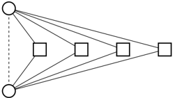
### Visual Description
\n
## Diagram: Network/Flow Representation
### Overview
The image depicts a diagram representing a network or flow between two sets of nodes. There are two circular nodes on the left and four square nodes on the right, connected by multiple lines. The diagram appears to illustrate a many-to-many relationship or a divergent flow.
### Components/Axes
The diagram consists of:
* **Circular Nodes (Input/Source):** Two circular nodes positioned on the left side of the diagram.
* **Square Nodes (Output/Destination):** Four square nodes positioned on the right side of the diagram.
* **Connecting Lines:** Lines connecting each circular node to each square node.
* **Dashed Line:** A dashed vertical line connecting the two circular nodes.
There are no axis titles, legends, or numerical values present in the image.
### Detailed Analysis or Content Details
The diagram shows a complete connection between the two circular nodes and the four square nodes. Each circular node is connected to each of the four square nodes via a straight line. The dashed line between the two circular nodes suggests a relationship or dependency between them.
Specifically:
* Circular Node 1 connects to Square Node 1, Square Node 2, Square Node 3, and Square Node 4.
* Circular Node 2 connects to Square Node 1, Square Node 2, Square Node 3, and Square Node 4.
### Key Observations
The diagram demonstrates a fully connected network where each input node influences all output nodes. The dashed line suggests a potential correlation or shared characteristic between the two input nodes. The absence of any labels or values makes it difficult to determine the nature of the relationship or the significance of the connections.
### Interpretation
The diagram likely represents a system where two sources (circular nodes) contribute to four outcomes (square nodes). The complete connectivity suggests that both sources have an impact on all outcomes. The dashed line could indicate that the two sources are related or operate in tandem. Without further context, it's difficult to determine the specific meaning of the diagram. It could represent a decision-making process, a data flow, or a network of relationships. The diagram is abstract and relies on the viewer to interpret the meaning based on the context in which it is presented. It is a visual representation of a many-to-many mapping.
</details>
is represented by using K eff :
$$C ^ { ( 0 ) } ( T ) = ( \sigma _ { i } ^ { 2 } j _ { 2 } ) = \frac { T _ { r } j _ { 2 } ^ { 3 } e ^ { - \beta H } } { T _ { r } e ^ { - \beta H } } = \frac { tanh K _ { eff } } { ( 156 ) }$$
Hereafter we set J as the energy unit and J is positive. In order to compare the effect of the direct interaction J dir fairly, we assume the form such as J dir = -xN d J . This is because the effective coupling K eff is proportional to the number of decorated spins N d under the assumption.
Figure 13 shows temperature dependence of correlation function between the system spins for N d = 1 and N d = 10 for several x . For small x and large x , the correlation function C (c) ( T ) is monotonic decreasing and increasing functions, respectively, against the temperature. However, the correlation function C (c) ( T ) behaves non-monotonic as a function of temperature for intermediate x . At the temperatures where the effective coupling K eff is larger than the critical value of the ferromagnetic Ising spin system on square lattice 19 K (square) c = 1 2 ln(1 + √ 2), ferromagnetic phase appears. On the other hand, at the temperature where K eff is less than -K (square) c , antiferromagnetic phase appears. In this case, successive
Fig. 13. The correlation function between system spins C (c) ( T ) as a function of temperature for N d = 1 (left panel) and for N d = 10 (right panel) in the cases of x = 0 . 1, 0 . 2, 0 . 5, 1 . 0, and 2 . 0.
<details>
<summary>Image 13 Details</summary>
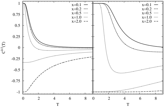
### Visual Description
## Chart: C<sup>(e)</sup>(T) vs. T for varying x
### Overview
The image presents a line chart displaying the relationship between C<sup>(e)</sup>(T) and T for different values of 'x'. The chart is divided into two panels, likely representing different conditions or perspectives on the same data. Each panel contains five lines, each corresponding to a specific 'x' value.
### Components/Axes
* **X-axis:** Labeled "T", ranging from approximately 0 to 8. The scale appears linear.
* **Y-axis:** Labeled "C<sup>(e)</sup>(T)", ranging from approximately -1 to 0.8. The scale appears linear.
* **Legend:** Located in the top-right corner of each panel, listing the 'x' values and their corresponding line styles:
* x = 0.1 (solid line)
* x = 0.2 (dashed line)
* x = 0.5 (dotted line)
* x = 1.0 (dash-dot line)
* x = 2.0 (long dash-dot line)
### Detailed Analysis or Content Details
**Panel 1 (Left):**
* **x = 0.1 (solid line):** Starts at approximately 0.75, rapidly decreases to around 0.1 at T=1, and then slowly approaches 0 as T increases.
* **x = 0.2 (dashed line):** Starts at approximately 0.5, decreases to around -0.1 at T=1, and then plateaus around -0.1 to -0.2 for higher T values.
* **x = 0.5 (dotted line):** Starts near 0.2, decreases to approximately -0.25 at T=1, and then remains relatively constant around -0.25 to -0.3.
* **x = 1.0 (dash-dot line):** Starts near 0, decreases to approximately -0.5 at T=1, and then continues to decrease, reaching around -0.75 at T=8.
* **x = 2.0 (long dash-dot line):** Starts near 0, decreases rapidly to approximately -1 at T=1, and remains close to -1 for higher T values.
**Panel 2 (Right):**
* **x = 0.1 (solid line):** Starts at approximately 0.75, rapidly decreases to around 0.1 at T=1, and then slowly approaches 0 as T increases.
* **x = 0.2 (dashed line):** Starts at approximately 0.5, decreases to around -0.1 at T=1, and then plateaus around -0.1 to -0.2 for higher T values.
* **x = 0.5 (dotted line):** Starts near 0.2, decreases to approximately -0.25 at T=1, and then remains relatively constant around -0.25 to -0.3.
* **x = 1.0 (dash-dot line):** Starts near 0, decreases to approximately -0.5 at T=1, and then continues to decrease, reaching around -0.75 at T=8.
* **x = 2.0 (long dash-dot line):** Starts near 0, decreases rapidly to approximately -1 at T=1, and remains close to -1 for higher T values.
The two panels appear to be identical.
### Key Observations
* As 'x' increases, the initial value of C<sup>(e)</sup>(T) tends to decrease.
* For all 'x' values, C<sup>(e)</sup>(T) generally decreases as T increases, especially in the initial range (T=0 to T=1).
* The rate of decrease varies with 'x'; higher 'x' values exhibit a more rapid initial decrease.
* For x = 2.0, C<sup>(e)</sup>(T) quickly reaches and remains near -1.
* The lines for x=0.1, x=0.2, and x=0.5 appear to converge as T increases.
### Interpretation
The chart likely represents a system where C<sup>(e)</sup>(T) is a function of temperature (T) and a parameter 'x'. The parameter 'x' could represent a concentration, a scaling factor, or another relevant variable in the system. The two panels being identical suggests that the system's behavior is consistent across different experimental setups or conditions.
The decreasing trend of C<sup>(e)</sup>(T) with increasing T suggests a process where the quantity represented by C<sup>(e)</sup>(T) is consumed or diminished as temperature rises. The different curves for varying 'x' indicate that the rate and extent of this consumption are influenced by the value of 'x'.
The convergence of the curves for lower 'x' values at higher temperatures suggests that the system reaches a state where the influence of 'x' becomes less significant. The rapid decrease and stabilization at -1 for x=2.0 could indicate a saturation effect or a complete consumption of the quantity represented by C<sup>(e)</sup>(T) at higher 'x' values.
Without further context, it's difficult to determine the specific physical or chemical process being modeled. However, the chart provides valuable insights into the relationship between C<sup>(e)</sup>(T), T, and 'x', and could be used to optimize or control the system's behavior.
</details>
phase transitions such as paramagnetic → antiferromagnetic → paramagnetic → ferromagnetic phases occur. Such phase transitions are called reentrant phase transitions which are sometimes appeared in frustrated systems. 115,139,155-160
We consider transverse field response of the decorated bond systems in the ground state. The Hamiltonian of the decorated bond system with transverse field is expressed as
$$H = - J _ { di } \sigma ^ { z } i σ _ { j } + \sum _ { i = 1 } ^ { N _ { d } } s _ { i } ( \sigma _ { i } + o _ { i } )$$
where ˆ s α i denotes the α -component of the Pauli matrix of the i -th decorated spin. Here we consider transverse-field dependence of the correlation function in the ground state given by
$$( g s ) ( T ) , \quad ( 1 5 8 )$$
where | ψ (gs) (Γ) 〉 denotes the ground state at the transverse field Γ. Figure 14 shows transverse-field dependence of C (q) (Γ) for N d = 1 and N d = 10 for several x .
Fig. 14. The correlation function between system spins C (q) (Γ) as a function of transverse field for N d = 1 (left panels) and for N d = 10 (right panels) in the cases of x = 0 . 1, 0 . 2, 0 . 5, 1 . 0, and 2 . 0.
<details>
<summary>Image 14 Details</summary>
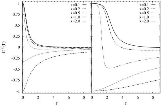
### Visual Description
\n
## Chart: Correlation Function vs. Gamma
### Overview
The image presents a chart displaying the correlation function, C<sup>(ω)</sup>(Γ), as a function of Gamma (Γ) for different values of 'x'. The chart is split into two panels, likely representing different conditions or scales. Each panel shows five curves, each corresponding to a specific 'x' value.
### Components/Axes
* **X-axis:** Gamma (Γ), ranging from approximately 0 to 8.
* **Y-axis:** Correlation Function C<sup>(ω)</sup>(Γ), ranging from approximately -1 to 0.75.
* **Legend:** Located in the top-right corner of each panel, listing the 'x' values and their corresponding line styles:
* x = 0.1 (solid line)
* x = 0.2 (dashed line)
* x = 0.5 (dotted line)
* x = 1.0 (dash-dot line)
* x = 2.0 (long dash-dot line)
### Detailed Analysis
The chart consists of two identical panels, side-by-side. We will analyze one panel and assume the other exhibits the same trends.
**Left Panel:**
* **x = 0.1 (solid line):** Starts at approximately 0.6, rapidly decreases to around 0.1 at Γ ≈ 1, and then plateaus around 0.05 for Γ > 2.
* **x = 0.2 (dashed line):** Starts at approximately 0.3, decreases more gradually than x=0.1, reaching around 0 at Γ ≈ 3, and remains near 0 for larger Γ.
* **x = 0.5 (dotted line):** Starts at approximately 0.1, decreases to a minimum of around -0.25 at Γ ≈ 2, and then slowly increases, approaching 0 for Γ > 6.
* **x = 1.0 (dash-dot line):** Starts at approximately -0.1, decreases to a minimum of around -0.5 at Γ ≈ 2, and then slowly increases, approaching 0 for Γ > 6.
* **x = 2.0 (long dash-dot line):** Starts at approximately -0.3, rapidly decreases to a minimum of around -1 at Γ ≈ 1, and then slowly increases, approaching 0 for Γ > 6.
**Right Panel:**
The trends in the right panel are identical to those in the left panel.
### Key Observations
* The curves exhibit significant changes in behavior around Γ ≈ 1-2.
* Higher values of 'x' generally lead to more negative correlation function values, especially at lower Γ.
* For all 'x' values, the correlation function tends to approach 0 as Γ increases.
* The solid line (x=0.1) remains positive throughout the range of Γ, while the other lines become negative.
### Interpretation
This chart likely represents the correlation function in a physical system, possibly a plasma or a condensed matter system. The parameter 'x' could represent a control parameter such as density or interaction strength. The Gamma (Γ) parameter could represent a frequency or a damping rate.
The fact that the correlation function becomes negative for higher 'x' values suggests a transition to a state with anti-correlation. The rapid changes around Γ ≈ 1-2 could indicate a resonance or instability in the system. The approach to zero correlation at high Γ suggests that the system becomes more disordered or that correlations are screened out at higher frequencies or damping rates.
The two panels being identical suggests that the observed behavior is consistent and not dependent on specific experimental conditions. The chart provides insights into the collective behavior of the system and how it changes with the control parameter 'x'. The negative correlation for higher x values is a particularly interesting feature, potentially indicating a change in the fundamental nature of the interactions within the system.
</details>
For small x and large x , the correlation function C (q) (Γ) behaves monotonic decreasing and increasing, respectively as a function of transverse field, whereas for intermediate x , transverse-field dependence of the correlation function behaves nonmonotonic as well as the case of thermal fluctuation. Then, the reentrant phase transition also occurs by changing the transverse field. However there is a difference between the thermal fluctuation effect and the quantum fluctuation effect for decorated bond system. The temperature where C (c) ( T ) = 0 is satisfied is the same when we change the number of decorated spins N d , whereas the transverse field at C (q) (Γ) = 0 is different when N d is changed.
The thermal fluctuation and the quantum fluctuation have similar properties for the phase transition phenomena in general. Indeed, the reentrant phase transitions occur by changing the thermal fluctuation and also the quantum fluctuation as shown in this section. However as described in Sec. 5.1, in order to obtain the best solution of optimization problems, it is better to erase phase transition. By dealing with thermal and quantum fluctuation effects for frustrated systems exhaustively, we can construct the best form of the adding fluctuation which erases phase transition e .
## 6. Conclusion
In this paper, we described some aspects of the quantum annealing from viewpoints of statistical physics, condensed matter physics, and computational physics. Originally, the quantum annealing has been proposed as a method which can solve efficiently optimization problems in a generic way. Since many optimization problems can be mapped onto the Ising model or generalized Ising model such as the clock model and the Potts model, it has been considered that we can obtain a better solution by using methods which were developed in computational physics. For instance, we can obtain a better solution by decreasing temperature (thermal fluctuation) gradually in the simulated annealing which is one of the most famous practical methods. In the quantum annealing, we decrease an introduced quantum field (quantum fluctuation) instead of temperature (thermal fluctuation). In many studies, it was reported that a better solution can be obtained
e It is not necessary that the adding fluctuation is restricted in quantum physics. From a viewpoint of optimization problems, we can arbitrary form adding term. Furthermore, it has studied that other novel fluctuation which may be able to erase phase transition as an alternative to thermal and quantum fluctuations. 14,116,161,162 Of course, if we want to realize experimentally, it is better that the added fluctuation term should be some kind of quantum fluctuation.
by the quantum annealing efficiently in comparison with the simulated annealing as we explained in Sec. 4. Thus, the quantum annealing method is expected to be a generic and powerful solver of optimization problems as an alternative to the simulated annealing.
The quantum annealing has become a milestone of some related fields under the situation in which the quantum annealing itself has been studied exhaustively. Since we use the quantum fluctuation in the quantum annealing with ingenuity, to obtain a better solution by using the quantum annealing is a kind of quantum information processing. Thus, many implementation methods of the quantum annealing in theoretical and experimental ways have been proposed by many researchers. A number of theoretical implementation methods are proposed based on knowledge of statistical physics. As we shown in Sec. 5, question of what are differences between the simulated annealing and the quantum annealing and question of which is efficient in the given optimization problem are catalysts to investigate differences between the thermal fluctuation and the quantum fluctuation in a deeper way. On top of that, studies on the quantum annealing are expected to open the door to consider equilibrium and nonequilibrium statistical physics. Recently, preparation methods of intended Hamiltonian have been established in some experimental systems such as artificial lattices and nuclear magnetic resonance because of recent development of experimental techniques. As long as we use classical computer and our present knowledge, there are a huge number of problems where to obtain the best solution is difficult without any and every approximation in theoretical methods. However if we prepare the Hamiltonian which expresses our intended problem, we can calculate experimentally the stable state of the prepared Hamiltonian in near future.
The quantum annealing transcends just a method for obtaining the best solution of optimization problems and it will make a development in wide area of science. Although it seems that studies on the quantum annealing itself have been well established, we believe that the quantum annealing plays a role as a bridge with the abovementioned area of science and the quantum information.
## Acknowledgement
The authors are grateful to Bernard Barbara, Bikas K. Charkrabarti, Naomichi Hatano, Masaki Hirano, Naoki Kawashima, Kenichi Kurihara, Yoshiki Matsuda, Seiji Miyashita, Hiroshi Nakagawa, Mikio Nakahara, Hidetoshi Nishimori, Masayuki Ohzeki, Hans de Raedt, Per Arne Rikvold,
Issei Sato, Sei Suzuki, Eric Vincent, and Yoshihisa Yamamoto for their valuable comments. S.T. acknowledges Keisuke Fujii, Yoshifumi Nakada, and Takahiro Sagawa for their useful discussion during the lecture. S.T. is partly supported by Grand-in-Aid for JSPS Fellows (23-7601). R.T. is partly supported financially by National Institute for Materials Science (NIMS). The computation in the present work was performed on computers at the Suprecomputer Center, Institute for Solid State Physics, University of Tokyo.
## References
1. S. Kirkpatrick, C. D. Gelatt Jr., and M. P. Vecchi, Science 220 , 671 (1983).
2. S. Kirkpatrick, J. Stat. Phys. 34 , 975 (1984).
3. S. Geman and D. Geman, IEEE Transactions on Pattern Analysis and Machine Intelligence 6 , 721 (1984).
4. A. B. Finnila, M. A. Gomez, C. Sebenik, C. Stenson, and J. D. Doll, Chem. Phys. Lett. 219 , 343 (1994).
5. T. Kadowaki and H. Nishimori, Phys. Rev. E 58 , 5355 (1998).
6. J. Brooke, D. Bitko, T. F. Rosenbaum, and G. Aeppli, Science 284 , 779 (1999).
7. E. Farhi, J. Goldstone, S. Gutmann, J. Lapan, A. Lundgren, and D. Preda, Science 292 , 472 (2001).
8. G. E. Santoro, R. Martoˇ n´ ak, E. Tosatti, and R. Car, Science 295 , 2427 (2002).
9. A. Das and B. K. Chakrabarti, Quantum Annealing and Related Optimization Methods (Springer, Heidelberg, 2005).
10. A. Das and B. K. Chakrabarti, Rev. Mod. Phys. 80 , 1061 (2008).
11. M. Ohzeki and H. Nishimori, J. Comp. and Theor. Nanoscience 8 , 963 (2011).
12. K. Kurihara, S. Tanaka, and S. Miyashita, Proceedings of the 25th Conference on Uncertainty in Artificial Intelligence (2009).
13. I. Sato, K. Kurihara, S. Tanaka, H. Nakagawa, and S. Miyashita, Proceedings of the 25th Conference on Uncertainty in Artificial Intelligence (2009).
14. S. Tanaka, R. Tamura, I. Sato, and K. Kurihara, to appear in Kinki University Quantum Computing Series: 'Summer School on Diversities in Quantum Computation/Information' .
15. C. Jarzynski, Phys. Rev. Lett. 78 , 2690 (1997).
16. C. Jarzynski, Phys. Rev. E 56 , 5018 (1997).
17. M. Ohzeki, Phys. Rev. Lett. 105 , 050401 (2010).
18. E. Ising, Z. Phys. 31 , 253 (1925).
19. L. Onsager, Phys. Rev. 65 , 117 (1944).
20. M. Blume, Phys. Rev. 141 , 517 (1966).
21. H. W. Capel, Phys. Lett. 23 , 327 (1966).
22. J. Tobochnik, Phys. Rev. B 26 , 6201 (1982).
23. M. S. S. Challa and D. P. Landau, Phys. Rev. B 33 , 437 (1986).
24. R. B. Potts, Proc. Cambridge Philos. Soc. 48 , 106 (1952).
25. F. Y. Wu, Rev. Mod. Phys. 54 , 235 (1982).
26. T. Ohtsuka, J. Phys. Soc. Jpn. 16 , 1549 (1961).
27. M. Rayl, O. E. Vilches, and J. C. Wheatley, Phys. Rev. 165 , 698 (1968).
28. K. ˆ Ono, M. Shinohara, A. Ito, N. Sakai, and M. Suenaga, Phys. Rev. Lett. 24 , 770 (1970).
29. N. Achiwa, J. Phys. Soc. Jpn. 27 , 561 (1969).
30. M. Mekata and K. Adachi, J. Phys. Soc. Jpn. 44 , 806 (1978).
31. A. H. Cooke, D. T. Edmonds, F. R. McKim, and W. P. Wolf, Proc. Roy. Soc. London Ser. A 252 , 246 (1959).
32. A. H. Cooke, D. T. Edmonds, C. B. P. Finn, and W. P. Wolf, Proc. Roy. Soc. London Ser. A 306 , 313 (1968).
33. A. H. Cooke, D. T. Edmonds, C. B. P. Finn, and W. P. Wolf, Proc. Roy. Soc. London Ser. A 306 , 335 (1968).
34. K. Takeda, M. Matsuura, S. Matsukawa, Y. Ajiro, and T. Haseda, Proc. 12th Int. Conf. Low Temp. Phys., Kyoto 803 (1970).
35. K. Takeda, S. Matsukawa, and T. Haseda, J. Phys. Soc. Jpn. 30 , 1330 (1971).
36. B. N. Figgis, M. Gerloch, and R. Mason, Acta. Crystallogr. 17 , 506 (1964).
37. R. F. Wielinga, H. W. J. Blote, J. A. Roest, and W. J. Huiskamp, Physica 34 , 223 (1967).
38. K. W. Mess, E. Lagendijk, D. A. Curtis, and W. J. Huiskamp, Physica 34 , 126 (1967).
39. G. R. Hoy and F. de S. Barros, Phys. Rev. 139 , A929 (1965).
40. M. Matsuura, H. W. J. Blote, and W. J. Huiskamp, Physica 50 , 444 (1970).
41. R. D. Pierce and S. A. Friedberg, Phys. Rev. B 3 , 934 (1971).
42. K. Takeda and S. Matsukawa, J. Phys. Soc. Jpn. 30 , 887 (1971).
43. E. Stryjewski and N. Giordano, Adv. Phys. 26 , 487 (1977).
44. D. J. Breed, K. Gilijamse, and A. R. Miedema, Physica 45 , 205 (1969).
45. K. ˆ Ono, A. Ito, and T. Fujita, J. Phys. Soc. Jpn. 19 , 2119 (1964).
46. R. J. Birgeneau, W. B. Yelon, E. Cohen, and J. Makovsky, Phys. Rev. B 5 , 2607 (1972).
47. J. C. Wright, H. W. Moos, J. H. Colwell, B. W. Magnum, and D. D. Thornton, Phys. Rev. B 3 , 843 (1971).
48. G. T. Rado, Phys. Rev. Lett. 23 , 644 (1969).
49. W. Scharenberg and G. Will, Int. J. Magnetism 1 , 277 (1971).
50. H. Fuess, A. Kallel, and F. Tch´ eou, Solid State Commun. 9 , 1949 (1971).
51. M. Ball, M. J. M. Leask, W. P. Wolf, and A. F. G. Wyatt, J. Appl. Phys. 34 , 1104 (1963).
52. J. C. Norvell, W. P. Wolf, L. M. Corliss, J. M. Hastings, and R. Nathans, Phys. Rev. 186 , 557 (1969).
53. J. C. Norvell, W. P. Wolf, L. M. Corliss, J. M. Hastings, and R. Nathans, Phys. Rev. 186 , 567 (1969).
54. G. A. Baker, Jr., Phys. Rev. 129 , 99 (1963).
55. M. F. Sykes, D. L. Hunter, D. S. McKenzie, and B. R. Heap, J. Phys. A: Gen. Phys. 5 , 667 (1972).
56. J. W. Stout and E. Catalano, J. Chem. Phys. 23 , 2013 (1955).
57. C. Domb and A. R. Miedema, Progress in low Temperature Physics, Vol. 4, edited by C. J. Gorter (North-Holland, Amsterdam, 1964).
58. G. K. Wertheim and D. N. E. Buchanan, Phys. Rev. 161 , 478 (1967).
59. Y. Shapira, Phys. Rev. B 2 , 2725 (1970).
60. M. A. Nielsen and I. L. Chuang, Quantum Computation and Quantum Information (Cambridge University Press, Cambridge, 2000).
61. M. Nakahara and T. Ohmi, Quantum Computing: From Linear Algebra to Physical Realizations (Taylor & Francis, London, 2008).
62. D. G. Cory, A. F. Fahmy, and T. F. Havel, Proc. Natl. Acad. Sci. USA 94 , 1634 (1997).
63. D. G. Cory, M. D. Price, W. Maas, E. Knill, R. Laflamme, W. H. Zurek, T. F. Havel, and S. S. Somaroo, Phys. Rev. Lett. 81 , 2152 (1998).
64. N. A. Gershenfeld and I. L. Chuang, Science 275 , 350 (1997).
65. I. L. Chuang, L. M. K. Vandersypen, X. Zhou, D. W. Leung, and S. Lloyd, Nature 393 , 143 (1998).
66. J. A. Jones and M. Mosca, J. Chem. Phys. 109 , 1648 (1998).
67. E. Knill, I. Chuang, and R. Laflamme, Phys. Rev. A 57 , 3348 (1998).
68. R. Laflamme, E. Knill, W. H. Zurek, P. Catasti, and S. V. S. Mariappan, Phil. Trans. R. Soc. Lond. A 356 , 1941 (1998).
69. J. A. Jones and M. Mosca, Phys. Rev. Lett. 83 , 1050 (1999).
70. M. D. Price, S. S. Somaroo, A. E. Dunlop, T. F. Havel, and D. G. Cory, Phys. Rev. A 60 , 2777 (1999).
71. L. M. K. Vandersypen, C. S. Yannoni, M. H. Sherwood, and I. L. Chuang, Phys. Rev. Lett. 83 , 3085 (1999).
72. L. M. K. Vandersypen, M. Steffen, G. Breyta, C. S. Yannoni, R. Cleve, and I. L. Chuang, Phys. Rev. Lett. 85 , 5452 (2000).
73. L. M. K. Vandersypen, M. Steffen, G. Breyta, C. S. Yannoni, M. H. Sherwood, and I. L. Chuang, Nature (London) 414 , 883 (2001).
74. M. Nakahara, Y. Kondo, K. Hata, and S. Tanimura, Phys. Rev. A 70 , 052319 (2004).
75. Y. Kondo, J. Phys. Soc. Jpn. 76 , 104004 (2007).
76. H. Suwa and S. Todo, Phys. Rev. Lett. 105 , 120603 (2010).
77. H. Suwa and S. Todo, arXiv :1106.3562.
78. R. H. Swendsen and J. S. Wang, Phys. Rev. Lett. 58 , 86 (1987).
79. U. Wolff, Phys. Rev. Lett. 62 , 361 (1989).
80. K. Hukushima and K. Nemoto, J. Phys. Soc. Jpn. 65 , 1604 (1996).
81. N. Kawashima and K. Harada, J. Phys. Soc. Jpn. 73 , 1379 (2004).
82. T. Nakamura, Phys. Rev. Lett. 101 , 210602 (2008).
83. S. Morita, S. Suzuki, and T. Nakamura, Phys. Rev. E 79 , 065701(R) (2009).
84. H. F. Trotter, Proc. Am. Math. Soc. 10 , 545 (1959).
85. M. Suzuki, Prog. Theor. Phys. 56 , 1454 (1976).
86. T. Kadowaki, Ph. D thesis, Tokyo Institute of Technology (1998).
87. K. Tanaka and T. Horiguchi, Electronics and Communications in Japan, Part 3: Fundamental Electronic Science 83 , 84 (2000).
88. K. Tanaka and T. Horiguchi, Interdisciplinary Information Science 8 , 33 (2002).
89. H. Attias, Proceedings of the 15th Conference on Uncertainly in Artificial Intelligence 21 (1999).
90. L. Landau, Phys. Z. Sowjetunion 2 , 46 (1932).
91. C. Zener, Proc. R. Soc. London Ser. A 137 , 696 (1932).
92. E. C. G. St¨ uckelberg, Helv. Phys. Acta 5 , 369 (1932).
93. N. Rosen and C. Zener, Phys. Rev. 40 , 502 (1932).
94. B. K. Chakrabarti, A. Dutta, and P. Sen, Quantum Ising Phases and Transitions in Transverse Ising Models (Springer Verlag, Berlin, 1996).
95. G. T. Trammel, J. Appl. Phys. 31 , 362S (1960).
96. A. H. Cooke, D. T. Edmonds, C. B. P. Finn, and W. P. Wolf, J. Phys. Soc. Jpn. 17 , Suppl. B1 481 (1962).
97. J. W. Stout and R. C. Chisolm, J. Chem. Phys. 36 , 979 (1962).
98. V. L. Moruzzi and D. T. Teaney, Sol. State. Comm. 1 , 127 (1963).
99. A. Narath and J. E. Schriber, J. Appl. Phys. 37 , 1124 (1966).
100. R. F. Wielinga and W. J. Huiskamp, Physica 40 , 602 (1969).
101. W. P. Wolf, J. Phys. (Paris) 32 Suppl. C1 26 (1971).
102. W. Wu, B. Ellman, T. F. Rosenbaum, G. Aeppli, and D. H. Reich, Phys. Rev. Lett. 67 , 2076 (1991).
103. W. Wu, D. Bitko, T. F. Rosenbaum, and G. Aeppli, Phys. Rev. Lett. 71 , 1919 (1993).
104. D. H. Reich, B. Ellman, J. Yang, T. F. Rosenbaum, G. Aeppli, and D. P. Belanger, Phys. Rev. B 42 , 4631 (1990).
105. T. F. Rosenbaum, J. Phys.: Condens. Matter 8 , 9759 (1996).
106. D. H. Reich, T. F. Rosenbaum, G. Aeppli, and H. Guggenheim, Phys. Rev. B 34 , 4956 (1986).
107. J. A. Mydosh, Spin Glasses: An Experimental Introduction (Taylor & Francis, London, 1993).
108. P. Bak, C. Tang, and K. Wiesenfeld, Phys. Rev. Lett. 59 , 381 (1987).
109. R. Martoˇ n´ ak, G. E. Santoro, and E. Tosatti, Phys. Rev. E 70 , 057701 (2004).
110. S. Tanaka and S. Miyashita, J. Phys.: Condens. Matter 19 , 145256 (2007).
111. H. Takayama and K. Hukushima, J. Phys. Soc. Jpn. 76 , 013702 (2007).
112. S. Tanaka and S. Miyashita, J. Phys. Soc. Jpn. 76 , 103001 (2007).
113. S. Miyashita, S. Tanaka, and M. Hirano, J. Phys. Soc. Jpn. 76 , 083001 (2007).
114. S. Tanaka and S. Miyashita, J. Phys. Soc. Jpn. 78 , 084002 (2009).
115. S. Tanaka and S. Miyashita, Phys. Rev. E 81 , 051138 (2010), Virtual Journal of Quantum Information 10 , (2010).
116. S. Tanaka and R. Tamura, J. Phys.: Conf. Ser. 320 , 012025 (2011).
117. H. Nishimori and G. Ortiz, Elements of Phase Transitions and Critical Phenomena (Oxford Univ Press, Oxford, 2010).
118. N. Ito, M. Taiji, and M. Suzuki, J. Phys. Soc. Jpn. 56 , 4218 (1987).
119. T. W. B. Kibble, J. Phys. A 9 , 1387 (1976).
120. T. W. B. Kibble, Phys. Rep. 67 , 183 (1980).
121. W. H. Zurek, Nature (London) 317 , 505 (1985).
122. B. Damski, Phys. Rev. Lett. 95 , 035701 (2005).
123. W. H. Zurek, U. Dorner, and P. Zoller, Phys. Rev. Lett. 95 , 105701 (2005).
124. V. M. H. Ruutu, V. B. Eltsov, A. J. Gill, T. W. B. Kibble, M. Krusius, Y. G. Makhlin, B. Placais, G. E. Volovik, and W. Xu, Nature (London) 382 , 334 (1996).
125. V. B. Eltsov, T. W. B. Kibble, M. Krusius, V. M. H. Ruutu, and G. E. Volovik, Phys. Rev. Lett. 85 , 4739 (2000).
126. H. Saito, Y. Kawaguchi, and M. Ueda, Phys. Rev. A 76 , 043613 (2007).
127. C. N. Weiler, T. W. Neely, D. R. Scherer, A. S. Bradley, M. J. Davis, and B. P. Anderson, Nature (London) 455 , 948 (2008).
128. S. Suzuki, J. Stat. Mech. P03032 (2009).
129. S. Suzuki, J. Phys.: Conf. Ser. 302 , 012046 (2011).
130. R. J. Glauber, J. Math. Phys. 4 , 294 (1963).
131. R. Shankar and G. Murthy, Phys. Rev. B 36 , 536 (1987).
132. D. S. Fisher, Phys. Rev. B 51 , 6411 (1995).
133. J. Dziarmaga, Phys. Rev. B 74 , 064416 (2006).
134. G. Biroli, L. F. Cugliandolo, and A. Sicilia, Phys. Rev. E 81 , 050101(R) (2010).
135. G. Toulouse, Commun. Phys. (London) 2 , 115 (1977).
136. R. Liebmann, Statistical Mechanics of Periodic Frustrated Ising Systems (Springer-Verlag, Berlin/Heidelberg, GmbH, Heidelberg, 1986).
137. H. Kawamura, J. Phys.: Condens. Matter 10 , 4707 (1998).
138. H. T. Diep (ed.), Frustrated Spin Systems (World Scientific, Singapore, 2005).
139. S. Tanaka and S. Miyashita, Prog. Theor. Phys. Suppl. 157 , 34 (2005).
140. S. Tanaka and S. Miyashita, J. Phys. Soc. Jpn. 76 , 103001 (2007).
141. R. Tamura and N. Kawashima, J. Phys. Soc. Jpn. 77 , 103002 (2008).
142. S. Tanaka and S. Miyashita, J. Phys. Soc. Jpn. 78 , 084002 (2009).
143. R. Tamura and N. Kawashima, J. Phys. Soc. Jpn. 80 , 074008 (2011).
144. R. Tamura, N. Kawashima, T. Yamamoto, C. Tassel, and H. Kageyama, Phys. Rev. B 84 , 214408 (2011).
145. K. Husimi and I. Syozi, Prog. Theor. Phys. 5 , 177 (1950).
146. R. M. F. Houtappel, Physica 16 , 425 (1950).
147. G. H. Wannier, Phys. Rev. 79 , 357 (1950).
148. G. H. Wannier, Phys. Rev. B 7 , 5017 (1973).
149. K. Kano and S. Naya, Prog. Theor. Phys. 10 , 158 (1953).
150. Y. Matsuda, H. Nishimori, and H. G. Katzgraber, J. Phys.: Conf. Ser. 143 , 012003 (2009).
151. Y. Matsuda, H. Nishimori, and H. G. Katzgraber, New J. Phys. 11 , 073021 (2009).
152. S. Tanaka, M. Hirano, and S. Miyashita, Lecture Note in Physics 'Quantum Quenching, Annealing, and Computation' (Springer) 802 , 215 (2010).
153. S. Tanaka, to appear in proceedings of Kinki University Quantum Computing Series: 'Symposium on Quantum Information and Quantum Computing' (2011).
154. S. Tanaka and R. Tamura, in preparation .
155. E. H. Fradkin and T. P. Eggarter, Phys. Rev. A 14 , 495 (1976).
156. S. Miyashita, Prog. Theor. Phys. 69 , 714 (1983).
157. H. Kitatani, S. Miyashita, and M. Suzuki, Phys. Lett. 108A , 45 (1985).
158. H. Kitatani, S. Miyashita, and M. Suzuki, J. Phys. Soc. Jpn. 55 , 865 (1986).
159. P. Azaria, H. T. Diep, and H. Giacomini, Phys. Rev. Lett. 59 , 1629 (1987).
160. S. Miyashita and E. Vincent, Eur. Phys. J. B 22 , 203 (2001).
161. R. Tamura, S. Tanaka, and N. Kawashima, Prog. Theor. Phys. 124 , 381 (2010).
162. S. Tanaka and R. Tamura, and N. Kawashima, J. Phys.: Conf. Ser. 297 , 012022 (2011).