# Unknown Title
## On reasoning in networks with qualitative uncertainty
## Simon Parsons*and E. H. Mamdani
Department of Electronic Engineering,
Queen Mary and Westfield College, Mile End Road, London, E1 4NS, UK.
## Abstract
In this paper some initial work towards a new approach to qualitative reasoning under un certainty is presented. This method is not only applicable to qualitative probabilistic reasoning, as is the case with other methods, but also allows the qualitative propagation within networks of values based upon possi bility theory and Dempster-Shafer evidence theory. The method is applied to two simple networks from which a large class of directed graphs may be constructed. The results of this analysis are used to compare the quali tative behaviour of the three major quantita tive uncertainty handling formalisms, and to demonstrate that the qualitative integration of the formalisms is possible under certain as sumptions.
## 1 INTRODUCTION
In the past few years, the use of reasoning about qual itative changes in probability to deal with uncertainty has become widely accepted, being applied to domains such as planning [Wellman 1990b] and generating plau sible explanations [Henrion and Druzdzel 1990]. Such a qualitative approach has certain advantages over quantitative methods, not least among which is the ability to model domains in which the relation between variables is uncertain as a result of incomplete knowl edge, and domains in which numerical representations are inappropriate.
The existence of the latter, as Wellman [1990a] points out, is often due to the precision of numerical methods which can, in certain circumstances, lead to knowledge bases being applicable only in very narrow areas be cause of the interaction between values at a fine level of detail. Since they view the world at a higher level of abstraction, qualitative methods are immune to such
*Current address: Advanced Computation Laboratory, Imperial Cancer Research Fund, P. 0. Box 123, Lincoln's Inn Fields, London, WC2A 3PX, UK
problems; the small complications such interactions cause simply have no effect at the coarse level of detail with which qualitative methods are concerned.
The focus of the qualitative approach of Wellman and Henrion and Druzdzel is assessing the impact of evi dence. That is assessing how the change in probabil ity of one event due to some piece of evidence affects the probability of other events. For instance, taking a patient's temperature and finding that it is 38C is evidence that increases the probability that she has a fever, which in turn increases the probability that she has measles.
Now, when using the qualitative method we reason with a restricted set of values. Instead of using the full range of real numbers we are only interested in whether values are positive [+], negative [-], zero [0], or any of the three [?]. Thus we can determine that since the probability of fever increases, the change in prob ability is [+], and use this to decide that the change in probability of measles is also [+]. This is clearly weaker information than that obtained by traditional methods but may still be useful [Wellman 1990a], in particular since qualitative results may be obtained in situations where no numerical information may be de duced.
## 2 A NEW QUALITATIVE APPROACH
This paper presents a new approach to reasoning about qualitative changes. This work is drawn from the first author's thesis [Parsons 1993] in which may be found a number of extensions to the work described here. The motivation behind this work was to integrate dif ferent approaches to reasoning under uncertainty, in particular probability, possibility [Zadeh 1978] [Dubois and Prade 1988a], and evidence [Shafer 1976] [Smets 1988) theories. Thus, our qualitative approach differs from that described above in that it is concerned with changes in possibility values [Parsons 1992a] and belief values [Parsons 1992b) as well as probability values. As a result we need a general way of referring to values that may be probabilities, possibilities or beliefs.
Definition 2.1: The certainty value of a variable X taking value x, val(x), is either the probability of X, p( x), the possibility of X, II( x), or the belief in X, bel(x).
We set our work in the framework of singly connected networks in which the nodes represent variables of in terest, and the edges represent explicit dependencies between the variables. When the edges, of such graphs are quantified with conditional probability values they are similar to those studied by Pearl [1988], when pos sibility values are used the graphs are similar to those of Fonck and Straszecka [1991J and when belief values are used the graphs are those studied by Smets [ 1991 J .
Each node in a graph represents a binary valued vari able. The probability values associated with a vari able X which has possible values x and ·X are p(x) and p( ·x), and the possibility values associated with X are II(x) and II(·x). Belief values may be assigned to any subset of the values of X, so it is possible to have up to three beliefs associated with X; bel({x}), bel({·x}) and bel({x,·x}). For simplicity these will be written as bel(x), bel(·x) and bel(x U ·x). This rather restrictive framework is loosened in [Parsons 1993J where non-binary values and multiply connected are considered.
Wellman [ 1990a, 1990bJ and Henrion and Druzdzel [ 1990J base their work upon the premise that a suitable interpretation of "a positively influences c" is that:
$$( 1 ) ( 2 ) ( 3 )$$
This seems reasonable, but it is a premise; there are other ways of encoding the information that seem equally intuitively acceptable, for instance p( c I a) > p(c) and p(c I a) > p(·c I a) [Dubois and Prade 1991J. Since our aim was to provide a method that was suit able for integrating formalisms we wanted to start from first principles thus minimising the number of neces sary assumptions. As a result, a different approach was adopted as described below.
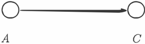
Given a link joining nodes A and C as in Figure 1, we are interested in the way in which a change in the value of a, say, expressed in a particular formalism, in fluences the value of c. Note that the arrow between A and C does not necessarily indicate a causal relation ship between them, rather it suggests that propagation of qualitative changes will be from A to C.
Figure 1: A simple network
<details>
<summary>Image 1 Details</summary>
### Visual Description
## Diagram: Process Flow from A to C
### Overview
The image depicts a simple directional diagram with two labeled circular nodes ("A" and "C") connected by a single arrow. The arrow originates from node A (left) and points toward node C (right), indicating a unidirectional relationship or process flow. No additional annotations, numerical data, or contextual elements are present.
### Components/Axes
- **Nodes**:
- **A**: Left circular node, labeled "A" in black text below the circle.
- **C**: Right circular node, labeled "C" in black text below the circle.
- **Arrow**:
- A single black arrow spans horizontally between A and C, with a clear directional orientation (→).
- **No axes, scales, legends, or numerical markers are visible.**
### Detailed Analysis
- **Labels**:
- "A" and "C" are explicitly labeled beneath their respective nodes.
- **Arrow Placement**:
- The arrow is centered between the two nodes, emphasizing the direction from A to C.
- **Visual Style**:
- Minimalist design with no shading, gradients, or additional graphical elements.
### Key Observations
1. The diagram explicitly shows a one-way relationship (A → C) with no feedback loop or bidirectional indication.
2. No numerical values, timeframes, or contextual metadata are provided.
3. The simplicity suggests a conceptual or abstract representation rather than a data-driven visualization.
### Interpretation
This diagram likely represents a foundational process, workflow, or causal relationship where entity A initiates or precedes entity C. The absence of additional nodes or complexity implies a focus on the core interaction between A and C. Without further context, the nature of the relationship (e.g., cause-effect, sequential steps) remains ambiguous. The diagram serves as a schematic placeholder for a linear progression, requiring external context to define its practical application.
</details>
We can then model the impact of evidence that affects the value of A in terms of the change in certainty value of a and ·a, relative to their value before the evidence was known, and use knowledge about the way that a change in, say, val(a) affects val(c) to propagate the effect of the evidence. We define the following relationships that describe how the value of a variable X changes when the value of a variable Y is altered by new evidence:
Definition 2.2: The certainty value of a variable X taking value x is said to follow the certainty value of variable Y taking value y, val(x) follows val(y), if val(x) increases when val(y) increases, and val(x) decreases when val(y) decreases.
Definition 2.3: The certainty value of a variable X taking value x is said to vary inversely with the cer tainty value of variable Y taking value y, val(x) varies inversely with val(y), if val(x) decreases when val(y) increases, and val(x) increases when val(y) decreases.
Definition 2.4: The certainty value of a variable X taking value x is said to be independent of the cer tainty value of variable Y taking value y, val(x) is independent of val(y), if val(x) does not change as val(y) increases and decreases.
The way in which the variation of val(x) with val(y) is determined is by establishing the qualitative value of the derivative 8val(x)\8val(y) that relates them. If the derivative is known, it is a simple matter to cal culate the change in val(x) from the change in val(y). Thus to determine the change at C in Figure 1 we have:
$$\Delta \val(c) = \Delta \val(a) \otimes \left[ \frac{\partial \val(c)}{\partial \val(a)} \right]_{b=0}
\quad \text{and } \quad \Delta \val(-c) = \Delta \val(a) \otimes \left[ \frac{\partial \val(-c)}{\partial \val(a)} \right]_{b=0}
\quad \text{if } x \in [0,1], \quad x \neq 0, \quad x \neq -1
\end{equation}$$
$$[ \frac { \partial v ( c ) } { \partial v ( a ) } ]$$
where [ x J is [+ J if x is positive, [ O J if x is zero and [-J if x is negative, and EB and 0 denote qualitative addition and multiplication respectively:
| EB | [+J | [OJ | [-J | [?J |
|------|-------|-------|-------|-------|
| [+J | [+J | [+J | [?J | [?J |
| [OJ | [+J | [OJ | [-J | [?J |
| [-J | [?J | [-J | [-J | [?J |
| [?J | [?J | [?J | [?J | [?J |
| 0 | [+J | [OJ | [-J | [?J |
|-----|-------|-------|-------|-------|
| [+J | [+J | [OJ | [-J | [?J |
| [OJ | [OJ | [OJ | [OJ | [OJ |
| [-J | [-J | [OJ | [+J | [?J |
| (?J | (?J | [OJ | [?J | (?J |
We can express this as a matrix calculation (after Far-
reny and Prade [ 1989 ]) :
$$\begin{array}{ll}
\left[ \Delta v _ { a } ( c ) \right] = \left[ \frac{\partial v _ { a } ( c )}{\partial t} \right] \cdot \left[ \frac{\partial v _ { a } ( - c )}{\partial t} \right] & = \left[ \frac{\partial v _ { a } ( c )}{\partial t} \right] \cdot \left[ \frac{\partial v _ { a } ( - c )}{\partial t} \right] \\
\end{array}$$
Clearly val(c) follows val(a) when 8val(c)\8val(a) = [ +], val(c) varies inversely with val(a) when 8val(c)\8val(a) = [-] and is independent of val(a) when 8val(c)\8val(a) = [ 0].
## 3 QUALITATIVE CHANGES IN SIMPLE NETWORKS
Applying probability theory to the example of Figure 1, so that val(x) becomes p(x) in (2) and ( 3 ) , and re ferring to the directed link joining A and C as A--+ C, we have the following simple result which agrees with the assumption ( 1 ) made by Wellman as a basis for his qualitative probabilistic networks when conditional values are taken as constant, as they are throughout this work:
Theorem 3.1: The relation between p(x) and p(y) for the link A --+ C is such that p( x) follows p(y) iff p( x I y) > p( x I -.y), p( x) varies inversely with p(y) iff p(x I y) < p(x I -.y) and p(x) is independent of p(y) iff p(x I y) = p(x I -.y) for all for all x E {c, -.c}, yE{a,-.a}.
Proof: Probability theory tells us that p( c) = p( a) p(c I a) + p(-.a)p(c I -.a) and p(a) = 1p(-.a) so that p(c) = p(a)[p(c I a) - p(c I -.a)] + p(cl- .a) and [ 8val(c)\8val(a) J = [ p(cla)- p(cl-.a) J . Similar rea soning about the way that p(c) varies with p(-.a) and p(-.c) varies with p(a) and p(-.a) gives the result. D
By convention [ Pearl1988 J two nodes A and C are not connected in a probabilistic network if p( a I c) = p( a I -.c ) . In addition, since p( a) and p( -.a) are related by p(a) = 1p(-.a), we can say that if p(c) follows p(a), then p( -.c) varies inversely with p( a) and follows p( -.a). The assumption that conditional probabilities are con stant does not seem to cause problems when propagat ing changes in singly connected networks as discussed here. However, the assumption does become problem atic when handling multiply connected networks [ Par sons 1993 ] .
Applying possibility theory to the network of Figure 1, and writing II(x) for val(x) in (2) and ( 3 ) , we can establish a relationship between II(a) and II(c). Un fortunately, unlike the analogous expression for prob ability theory, this involves the non-conditional value II( a). This complicates the situation since the exact form of the qualitative relationship between II( a) and II(c) depends upon whether II(a) is increasing or de creasing. '�'e have:
Theorem 3.2: The relation between II(x) and II(y), for all x E {c,-.c}, y E {a,-.a}, for the link A--+ C is such that II(x) follows II(y) if min(II(x I y),II(y)) > min(II(x I -.y),II(-.y)) and II(y) < II(x I y). If min(II(x I y), II(y)) ::; min(II(x I -.y),II(-.y)) and II(y) < II(x I y) then II(x) may follow II(y) up if II(y) is increasing, and if min(II(x I y), II(y)) >min (II(x I -.y), II(-.y)) and II(y) � IT(x I y) then II(x) may follow II(y) down if II(y) is decreasing. Other wise II(x) is independent of II(y).
Proof: Possibility theory gives II( c)= sup[min(II(c I a),II(a)),min('�r(c I -.a),II(-.a))]. This may not be differentiated, but consider how a small change in II( a) will affect II(c). If II(a) is the value that determines II( c), any change in II( a) will be reflected in II( c). This must happen when min(II(c I a),II(a)) > min(II(c I -.a),II(-.a)) and II(a) < II(c I a). If II(a) is increas ing and the second condition does not hold, it may become true at some point, and so the increase may be reflected in II (c). Similar reasoning may be applied when II( a) is decreasing and the first condition is ini tially false. Thus we can write down the conditions relating II(c) and II(a), while those relating II(c) and II(-.a) as well as those relating II(-.c) and II(a) and II( -.a) may be obtained the same way. D
To formalise this we can say that [ 8val(c)\8val(a)] = [iJ if ii(x) may follow II(y) up and [ 8val(c)\8val(a) J = [!J if ii(x) may follow II(y) down while extending 0 to give:
| 0 | [+J [OJ [-J [?J [iJ [!] |
|-----|-----------------------------|
| [+J | [+J (OJ [-J [?J [+,OJ [OJ |
| [OJ | [OJ [OJ [OJ [OJ [OJ [OJ |
| [-J | [-J [OJ [+J [?J [OJ [-, OJ |
| [?J | [?J [OJ [?] [?J [+,0] [-,0] |
where [ + , OJ indicates a value that is either zero or positive. Normalisation, the possibilistic equivalent of p(a) = 1-p(-.a), ensures that max(II(a), II(-.a)) = 1. Thus at least one of II( a) and II(-.a) is 1, and at most one of II(a) and II(-.a) may change, so II(x) changes when either II(y) or II(-.y) changes.
Writing bel( x) for val( x) in (2) and ( 3 ) , and using Dempster's rule of combination [ Shafer 1976 J to com bine beliefs in the network of Figure 1, we have:
Theorem 3.3: The relation between bel(x) and bel(y) for the link A --+ C is such that bel(x) follows bel(y) iff bel(x I y) > bel(x I y U -.y), bel(x) varies inversely with bel(y) iff bel(x I y) < bel(x I y U -.y) and bel(x) is independent of bel(y) iff bel(x I y) = bel(x I y u-.y) for all x E {c,c}, y E {a, a}.
Proof: By Dempster's rule bel( c)= La �{ a , -,a } m(a) bel(c I a). Now, from Shafer [ 1976 J m(a) = bel(a), m(-.a) = bel(-.a) and m(au-.a) = 1-bel(a)-bel(-.a). Thus 8bel(c)\8bel(a) = bel(c I a)-bel(c I aU-.a). Sim-
ilar reasoning about the way that bel(c) varies with bel(·a) and bel(-.c) varies with bel(a) and bel(·a) gives the result. 0
Note that bel( c) is the belief in hypothesis c given all the available evidence, while bel( c I aU ·a) is the belief induced on c by the marginalisation on { c U -.c} of the joint belief on the space { c U ·c} x {a U ·a}. Thus bel( c ) follows bel( a) if cis more likely to occur given a than given the whole frame. Other results are possible when alternative rules of combination, such as Smets' disjunctive rule [ Smets 1991], are used.
The results presented in this section allow the propa gation of changes in value from A to C given condi tionals of the form val(c I a). It is possible to derive similar results for propagation from C to A [Parsons 1993] which say, for instance, that if p(c) follows p(a), then p( a) follows p( c).
## 4 A COMPARISON OF THE THREE FORMALISMS
It is instructive to compare the qualitative behaviours of the simple link of Figure 1 when the conditional values that determine its behaviour are expressed us ing probability, possibility and evidence theories. This comparison exposes the differences in approach taken by the qualitative formalisms, providing some basis for choosing between them as methods of knowledge rep resentation.
One way of representing the possible behaviours that a link may encode, is to specify the possible values of �val(·a), �val(c) and �val(·c) for given values of �val( a). Thus for probability theory we have:
$$p ( a ) = 1 If Δ p ( a ) = [0] If Δ p ( a ) = [-] p ( a ) ≠ 1 If Δ p ( a ) = [+] If Δ p ( a ) = [0] If Δ p ( a ) = [-]$$
For any value of p(a), either [8p(c)\8p(a)J = [+J, or [8p(c)\8p(a)] =[-],and:
$$p ( c ) = 1 If \Delta p ( c ) = [0] Then \Delta p ( -c ) = [0] If \Delta p ( c ) = [-] Then \Delta p ( -c ) = [-] If \Delta p ( c ) = [+] Then \Delta p ( -c ) = [-]$$
The criterion on which the choice of probability theory is most likely to depend, is whether or not it is ap propriate that [8val(x)\8val(·x)] = [ -] in every case since it is possible to model this in other formalisms, and impossible to avoid it in probability theory.
In possibility theory we have:
$$\begin{array}{ll}
\overline { \Delta I ( - \sigma ) } = 1 & \text { If } \Delta I ( \sigma ) = [0] \\
& \text { Then } \Delta I ( - \sigma ) = [-]
\end{array}
Then \overline { \Delta I ( - \sigma ) } = [?], be co$$
$$\begin{array}{ll}
\overline{\rho ( a ) } & = 1 & \text { If } \Delta I I ( a ) = [ + , with } \\
& = [0, -a) & \text { If } \Delta I I ( a ) = [0] \\
& = [-, \overline{\rho ( a ) } ] & \text { If } \Delta I I ( a ) = [-]
\end{array}$$
For any II(a), either [8II(c)\8II(a)J [0] or [8II(c)\8II(a)] =[+]while:
$$\begin{array}{ll}
I(c) = 1 & \text{if } \Delta I(c) = [0] \\
I(c) \neq 1 & \text{if } \Delta I(c) = [+1, -1] \\
I(c) \neq 1 & \text{if } \Delta I(c) = [-1, +1] \\
I(c) \neq 1 & \text{if } \Delta I(c) = [-1, -1]
\end{array}$$
where �II(x) =[?]is taken to mean �II(x) = [+], [0] or [-]. Thus possibility theory can represent a wider range of behaviours than probability theory.
However, possibility theory has one major limitation that is not shared by probability theory, and that is the fact that it does not have an inverting link. If val( a) increases, it is only possible to have val( c ) decreasing if val(·a) decreases and val(c) follows it. This restricts the representation to the situation in which val( a) :ft 1 and increases to 1 and this may be inappropriate.
Evidence theory is the least restricted of the three. Here we have:
$$\begin{array}{ll}
\text{ours} & \text{bel}(a) = 1 & If } \Delta_{bel}(a) = [0] & Then } \Delta_{bel}(a) = [?] \\
\text{onal} & \text{If } \Delta_{bel}(a) = [-] & Then } \Delta_{bel}(a) = [?] \\
\text{us-} & \text{bel}(a) \neq 1 & If } \Delta_{bel}(a) = [+] & Then } \Delta_{bel}(a) = [?] \\
\text{This} & \text{If } \Delta_{bel}(a) = [-] & Then } \Delta_{bel}(a) = [?] \\
\text{aken} & \text{If } \Delta_{bel}(a) = [+] & Then } \Delta_{bel}(a) = [?] \\
\text{s for} & \text{If } \Delta_{bel}(a) = [-] & Then } \Delta_{bel}(a) = [?] \\
\end{array}$$
For any bel(a), [8bel(c)\8bel(a)J = [+], [0], or [-], while:
$$\begin{array}{ll}
bel(c) = 1 & If \Delta bel(c) = [?] \\
& If \Delta bel(c) = [?] \\
bel(c) \# 1 & If \Delta bel(c) = [?] \\
& If \Delta bel(c) = [?] \\
\end{array}$$
so that there are no restrictions on the changes.
The purpose of this comparison is not to suggest that one formalism is the best in every situation. Instead, it is intended as some indication of which formalism is best for a particular situation. If a permissive formal ism is required, then evidence theory may be the best choice, while probability might be better when a more restrictive formalism is needed.
## 5 QUALITATIVE CHANGES IN MORE COMPLEX NETWORKS
The analysis carried out in Section 3 allows us to pre dict how qualitative changes in certainty value will be propagated in a simple link between two nodes. Now, the change at C depends only on the change at A, and differential calculus tells us that 8z\8x = 8z\8y · oy\ox so the behaviours of such links may be composed. Thus we can predict how qualitative changes are propagated in any network, quantified by
probabilities, possibilities or beliefs where every node has a single parent.
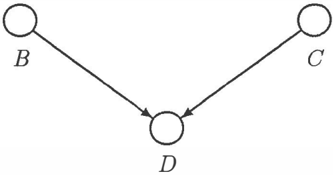
Figure 2: A more complex network
<details>
<summary>Image 2 Details</summary>
### Visual Description
## Diagram: Directed Node Connections
### Overview
The image depicts a simple directed graph with three nodes labeled **B**, **C**, and **D**. Arrows indicate unidirectional relationships: one from **B** to **D** and another from **C** to **D**. No additional labels, legends, or numerical data are present.
### Components/Axes
- **Nodes**:
- **B**: Positioned at the top-left.
- **C**: Positioned at the top-right.
- **D**: Positioned at the bottom-center.
- **Edges**:
- **B → D**: Arrow originates at **B** and terminates at **D**.
- **C → D**: Arrow originates at **C** and terminates at **D**.
- **No legends, axis titles, or scales** are visible.
### Detailed Analysis
- **Node Placement**:
- **B** and **C** are spatially equidistant from the center, flanking **D** symmetrically.
- **D** acts as a central convergence point for both **B** and **C**.
- **Edge Directionality**:
- All edges are unidirectional, with no bidirectional or self-looping connections.
- No edge labels or weights are provided.
### Key Observations
1. **Centralized Dependency**: **D** receives input from both **B** and **C**, suggesting a role as a sink or aggregator.
2. **Symmetry**: The layout is balanced, with **B** and **C** mirroring each other relative to **D**.
3. **Minimalism**: The diagram lacks annotations, colors, or contextual metadata beyond node labels.
### Interpretation
This diagram likely represents a simplified workflow, dependency graph, or process flow where **B** and **C** contribute to or influence **D**. The absence of additional context (e.g., edge labels, node attributes) limits granular interpretation. However, the directional arrows emphasize causality or sequential relationships: **B** and **C** precede **D** in the depicted process.
**Notable Patterns**:
- **D** is the sole recipient of input, indicating potential bottlenecks or centralization risks if scaled.
- The lack of outgoing edges from **D** suggests it may be a terminal node or require external processing beyond the diagram’s scope.
**Underlying Implications**:
- The structure could model systems where two independent sources (B/C) converge on a single target (D), such as data pipelines, decision trees, or resource allocation models.
- Further analysis would require additional metadata (e.g., edge weights, node capacities) to quantify relationships.
</details>
We now extend these results to enable us to cope with networks in which nodes may have more than one par ent. To do this we consider the qualitative effect of two converging links such as those in Figure 2. Since we are only dealing with singly connected networks, B and C are independent and the overall effect at D is determined by:
There are two ways of tackling the network of Figure 2 in probability theory. We can either base our calcula tion on probabilities of the form p(d I b) which implies the simplifying assumption that the effect of B on D is independent of the effect of C (and vice versa), or we can use the proper joint probabilities of the three events B, C, and D, using values of the form p( d I b, c).
$$\begin{array}{c}
\left[ \Delta v _ { a } ( d ) \right] = \left[ \frac{\partial u _ { a } ( b )}{\partial v _ { a } ( c )}\right] \cdot \left[ \frac{\partial u _ { a } ( c )}{\partial v _ { a } ( c )}\right] \cdot \left[ \frac{\partial u _ { a } ( c )}{\partial v _ { a } ( c )}\right]
\end{array}
\begin{array}{c}
\left[ \Delta v _ { b } ( d ) \right] = \left[ \frac{\partial u _ { b } ( c )}{\partial v _ { b } ( c )}\right] \cdot \left[ \frac{\partial u _ { b } ( c )}{\partial v _ { b } ( c )}\right] \cdot \left[ \frac{\partial u _ { b } ( c )}{\partial v _ { b } ( c )}\right]
\end{array}
\begin{array}{c}
\left[ \Delta v _ { c } ( d ) \right] = \left[ \frac{\partial u _ { c } ( c )}{\partial v _ { c } ( c )}\right] \cdot \left[ \frac{\partial u _ { c } ( c )}{\partial v _ { c } ( c )}\right] \cdot \left[ \frac{\partial u _ { c } ( c )}{\partial v _ { c } ( c )}\right]
\end{array}$$
In the first case we assume that the effects of B and C on D are completely independent of one another so that the variation of D with B (and D with C) is just as described by Theorem 3.1, the joint effect being established by using ( 4) to obtain:
which gives the same results as the expression given by Wellman [1990a] for evaluating the same situa tion. vVith the other approach, writing the network as B&C .... D, we have:
$$established by using (4) to obtain:$$
Theorem 5.1: The relation between p(z) and p(x) for the link B&C .... D is determined by:
$$\left[ \frac { \partial p ( z ) } { \partial p ( x ) } \right] = [ p ( z | x , y ) + p ( z - w , y )$$
$$- p ( z | x , y ) - p ( z | - w , y )$$
for all x E {b, -,b}, y{c, -,c} and z E {d, -,d}.
Proof: We have p(d) = LbE{b,-,b}cE{c,-,c} p(b, c, d) = Lbe{b,-,b}cE{c,..,c} p(b, c)p(d I b, c). Since B and C are independent, p(b, c) = p(b)p(c). Using p(x) = 1 p(-,x) and differentiating we find that [ 8p(d)\8p(b)] = p(c) [ p(d I b, c)-p(d I -,b, c)] + p( -, c) [p(d I b, -, c) - p(d I -,b,-,c)] = p(c){[p(d I b,c) + p(d I -,b,-,c)] - [(p(d I b, -, c) + p(d I -,b, c) ]} + [ (p(d I b, -,c)- p(d I ..,b, -,c) ] . From this, and similar results for the variation of p( d) with p(-,b), p(c) and p(-,c), and the way p(-,d) changes with p( b), p( -,b), p( c) and p( -,c), the result follows. D
Thus the way in which for instance p( d) is dependent upon p(b) is itself dependent upon a term just like the synergy condition introduced by Wellman, and apply ing ( 4) we get an expression which has a similar be haviour to that given by Wellman for a synergetic re lation. In possibility theory we have a similar result to that for the simple link:
Theorem 5.2: The relation between II(x), IT(y) and II(z), for all x E {b,-,b}, y E {c,..,c}, z E {d,-,d} for the link B&C .... D is such that:
- (1) II(z) follows II( x) iff II( x, y, z) > sup[II( ..,x, y, z), II(x,-.y,z),II(..,x,-,y,z)] and II(x) < min(II(z I x,y), II(y)), or II(x, -,y, z) > sup[II(x, y, z), II(..,x, y, z), II(-,x,..,y,z)] and II(x) < min(II(z I x,-,y),II(-,y)).
- (2) II(z) may follow II(x) up iff II(x, y, z) ::::; sup [ IT(-.x,y,z),IT(x,-.y,z),II(..,x,..,y,z)] and II(x) < min(II(z I x, y), II(y)), or II(x, -.y, z) ::::; sup[II(x, y, z), II( -,x, y, z), II(-,x, -,y, z) ] and II(x) < min(II(z I x, ..,y), II(-,y)).
- (3) II(z) may follow II(x) down iff II(x, y, z) > sup[II(-.x, y, z),II(x, -,y, z), II(-,x,-,y, z)] and II(x);::: min(IT(z I x, y), II(y)), or II(x, -,y, z) > sup[IT(x, y, z), II( -,x, y, z), II(-,x, -,y, z) ] and II(x) 2': min(IT(z I x,-,y),II(-,y)).
- (4) Otherwise II(z) is independent of II(x).
Proof: As for Theorem 3.2, the result may be de termined directly from IT(d) = SUPxe{x,..,x},YE{y,-,y} II(x,y,z) and II(x,y,z) = II(z I x,y)IT(x)II(y).D
When we use belief values we may take the relationship between B, C and D to be determined by one set of conditional beliefs of the form bel(d \ b, c), or by two sets of conditional beliefs of the form bel( dlb). For conditionals of the form bel(d I b, c) we have:
Theorem 5.3: The relation between bel(z) and bel(x) for the link B &C .... D is determined by:
$$\begin{aligned}
\{ \frac { | b ( z ) | } { | b ( x ) | } \} & = [ b ( z | x , y ) - b ( z | x - u , y ) ] \\
& = [ b ( z | x , - y ) - b ( z | x - u , - y ) ]
\end{aligned}$$
$$\begin{aligned}
& \textcircled { 1 } [ b ( z | x , y U - y ) ] - \textcircled { 2 } [ b ( z | x U - x , y U - y ) ] \\
& = \textcircled { 3 } [ b ( z | x U - x , y U - y ) ] + \textcircled { 4 } [ b ( z | x U - x , y U - y ) ]
\end{aligned}$$
For all x E {b,--,b}, y E {c,--,c}, z E {d,--,d}. Proof: By Dempster's rule of combination, bel(d) = Lb�{b,-.b},c�{c,-.c} m(b)m(c)bel(dib,c). Now, m(x) = bel(x), m(--,x) = bel(--,x) and m(x U --,x) = 1 -bel(x) -bel(--,x), so that [8bel(d)\8bel(b)] = [(bel(d I b, c) bel( d I b U --,b, c)] Ef) [(bel( d I b, -,c)-bel( d I b U --,b, -,c)] EB [ (bel(d I b, cu--,c)-bel(d I bu--,b, cu--,c). From this, and similar results for the variation of bel( d) with bel(--,b), bel(c) and bel(--,c), and the way bel(--,d) changes with bel(b), bel( --,b), bel( c) and bel( --,c) the result follows. D
Thus bel( d) follows bel(b) iff bel(d I b, c) > bel(d I bu--,b,c), bel(d I b,--,c) > bel(d I bu--,b,--,c), and bel(d I b, c U -,c) > bel(d I b U --,b, c U -,c). For conditionals of the form bel( d I b) we obtain:
Theorem 5.4: For the link B&C--+ D, bel(z) follows bel(x) if bel(z I x) � bel(zixU--,x) and is indeterminate otherwise for all x E {b,--,b}, y E {c,--,c}, z E {d,--,d}.
Proof : Dempster's rule of combination tells us that bel(d) = Lb�{b,-.b},c�{ c,-.c},bvc:Jd bel(dib)m(b) bel( dic)m( c). As a result, [8bel( d)\8bel(b )] = [(bel( d I b)-bel( d I bu--,b )]{bel( di--,c) [ 1 +bel( c )+bel( --,c) -m( c)] +bel( di--,c) [ 1 +bel( c)+ bel( -,c)-m( -,c)] +bel( die) [ 1 + bel(c) + bel(--,c)- m(c U -,c)]}+ bel(dl--,b) [m(c)bel(d I c)+ m(--,c)bel(d I -,c)+ m(c U --,c)bel(dic U -,c)). Since m(x) :::; 1 for all x, [8bel(d)\8bel(b)] = [+] if bel(d I b) � bel(dlb U -,b) and [?) otherwise. From this, and similar results for the variation of bel( d) with bel(--,b), bel(c) and bel(--,c), and the way bel(--,d) changes with bel(b), bel(--,b), bel(c) and bel(--,c) the result follows. D
Thus the formalisms again exhibit differences in be haviour across the same network.
The expressions derived in this section are those ob tained by using the precise theory of each formalism. This is important since it ensures the correctness of the integration introduced in Section 6. However, for reasoning using single formalisms, it may provde ad vantageous to extend the simpler apporach adopted by Wellman [1990a) to possibility and evidence theories.
Finally a word on the scope of the reasoning that we can perform as a result of our analysis. The differential calculus tells us that .6-z = Ax· [8z\8x] + .6-y · [8z\8y], provided that x is not a function of y. Thus we can clearly use the results derived above to propagate qual itative changes in probability, possibility and belief functions through any singly connected network.
## 6 INTEGRATION THROUGH QUALITATIVE CHANGE
The work described in this paper so far has extended qualitative reasoning about uncertainty handling for malisms to cover possibility and belief values as well as probability values. Not only is this useful in it self in providing a means of reasoning according to the precise rules of probability, possibility and Dempster Shafer theory when there is incomplete numerical in formation, but it can also provide a way of integrating the different formalisms.
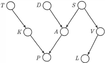
Consider the following medical example. The network of Figure 3 encodes the medical information that joint trauma (T) leads to loose knee bodies (K), and that these and arthritis (A) cause pain (P). The incidence of arthritis is influenced by dislocation (D) of the joint in question and by the patient suffering from Sjorgen 's syndrome (S) . Sjorgen's syndrome affects the inci dence of vasculitis (V), and vasculitis leads to vas culitic lesions (L).
<details>
<summary>Image 3 Details</summary>
### Visual Description
## Flowchart Diagram: Node-Based Process Flow
### Overview
The image depicts a directed graph with eight nodes labeled T, K, P, A, D, S, V, and L. Arrows indicate directional relationships between nodes, forming a hierarchical and interconnected structure. No numerical data, scales, or legends are present.
### Components/Axes
- **Nodes**:
- T, K, P, A, D, S, V, L (all uppercase letters).
- **Edges**:
- Directed arrows connecting nodes (e.g., T → K, K → P, P → A, A → D, A → S, S → V, V → L).
- **Structure**:
- Central node **A** acts as a hub, connecting to **D**, **S**, and **P**.
- **P** connects to **K**, which connects to **T**.
- **S** connects to **V**, which connects to **L**.
- No cycles; all paths terminate at leaf nodes (T, D, L).
### Detailed Analysis
- **Node Connections**:
- T → K → P → A (left branch).
- A → D (direct connection).
- A → S → V → L (right branch).
- **Flow Direction**:
- All edges point downward or to the right, suggesting a top-down or left-to-right workflow.
- **Missing Elements**:
- No labels for edges, no numerical values, no color coding, and no explicit legend.
### Key Observations
- **Central Hub**: Node **A** is the most connected, serving as a convergence point for multiple paths.
- **Termination Points**: Nodes T, D, and L are endpoints with no outgoing edges.
- **Symmetry**: The left (T-K-P-A) and right (A-S-V-L) branches mirror each other in structure but differ in node labels.
### Interpretation
This diagram likely represents a process flow, decision tree, or organizational hierarchy. The central node **A** could symbolize a critical decision point or resource, with paths diverging to different outcomes (e.g., T, D, L). The absence of numerical data or labels suggests the focus is on relationships rather than quantitative metrics. The hierarchical design implies a structured workflow where each node represents a step or entity dependent on its predecessors.
</details>
Figure 3: A network representing medical knowledge The strengths of these influences are given as proba bilities:
| p(k I p(k I p(a I p(a I | p(v Is) | | 0.1 | | | |
|---------------------------|-----------|----------|---------|-----|-------------|-----|
| | | t) --,t) | 0.6 0.2 | p(v | I--,s) | 0.3 |
| | d,s) | | 0.9 | p(a | 1--,d,s) | 0.6 |
| | d,--,s) | | 0.6 | p(a | I--,d,--,s) | 0.4 |
beliefs:
k, bel(p I
a)
bel(p I
k,--,a)
--,k, bel(p I
a)
k
bel(p I
U
--,k, k,
bel(p I
a)
a U
-,a)
--,k,
--,p I
-,a)
--,k, bel (
bel(
--,p I
0.9
0.7
0.7
0.6
0.7
0.5
=
=
=
=
a U
-,a)
0.4
All other conditional beliefs are zero and possibilities:
$$\begin{cases} \pi ( 1 - v ) = 1 \\ \pi ( - l | v ) = 0 . 1 \end{cases}$$
We can integrate this information allowing us to say how our belief in the patient in question being in pain,
and the possibility that the patient has vasculitic le sions, vary when we have new evidence that she is suffering from Sjorgen's syndrome. From the new ev idence we have �p(s) = [+], �p(-.s) = [-] , �p(t) = [0], �p( -.t) = [0], �p( d) = [0] and �p( -.d) = [0]. Since a change of [0] can never become a change of [ +] or [ -] we can ignore the latter changes. Now, from Theorem 3.1 and Theorem 5. 1 we know that:
$$\left[ \frac { \partial p ( v ) } { \partial p ( s ) } \right] = - 1 \quad \text{and} \quad \left[ \frac { \partial p ( v ) } { \partial p ( - s ) } \right] = + 1$$
so that �p(a) =[+], and �p(v) =[-] from which we can deduce that �p(-.a) =[-] and �p(-.v) = [+].
To continue our reasoning we need to establish the change in belief of a and the change in possibility of l. To do this we make the monotonicity assumption [Parsons 1993] that if the probability of a hypothesis increases then both the possibility of that hypothesis and the belief in it do not decrease. As well as being intuitively acceptable, this assumption is the weakest sensible relation between values expressed in different formalisms, and is compatible both with the principle of consistency between probability and possibility val ues laid down by Zadeh [1978] and the natural exten sion of this principle to belief, necessity [Dubois and Prade 1988b], and plausibility values.
The assumption also says that if the probability de creases then the possibility and belief do not increase, and so we can say that �bel( a)= [+, OJ, �bel(-.a) = [ - , 0], �II(v) = [ -,0] and �II(-.v) = [+, 0]. Now we apply Theorem 5.3 to find that:
$$\begin{array}{ll}
\left[ \frac{\partial b e l ( p )}{\partial b e l ( a ) } \right] = [ + ] \\
\left[ \frac{\partial b e l ( - p )}{\partial b e l ( a ) } \right] = [ - ]
\end{array}$$
Since we are initially ignorant about the possibility of vasculitis, we have II(v) = II(-.v) = 1, so that Theo rem 3.2 gives:
$$\begin{aligned}
\left[ \frac { \partial p ( t ) } { \partial p ( v ) } \right] = [ 0 ] \\
\left[ \frac { \partial p ( - t ) } { \partial p ( - v ) } \right] = [ 0 ]
\end{aligned}$$
Hence we can tell that �bel(p) = [+, 0], bel(-.p) [ -, OJ and �II( v) = �II( -.v) = [OJ. The result of the new evidence is that belief in the patient's pain may in crease, while the possibility of the patient having vas culitic lesions is unaffected. Thus we can use numeri cal values and qualitative relationships from different uncertainty handling formalisms to reason about the change in the belief of some event given information about the probability of a second event, and can in fer whether the possibility of a third event also varies. As a result reasoning about qualitative change allows some integration between formalisms.
## 7 DISCUSSION
There is an important difference between the approach to qualitative reasoning under uncertainty described here, and that of Wellman [1990a, bJ. Despite their name, Wellman's Qualitative Probabilistic Networks do not describe the qualitative behaviour of probabilis tic networks exactly. In particular, some dependencies between variables are ignored in favour of simplicity, and synergy relations are sometimes introduced to rep resent them where it is considered to be important.
In our approach, since it is based directly upon the various formalisms, the qualitative changes predicted are exactly those of the quantitative methods. This has been demonstrated in [Parsons and Saffiotti 1993J which analyses the representation of a real problem in a number of different qualitative and quantitative for malisms. In this analysis we make qualitative predic tions about the impact of evidence of faults in an elec tricity distribution network and compare these with the real quantitative changes. In every ca<;e, for proba bility, possibility and belief values, the qualitative pre dictions were correct. This verification is a good in dication of the validity of the approach, and suggests that it will be useful in situations where incomplete information prevents the application of quantitative methods.
Our qualitative method also provides a means of in tegrating uncertainty handling formalisms on a purely syntactic basis. For any hypothesis x about which we have uncertain information expressed, say in proba bility theory and possibility theory, we can make the intuitively reasonable assumption that if p( x ) increases II( x ) does not decrease, and thus translate from proba bility to possibility without worrying what probability or possibility actually mean.
As a result any desired semantics may be attached to the values, a feature which finesses the problem of the acceptability of the semantics which must be faced by other, semantically based, schemes for integration (eg. [Baldwin 1991]). The only problem with switch ing semantics would be that some combination rules might no longer apply, Dempster's rule in the case of Baldwin's voting model semantics, which would entail a re-derivation of the appropriate propagation condi tions. Since the qualitative approach does not a priori, rule out any combination scheme, this is not a major difficulty.
Finally, there is one important way that this method might be improved. The main disadvantage of any qualitative system is that there is no distinction be tween small values and large values, so 0.001 is qualita tively the same as 100, 000. As a result we cannot dis tinguish between evidence that induces small changes in the certainty of a hypothesis and evidence that in duces large changes. This problem has been recognised for some time, and there is now a large body of work on order of magnitude reasoning (for example [Raiman
1986], [Parsons and Dohnal 1992]) which attempts to automate reasoning of the form it "If A is bigger than B and B is bigger than C then A is bigger than C". The applications to our system are obvious, and we intend to do some work on this in the near future.
## 8 SUMMARY
This paper has introduced a new method for qualita tive reasoning under uncertainty which is equally ap plicable to all uncertainty handling techniques. All that need be done to find the qualitative relation be tween two values is to write down the analytical ex pression relating them and take the derivative of this expression with respect to one of the values. This fact was illustrated by results from the qualitative analysis of the simplest possible reasoning networks in each of the three most widely used formalisms.
Having established the qualitative behaviours of prob ability, possibility and evidence theories, the differ ences between these behaviours were discussed at some length, before knowledge of this behaviour was used to establish a form of qualitative integration between for malisms. In this integration numerical and qualitative data expressed in all three formalisms was used to help derive the change in belief of one node in a directed graph and the possibility of another from knowledge of a change in the probability of a third, related, node.
## Acknowledgements
The work of the first author was partially supported by a grant from ESPRIT Basic Research Action 3085 DRUMS, and he is endebted to all of his colleagues on the project for their help and advice.
Special thanks are due to Mirko Dohnal, Didier Dubois, John Fox, Frank Klawonn, Paul Krause, Rudolf Kruse, Henri Prade, Alessandro Saffiotti and Philippe Smets for uncomplaining help and construc tive criticism. The anonymous referees also made a number of useful comments.
## References
Baldwin, J. F. (1991) The Management of Fuzzy and Probabilistic Uncertainties for Knowledge Based Sys tems, in Encyclopaedia of Artificial Intelligence (2nd Edition), John Wiley & Sons, New York.
Dubois, D. and Prade, H. (1991) Conditional objects and non-monotonic reasoning, Proceedings of the 2nd International Conference on Principles of Knowledge Representation and Reasoning, Morgan Kaufmann. Cambridge, MA.
Dubois, D. and Prade, H. (1988a) Possibility Theory: An Approach to Computerised Processing of Uncer tainty, Plenum Press, New York.
Dubois, D. and Prade, H. (1988b) Modelling uncer- tainty and inductive inference: a survey of recent non additive probability systems, Acta Psychologica, 68, pp 53-78.
Farreny, H. and Prade, H. (1989) Positive and negative explanations of uncertain reasoning in the framework of possibility theory, Proceedings of the 5th Workshop on Uncertainty in Artificial Intelligence, Windsor.
Fonck, P. and Straszecka, E. (1991) Building influence networks in the framework of possibility theory, An nates Univ. Sci. Budapest., Sect. Camp. 12, pp 101 106.
Henrion, M. and Druzdzel, M. J. (1990) Qualitative propagation and scenario-based approaches to expla nation of probabilistic reasoning, Proceedings of the 6th Conference on Uncertainty in AI, Boston.
Parsons, S. (1993) Qualitative methods for reasoning under uncertainty, PhD Thesis, Department of Elec tronic Engineering, Queen Mary and Westfield Col lege. (in preparation).
Parsons, S. (1992a) Qualitative possibilistic networks. Proceedings of the International Conference on Infor mation Processing and Management of Uncertainty, Palma de Mallorca.
Parsons, S. (1992b) Qualitative belief networks. Pro ceedings of the 1Oth European Conference on Artificial Intelligence, Vienna.
Parsons, S. and Dohnal, M. (1993) A semiqualitative approach to reasoning in probabilistic networks, Ap plied Artificial Intelligence, 7, pp 223-235.
Parsons, S. and Saffiotti, A. (1993) A case study in the qualitative verification and debugging of quantita tive uncertainty, Technical Report, IRIDIA/TR/93-1, Universite Libre de Bruxelles.
Pearl, J. (1988) Probabilistic reasoning in intelli gent systems: networks of plausible inference, Morgan Kaufman, San Mateo, CA.
Raiman, 0. (1986) Order of magnitude reasoning, Pro ceedings of the 5th National Conference on Artificial Intelligence, Philadelphia.
Shafer, G. (1976) A mathematical theory of evidence, Princeton University Press, Princeton, NJ.
Smets, Ph. (1991) Belief functions: the disjunctive rule of combination and the generalized bayesian the orem, Technical Report TR/IRIDIA/91-01-2, Univer site Libre de Bruxelles.
Wellman, M.P. (1990a) Fundamental concepts of qual itative probabilistic networks, Artificial Intelligence, 44, pp 257-303.
Wellman, M. P. (1990b) Formulation of tradeoffs in planning under uncertainty, Pitman, London.
Zadeh, L. A. (1978) Fuzzy sets as a basis for a theory of possibility, Fuzzy Sets and Systems, 1, pp 1-28.