# Unknown Title
## Graphic lambda calculus
Marius Buliga
Institute of Mathematics, Romanian Academy P.O. BOX 1-764, RO 014700 Bucure¸ sti, Romania
Marius.Buliga@imar.ro
This version: 23.05.2013
## Abstract
We introduce and study graphic lambda calculus, a visual language which can be used for representing untyped lambda calculus, but it can also be used for computations in emergent algebras or for representing Reidemeister moves of locally planar tangle diagrams.
## 1 Introduction
Graphic lambda calculus consists of a class of graphs endowed with moves between them. It might be considered a visual language in the sense of Erwig [9]. The name 'graphic lambda calculus' comes from the fact that it can be used for representing terms and reductions from untyped lambda calculus. It's main move is called 'graphic beta move' for it's relation to the beta reduction in lambda calculus. However, the graphic beta move can be applied outside the 'sector' of untyped lambda calculus, and the graphic lambda calculus can be used for other purposes than the one of visual representing lambda calculus.
For other visual, diagrammatic representation of lambda calculus see the VEX language [8], or David Keenan's [15].
The motivation for introducing graphic lambda calculus comes from the study of emergent algebras. In fact, my goal is to build eventually a logic system which can be used for the formalization of certain 'computations' in emergent algebras, which can be applied then for a discrete differential calculus which exists for metric spaces with dilations, comprising riemannian manifolds and sub-riemannian spaces with very low regularity.
Emergent algebras are a generalization of quandles, namely an emergent algebra is a family of idempotent right quasigroups indexed by the elements of an abelian group, while quandles are self-distributive idempotent right quasigroups. Tangle diagrams decorated by quandles or racks are a well known tool in knot theory [10] [13].
It is notable to mention the work of Kauffman [14], where the author uses knot diagrams for representing combinatory logic, thus untyped lambda calculus. Also Meredith and Snyder[17] associate to any knot diagram a process in pi-calculus,
Is there any common ground between these three apparently separated field, namely differential calculus, logic and tangle diagrams? As a first attempt for understanding this, I proposed λ -Scale calculus [5], which is a formalism which contains both untyped lambda calculus and emergent algebras. Also, in the paper [6] I proposed a formalism of decorated tangle diagrams for emergent algebras and I called 'computing with space' the various manipulations of these diagrams with geometric content. Nevertheless, in that paper I was not able to give a precise sense of the use of the word 'computing'. I speculated, by using analogies from studies of the visual system, especially the 'Brain a geometry engine' paradigm of Koenderink [16], that, in order for the visual front end of the brain to reconstruct the visual space in the brain, there should be a kind of 'geometrical computation' in the
neural network of the brain akin to the manipulation of decorated tangle diagrams described in our paper.
I hope to convince the reader that graphic lambda calculus gives a rigorous answer to this question, being a formalism which contains, in a sense, lambda calculus, emergent algebras and tangle diagrams formalisms.
Acknowledgement. This work was supported by a grant of the Romanian National Authority for Scientific Research, CNCS UEFISCDI, project number PN-II-ID-PCE-2011-30383.
## 2 Graphs and moves
An oriented graph is a pair ( V, E ), with V the set of nodes and E ⊂ V × V the set of edges. Let us denote by α : V → 2 E the map which associates to any node N ∈ V the set of adjacent edges α ( N ). In this paper we work with locally planar graphs with decorated nodes, i.e. we shall attach to a graph ( V, E ) supplementary information:
- -a function f : V → A which associates to any node N ∈ V an element of the 'graphical alphabet' A (see definition 2.1),
- -a cyclic order of α ( N ) for any N ∈ V , which is equivalent to giving a local embedding of the node N and edges adjacent to it into the plane.
We shall construct a set of locally planar graphs with decorated nodes, starting from a graphical alphabet of elementary graphs. On the set of graphs we shall define local transformations, or moves. Global moves or conditions will be then introduced.
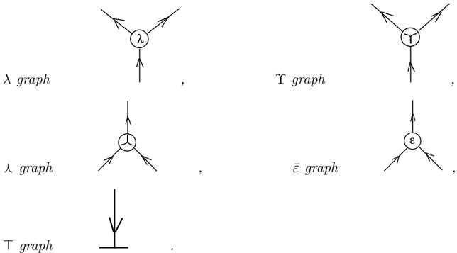
Definition 2.1 The graphical alphabet contains the elementary graphs, or gates, denoted by λ , Υ , , , and for any element ε of the commutative group Γ , a graph denoted by ¯ ε . Here are the elements of the graphical alphabet:
<details>
<summary>Image 1 Details</summary>
### Visual Description
## Diagram: Symbolic Graph Structures
### Overview
The image depicts five labeled graph structures arranged in two columns. Each graph uses directional arrows and central symbols to represent relationships or processes. The graphs are labeled with Greek letters (λ, λ, T, Υ, ε) and described as "graphs" (e.g., "λ graph," "Υ graph").
### Components/Axes
- **Left Column**:
1. **λ graph**: Three arrows radiating outward from a central circle labeled "λ."
2. **λ graph**: Three arrows radiating outward from a central circle labeled "λ," with a smaller circle inside the main circle.
3. **T graph**: A single vertical arrow pointing downward from a horizontal line (resembling a "T" shape).
- **Right Column**:
4. **Υ graph**: Three arrows radiating outward from a central circle labeled "Υ."
5. **ε graph**: Three arrows radiating outward from a central circle labeled "ε."
### Detailed Analysis
- **λ graphs**: Both instances show three outward-pointing arrows, suggesting a branching or distributive process. The second λ graph includes a nested circle, possibly indicating a sub-component or hierarchical relationship.
- **T graph**: The vertical arrow implies a unidirectional flow or termination point, distinct from the branching structures.
- **Υ and ε graphs**: Similar to the λ graphs but with unique central symbols (Υ and ε), potentially denoting specialized operations or states.
### Key Observations
- The repetition of the λ graph with slight variations (nested circle) suggests iterative or layered processes.
- The T graph’s simplicity contrasts with the complexity of the other graphs, possibly representing a base case or endpoint.
- The Υ and ε graphs introduce new symbols, which may signify distinct categories or transformations.
### Interpretation
This diagram likely represents abstract computational or logical processes, where:
- **λ graphs** model branching operations (e.g., function application, data distribution).
- The **T graph** could symbolize a terminal state or linear progression.
- **Υ and ε graphs** might represent specialized operations (e.g., unification, error handling) given their unique symbols.
- The nested circle in the second λ graph hints at recursion or nested dependencies.
The arrangement in two columns may categorize graphs by type (e.g., branching vs. specialized operations). No numerical data is present, so trends or quantitative analysis cannot be derived. The focus is on structural relationships and symbolic meaning.
</details>
With the exception of the , all other elementary graphs have three edges. The graph has only one edge.
There are two types of 'fork' graphs, the λ graph and the Υ graph, and two types of 'join' graphs, the graph and the ¯ ε graph. Further I briefly explain what are they supposed to represent and why they are needed in this graphic formalism.
The λ gate corresponds to the lambda abstraction operation from untyped lambda calculus. This gate has one input (the entry arrow) and two outputs (the exit arrows), therefore, at first view, it cannot be a graphical representation of an operation. In untyped lambda calculus the λ abstraction operation has two inputs, namely a variable name x and a term A , and one output, the term λx.A . There is an algorithm, presented in section 3, which
transforms a lambda calculus term into a graph made by elementary gates, such that to any lambda abstraction which appears in the term corresponds a λ gate.
The Υ gate corresponds to a FAN-OUT gate. It is needed because the graphic lambda calculus described in this article does not have variable names. Υgates appear in the process of elimination of variable names from lambda terms, in the algorithm previously mentioned.
Another justification for the existence of two fork graphs is that they are subjected to different moves: the λ gate appears in the graphic beta move, together with the gate, while the Υ gate appears in the FAN-OUT moves. Thus, the λ and Υ gates, even if they have the same topology, they are subjected to different moves, which in fact characterize their 'lambda abstraction'-ness and the 'fan-out'-ness of the respective gates. The alternative, which consists into using only one, generic, fork gate, leads to the identification, in a sense, of lambda abstraction with fan-out, which would be confusing.
The gate corresponds to the application operation from lambda calculus. The algorithm from section 3 associates a gate to any application operation used in a lambda calculus term.
The ¯ ε gate corresponds to an idempotent right quasigroup operation, which appears in emergent algebras, as an abstractization of the geometrical operation of taking a dilation (of coefficient ε ), based at a point and applied to another point.
As previously, the existence of two join gates, with the same topology, is justified by the fact that they appear in different moves.
1. The set GRAPH. We construct the set of graphs GRAPH over the graphical alphabet by grafting edges of a finite number of copies of the elements of the graphical alphabet.
Definition 2.2 GRAPH is the set of graphs obtained by grafting edges of a finite number of copies of the elements of the graphical alphabet. During the grafting procedure, we start from a set of gates and we add, one by one, a finite number of gates, such that, at any step, any edge of any elementary graph is grafted on any other free edge (i.e. not already grafted to other edge) of the graph, with the condition that they have the same orientation.
For any node of the graph, the local embedding into the plane is given by the element of the graphical alphabet which decorates it.
The set of free edges of a graph G ∈ GRAPH is named the set of leaves L ( G ) . Technically, one may imagine that we complete the graph G ∈ GRAPH by adding to the free extremity of any free edge a decorated node, called 'leaf', with decoration 'IN' or 'OUT', depending on the orientation of the respective free edge. The set of leaves L ( G ) thus decomposes into a disjoint union L ( G ) = IN ( G ) ∪ OUT ( G ) of in or out leaves.
Moreover, we admit into GRAPH arrows without nodes, , called wires or lines, and loops (without nodes from the elementary graphs, nor leaves)
<details>
<summary>Image 2 Details</summary>
### Visual Description
## Diagram: Simple Cyclic Process
### Overview
The image depicts a minimalist diagram of a continuous loop with an arrow indicating directionality. No textual labels, legends, or numerical data are present. The loop is irregularly shaped, resembling an oval or ellipse, with a single arrowhead positioned on the right side of the loop.
### Components/Axes
- **Loop**: A closed, irregularly shaped oval occupying the central area of the image.
- **Arrow**: A single arrowhead located on the right side of the loop, pointing counterclockwise (toward the top-left of the loop).
- **Background**: Plain white, with no additional elements or annotations.
### Detailed Analysis
- The loop’s irregular shape suggests a non-uniform or dynamic process.
- The arrow’s placement and direction imply a cyclical flow, starting from the right side and moving counterclockwise around the loop.
- No numerical values, categories, or sub-categories are present.
### Key Observations
- The absence of text or labels leaves the specific nature of the process ambiguous.
- The counterclockwise arrow could symbolize repetition, feedback, or a recurring cycle.
- The simplicity of the diagram emphasizes the concept of continuity rather than discrete steps.
### Interpretation
This diagram likely represents a conceptual model of a continuous process, such as a feedback loop, iterative workflow, or recurring event. The counterclockwise arrow reinforces the idea of cyclicality, while the lack of additional details suggests the focus is on the loop’s persistence rather than its components. The irregular shape of the loop may imply variability or adaptability within the cycle.
**Note**: No factual or numerical data is extractable from the image. The description is based solely on visual elements.
</details>
Graphs in GRAPH can be disconnected. Any graph which is a finite reunion of lines, loops and assemblies of the elementary graphs is in GRAPH .
2. Local moves. These are transformations of graphs in GRAPH which are local, in the sense that any of the moves apply to a limited part of a graph, keeping the rest of the graph unchanged.
We may define a local move as a rule of transformation of a graph into another of the following form.
First, a subgraph of a graph G in GRAPH is any collection of nodes and/or edges of G . It is not supposed that the mentioned subgraph must be in GRAPH . Also, a collection
of some edges of G , without any node, count as a subgraph of G . Thus, a subgraph of G might be imagined as a subset of the reunion of nodes and edges of G .
For any natural number N and any graph G in GRAPH , let P ( G,N ) be the collection of subgraphs P of the graph G which have the sum of the number of edges and nodes less than or equal to N .
Definition 2.3 A local move has the following form: there is a number N and a condition C which is formulated in terms of graphs which have the sum of the number of edges and nodes less than or equal to N , such that for any graph G in GRAPH and for any P ∈ P ( G,N ) , if C is true for P then transform P into P ′ , where P ′ is also a graph which have the sum of the number of edges and nodes less than or equal to N .
Graphically we may group the elements of the subgraph, subjected to the application of the local rule, into a region encircled with a dashed closed, simple curve. The edges which cross the curve (thus connecting the subgraph P with the rest of the graph) will be numbered clockwise. The transformation will affect only the part of the graph which is inside the dashed curve (inside meaning the bounded connected part of the plane which is bounded by the dashed curve) and, after the transformation is performed, the edges of the transformed graph will connect to the graph outside the dashed curve by respecting the numbering of the edges which cross the dashed line.
However, the grouping of the elements of the subgraph has no intrinsic meaning in graphic lambda calculus. It is just a visual help and it is not a part of the formalism. As a visual help, I shall use sometimes colors in the figures. The colors, as well, don't have any intrinsic meaning in the graphic lambda calculus.
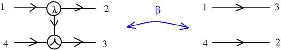
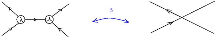
2.1. Graphic β move. This is the most important move, inspired by the β -reduction from lambda calculus, see theorem 3.1, part (d).
<details>
<summary>Image 3 Details</summary>
### Visual Description
## Diagram: Structural Relationship Between Two Directed Graphs
### Overview
The image depicts two directed graphs connected by a bidirectional arrow labeled β. The left graph contains nodes 1, 2, 3, 4 with internal transformations (λ and △ symbols), while the right graph shows a linear sequence 1→3→4→2. The bidirectional β arrow suggests a structural equivalence or transformation between the two graphs.
### Components/Axes
- **Left Graph**:
- Nodes: 1, 2, 3, 4 (labeled sequentially)
- Transformations:
- Node 1 → Node 2 (horizontal arrow)
- Node 4 → Node 3 (horizontal arrow)
- Vertical connection between Node 2 and Node 3 via:
- Circle with λ symbol (top)
- Circle with △ symbol (bottom)
- **Right Graph**:
- Linear path: 1 → 3 → 4 → 2 (all horizontal arrows)
- **Connecting Element**:
- Bidirectional arrow labeled β between the two graphs
### Detailed Analysis
1. **Left Graph Structure**:
- Two parallel horizontal flows:
- Top: 1 → 2 (λ symbol at midpoint)
- Bottom: 4 → 3 (△ symbol at midpoint)
- Vertical coupling between 2 and 3 via dual symbols (λ and △)
- Nodes 1 and 4 act as sources; nodes 2 and 3 as sinks
2. **Right Graph Structure**:
- Sequential flow: 1 → 3 → 4 → 2
- No internal transformations (pure linear path)
- Node 3 serves as an intermediate hub
3. **β Relationship**:
- Bidirectional connection implies:
- Possible isomorphism between graph structures
- Transformation mapping between equivalent nodes
- Preservation of node identities (1→1, 2→2, 3→3, 4→4)
### Key Observations
- Node 3 appears in both graphs but with different roles:
- Left: Terminal node (sink)
- Right: Intermediate node
- The λ and △ symbols may represent:
- λ: Merge operation (converging paths)
- △: Split operation (diverging paths)
- β's bidirectional nature suggests reversible transformation
### Interpretation
This diagram likely represents:
1. **Graph Isomorphism**: The β arrow indicates the two graphs are structurally equivalent despite different node arrangements
2. **Process Transformation**: The λ/△ symbols in the left graph (parallel processing) transform into the linear sequence in the right graph through β
3. **Node Preservation**: All nodes maintain their identities across graphs, suggesting β is an identity-preserving mapping
4. **Topological Equivalence**: The presence of both parallel and sequential paths implies the system can operate in multiple configurations while maintaining core functionality
The diagram appears to model a computational or mathematical system where parallel processing (left) and sequential execution (right) are interconvertible through β, with node identities preserved across transformations.
</details>
The labels '1, 2, 3, 4' are used only as guides for gluing correctly the new pattern, after removing the old one. As with the encircling dashed curve, they have no intrinsic meaning in graphic lambda calculus.
This 'sewing braids' move will be used also in contexts outside of lambda calculus! It is the most powerful move in this graphic calculus. A primitive form of this move appears as the re-wiring move (W1) (section 3.3, p. 20 and the last paragraph and figure from section 3.4, p. 21 in [6]).
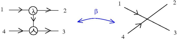
An alternative notation for this move is the following:
<details>
<summary>Image 4 Details</summary>
### Visual Description
## Diagram: Bidirectional Transformation Between Two Structures
### Overview
The image depicts a bidirectional relationship (labeled **β**) between two distinct diagrammatic structures. The left structure consists of a directed graph with labeled nodes and symbolic operations, while the right structure shows intersecting lines with numerical labels. The bidirectional arrow **β** suggests equivalence, transformation, or duality between the two systems.
---
### Components/Axes
1. **Left Diagram**:
- **Nodes**:
- Node **1** (top-left) → Node **2** (top-right) via a directed arrow.
- Node **4** (bottom-left) → Node **3** (bottom-right) via a directed arrow.
- **Symbols**:
- Node **1** contains the symbol **λ** (lambda).
- Node **4** contains a triangular symbol (△).
- **Flow**: Arrows indicate directional relationships (1→2, 4→3).
2. **Right Diagram**:
- **Lines**: Two intersecting lines labeled **1**, **2**, **3**, **4** (clockwise from top-left).
- **Arrows**: Bidirectional arrows on the intersecting lines, suggesting mutual interaction or transformation.
3. **Bidirectional Relationship**:
- **β**: A curved double-headed arrow connecting the left and right diagrams, labeled **β** (beta).
---
### Detailed Analysis
- **Left Diagram**:
- The symbols **λ** and **△** likely represent specific operations or transformations applied to nodes 1 and 4, respectively.
- The directed arrows (1→2, 4→3) imply a sequential or causal relationship between nodes.
- **Right Diagram**:
- The intersecting lines labeled **1–4** may represent a transformed or equivalent state of the left diagram’s nodes, with the crossing points indicating interactions or dependencies.
- **β Relationship**:
- The bidirectional arrow **β** implies a reversible or symmetric relationship between the two structures. This could denote:
- A mathematical equivalence (e.g., isomorphism).
- A process transformation (e.g., input-output mapping).
- A duality in system behavior.
---
### Key Observations
1. **Symbolic Operations**: The use of **λ** and **△** suggests specialized functions or rules governing the left diagram’s nodes.
2. **Structural Equivalence**: The right diagram’s intersecting lines mirror the left diagram’s node connections, hinting at a transformed or abstracted representation.
3. **Bidirectional Flow**: The **β** arrow emphasizes reciprocity, suggesting the relationship is not unidirectional.
---
### Interpretation
This diagram likely illustrates a conceptual or mathematical framework where:
- The left structure represents a **source system** with explicit operations (**λ**, **△**) and directional dependencies.
- The right structure represents a **transformed system** where interactions are abstracted into intersecting lines, possibly simplifying or generalizing the original relationships.
- The **β** relationship bridges these systems, indicating they are equivalent under certain conditions (e.g., a homomorphism, duality, or isomorphism).
The absence of numerical data or explicit units suggests this is a **conceptual diagram** rather than an empirical chart. The focus is on illustrating relationships, transformations, or equivalences between two abstract systems.
</details>
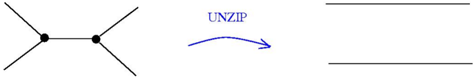
A move which looks very much alike the graphic beta move is the UNZIP operation from the formalism of knotted trivalent graphs, see for example the paper [21] section 3. In order to see this, let's draw again the graphic beta move, this time without labeling the arrows:
<details>
<summary>Image 5 Details</summary>
### Visual Description
## Diagram: Process Flow with Transformation Symbol (β)
### Overview
The image depicts two schematic diagrams connected by a bidirectional blue arrow labeled "β". The left diagram shows a node-based system with directional flows, while the right diagram represents a crossed structure with directional arrows. Both diagrams use standardized arrow notation for flow representation.
### Components/Axes
1. **Left Diagram**:
- **Node λ**: Circular node with three directional arrows (two incoming, one outgoing)
- **Node β**: Circular node with three outgoing arrows
- **Connection**: Single arrow from λ to β
- **Arrow Style**: Black lines with arrowheads
2. **Right Diagram**:
- **Crossed Structure**: Two intersecting black lines forming an "X"
- **Directional Arrows**: Four arrows (two on each line) pointing outward from the intersection
- **Label**: Blue bidirectional arrow labeled "β" above the crossed structure
3. **Shared Element**:
- **Transformation Symbol**: Blue bidirectional arrow labeled "β" connecting both diagrams
### Detailed Analysis
- **Left Diagram Flow**:
- Inputs converge on λ (two arrows)
- Single output from λ to β
- β distributes output to three paths
- Suggests a processing/transformation sequence: λ → β → multiple outputs
- **Right Diagram Structure**:
- Crossed lines with outward-pointing arrows
- Represents bidirectional interaction or opposition
- β label implies this structure is the result/manifestation of the β transformation
### Key Observations
1. β appears in both diagrams but serves different roles:
- Left: Transformation node
- Right: Resulting structure
2. Directional consistency:
- All arrows use standard arrowhead notation
- Bidirectional β arrow contrasts with unidirectional diagram flows
3. Symmetry:
- Left diagram has 3 input/output points
- Right diagram has 4 directional endpoints
### Interpretation
This appears to represent a system transformation process:
1. Initial state (λ) receives multiple inputs
2. Undergoes β transformation (possibly a catalytic or mediating process)
3. Produces β as an emergent structure (the crossed X)
4. The X structure then distributes energy/flow in four directions
The β symbol's bidirectional nature suggests reversible transformation, while the crossed X might represent:
- Opposition/conflict resolution
- Interlocking systems
- Phase transition point
- Equilibrium state
The diagram likely models a physical/chemical process (e.g., molecular interaction) or abstract system dynamics (e.g., decision-making flow). The precise nature requires domain-specific context.
</details>
The unzip operation acts only from left to right in the following figure. Remarkably, it acts on trivalent graphs (but not oriented).
<details>
<summary>Image 6 Details</summary>
### Visual Description
## Diagram: Molecular Unzipping Process
### Overview
The image depicts a molecular structure on the left, a labeled arrow ("UNZIP") pointing to the right, and an empty space on the far right. The diagram suggests a transformation or process from the initial molecular configuration to a final state.
### Components/Axes
- **Left Side**: A molecular structure with two central atoms (represented as black dots) connected by a single bond. Each central atom has three branches extending outward at 120° angles, forming a planar, symmetrical arrangement.
- **Center**: A blue dashed arrow labeled "UNZIP" in uppercase letters, pointing from the molecular structure to the right.
- **Right Side**: A blank rectangular space with no visible features, implying a transformed or "unzipped" state.
### Detailed Analysis
- **Molecular Structure**: The left-side molecule resembles a simplified representation of a linear or trigonal planar molecule (e.g., CO₂ or a substituted ethylene). The two central atoms are bonded, with three substituents per atom.
- **Arrow and Label**: The "UNZIP" label is positioned centrally above the arrow, which spans horizontally across the image. The arrow’s dashed line and direction imply a process of separation or bond cleavage.
- **Right Side**: The absence of features on the right suggests a linear or fully extended molecular conformation, consistent with the term "unzip."
### Key Observations
1. The "UNZIP" label explicitly indicates a bond-breaking or structural rearrangement process.
2. The molecular structure’s symmetry (three branches per atom) contrasts with the blank right side, emphasizing a transition from ordered to disordered or extended states.
3. No numerical data, scales, or legends are present, confirming this is a conceptual diagram rather than a quantitative chart.
### Interpretation
The diagram likely represents a chemical or physical process where a molecule undergoes bond cleavage or conformational change. The term "UNZIP" metaphorically describes the separation of bonded atoms or subunits, analogous to unzipping a zipper. The left-side molecule’s symmetry and the right-side blank space suggest a transition from a compact, ordered structure to a linear or fragmented state. This could model processes like polymer degradation, DNA strand separation, or molecular dissociation. The simplicity of the diagram prioritizes conceptual clarity over quantitative detail, focusing on the directional flow of the transformation.
</details>
Let us go back to the graphic beta move and remark that it does not depend on the particular embedding in the plane. For example, the intersection of the '1,3' arrow with the '4,2' arrow is an artifact of the embedding, there is no node there. Intersections of arrows have no meaning, remember that we work with graphs which are locally planar, not globally planar.
The graphic beta move goes into both directions. In order to apply the move, we may pick a pair of arrows and label them with '1,2,3,4', such that, according to the orientation of the arrows, '1' points to '3' and '4' points to '2', without any node or label between '1' and '3' and between '4' and '2' respectively. Then, by a graphic beta move, we may replace the portions of the two arrows which are between '1' and '3', respectively between '4' and '2', by the pattern from the LHS of the figure.
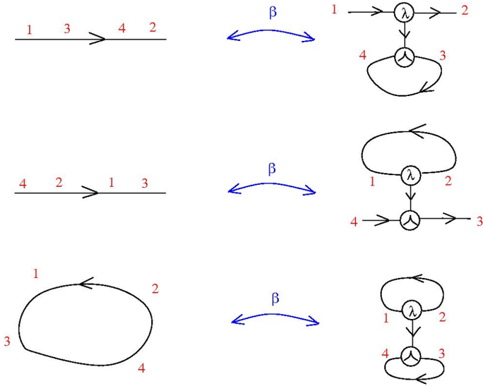
The graphic beta move may be applied even to a single arrow, or to a loop. In the next figure we see three applications of the graphic beta move. They illustrate the need for considering loops and wires as members of GRAPH .
<details>
<summary>Image 7 Details</summary>
### Visual Description
## Diagram: Linear-to-Network Transformation Flow
### Overview
The image presents a comparative analysis of three linear sequences (left) and their corresponding network representations (right), connected by bidirectional arrows labeled β. The diagrams use numbered nodes (1-4) and directional arrows to depict relationships, with β serving as a transformative or equivalence operator between linear and network structures.
### Components/Axes
- **Nodes**: Labeled 1, 2, 3, 4 (red text)
- **Arrows**:
- Linear flow (→) in left diagrams
- Bidirectional β arrows (↔️) between left/right sections
- Cyclic loops (→→) in specific nodes
- **Central Nodes**:
- λ (lambda) in right diagrams (black text)
- Y-shaped node in right diagrams (black text)
- **β Arrows**: Positioned centrally between left/right sections, suggesting transformation equivalence
### Detailed Analysis
#### Left Section (Linear Sequences)
1. **First Diagram**: 1 → 3 → 4 → 2 (linear progression)
2. **Second Diagram**: 4 → 2 → 1 → 3 (reversed order)
3. **Third Diagram**: 1 → 2 → 3 → 4 → 1 (cyclic loop)
#### Right Section (Network Structures)
1. **First Diagram**:
- Central λ node connected to 1 (↑) and 2 (→)
- Loop between 4 (↑) and 3 (→)
2. **Second Diagram**:
- λ node connected to 1 (↑) and 2 (→)
- 4 connected to 3 (→)
3. **Third Diagram**:
- λ node connected to 1 (↑) and 2 (→)
- 4 connected to 3 (→) with loop 3 → 4
### Key Observations
1. **Reversal Symmetry**: The second left diagram inverts the first, suggesting β may represent bidirectional transformation.
2. **Cyclic Processes**: Both left third and right first diagrams feature loops, indicating persistent states.
3. **λ Node Centrality**: Appears in all right diagrams, acting as a hub for node 1 and 2.
4. **β Consistency**: Maintains identical bidirectional positioning across all diagram pairs.
### Interpretation
The β arrows imply a mathematical or logical equivalence between linear sequences and network configurations. The λ node's consistent role as a connector suggests it may represent a critical junction or transformation point. The cyclic elements (loops) in both linear and network diagrams could indicate feedback mechanisms or stable states. The reversal in the second left diagram might demonstrate inverse operations preserved under β transformation. This structure resembles a category theory diagram or state transition model, where β preserves structural relationships across different representations.
</details>
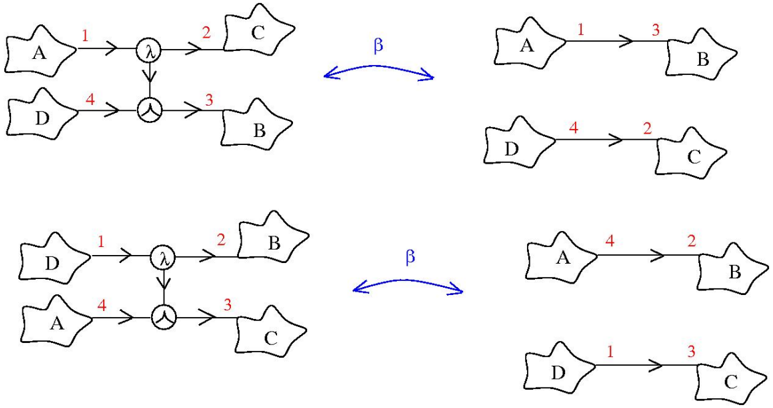
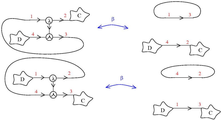
Also, we can apply in different ways a graphic beta move, to the same graph and in the
same place, simply by using different labels '1', ... '4' (here A , B , C , D are graphs in GRAPH ):
A particular case of the previous figure is yet another justification for having loops as elements in GRAPH .
<details>
<summary>Image 8 Details</summary>
### Visual Description
## Diagram: Network Transformation with β Operator
### Overview
The image presents two interconnected diagrams illustrating a network transformation process mediated by a β operator. Each diagram consists of four nodes (A, B, C, D) connected by labeled pathways (1-4), with a central λ node acting as an intermediary. The β operator (blue bidirectional arrows) indicates a reversible transformation between the two network configurations.
### Components/Axes
- **Nodes**:
- A, B, C, D (represented as irregular polygons)
- λ (central circular node with bidirectional arrows)
- **Pathways**:
- Labeled 1-4 (red numerals) indicating directional connections
- β operator (blue bidirectional arrows) between diagrams
- **Flow Direction**:
- Top diagram: A→λ→C (1→2), D→λ→B (4→3)
- Bottom diagram: A→B (4→2), D→C (1→3)
- **Transformation**:
- β operator connects top and bottom diagrams bidirectionally
### Detailed Analysis
1. **Top Diagram Configuration**:
- A connects to λ via pathway 1 (A→λ)
- λ connects to C via pathway 2 (λ→C)
- D connects to λ via pathway 4 (D→λ)
- λ connects to B via pathway 3 (λ→B)
2. **Bottom Diagram Configuration**:
- A connects directly to B via pathway 4 (A→B)
- D connects directly to C via pathway 1 (D→C)
- Pathways 2 and 3 are absent in this configuration
3. **β Operator Function**:
- Reversible transformation between configurations
- Preserves pathway numbering but alters node connections
- Suggests permutation of network topology
### Key Observations
- Pathway 4 maintains consistent directionality (A→B in bottom, D→λ in top)
- Pathway 1 changes from A→λ (top) to D→C (bottom)
- Central λ node disappears in bottom configuration
- β operator enables bidirectional network reconfiguration
### Interpretation
This diagram illustrates a network reconfiguration process where the β operator facilitates:
1. **Topological Permutation**: Rearrangement of node connections while preserving pathway labels
2. **Central Node Elimination**: The λ node's role is bypassed in the transformed network
3. **Directional Consistency**: Some pathways maintain their original directionality despite network changes
The transformation suggests a system capable of dynamic reconfiguration while maintaining certain operational constraints (pathway numbering). The disappearance of the central λ node in the transformed state implies a shift from a hub-and-spoke model to a more direct peer-to-peer configuration. The β operator's bidirectional nature indicates the process is reversible, allowing the network to toggle between these two states.
</details>
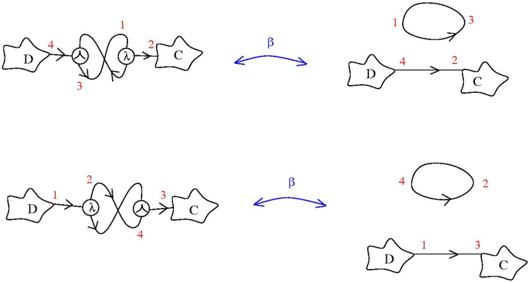
These two applications of the graphic beta move may be represented alternatively like this:
<details>
<summary>Image 9 Details</summary>
### Visual Description
## Diagram: Process Flow with Bidirectional Transformation
### Overview
The image depicts two interconnected diagrams labeled with nodes (C, D), directional arrows (1-4), and symbolic elements (λ, β). A bidirectional arrow labeled β connects the diagrams, suggesting a reversible relationship or transformation between them.
### Components/Axes
- **Nodes**:
- **C**: Star-shaped node (appears in both diagrams).
- **D**: Star-shaped node (appears in both diagrams).
- **Arrows**:
- **1, 2, 3, 4**: Numeric labels on directional arrows.
- **Symbols**:
- **λ**: Circular node with a lambda symbol (appears in both diagrams).
- **β**: Bidirectional arrow connecting the two diagrams.
- **Diagram Structure**:
- **Left Diagram**: Complex loop with nodes C, D, and λ. Arrows 1-4 form a cyclical path.
- **Right Diagram**: Simplified loop with nodes C and D. Arrows 4 and 2 form a direct path.
### Detailed Analysis
- **Left Diagram**:
- Arrows 1 (C → λ), 2 (λ → D), 3 (D → λ), 4 (λ → C) create a closed loop.
- The λ node acts as an intermediary between C and D.
- **Right Diagram**:
- Arrows 4 (D → C) and 2 (C → D) form a direct bidirectional loop between C and D.
- **Bidirectional Arrow (β)**:
- Connects the left and right diagrams, implying a transformation or equivalence between the two processes.
### Key Observations
1. The left diagram includes an additional intermediary node (λ), while the right diagram simplifies the flow directly between C and D.
2. Arrows 1-4 in the left diagram suggest a multi-step process, whereas arrows 2 and 4 in the right diagram imply a streamlined interaction.
3. The β arrow’s bidirectional nature indicates a reversible relationship, possibly denoting symmetry or equivalence.
### Interpretation
The diagrams likely represent two workflows or processes:
- **Left Diagram**: A multi-stage process involving an intermediary (λ) to mediate interactions between C and D.
- **Right Diagram**: A direct, bidirectional interaction between C and D, bypassing the intermediary.
- **β Connection**: Suggests that the two processes are interchangeable or that λ can be omitted in certain contexts.
The numeric labels (1-4) may indicate priority, sequence, or resource allocation, but without additional context, their exact meaning remains speculative. The simplification from the left to the right diagram highlights a potential optimization or abstraction of the process.
</details>
<details>
<summary>Image 10 Details</summary>
### Visual Description
## Diagram: Bidirectional System Interaction with Feedback Loops
### Overview
The image depicts two interconnected diagrams representing systems or processes labeled **D** (left) and **C** (right), linked by a bidirectional arrow labeled **β**. Each diagram contains nested loops with numbered components (1–4) and directional arrows labeled **λ**. The diagrams suggest a relationship between **D** and **C** mediated by feedback mechanisms.
---
### Components/Axes
- **Nodes/Entities**:
- **D**: Left-side system/component.
- **C**: Right-side system/component.
- **Arrows**:
- **λ**: Unidirectional arrows within each diagram (top and bottom loops).
- **β**: Bidirectional arrow connecting **D** and **C** between diagrams.
- **Labels**:
- Numbers **1–4** annotate loops in both diagrams.
- Greek letter **λ** marks internal directional flows.
---
### Detailed Analysis
#### Top Diagram:
1. **Loop Structure**:
- **D → λ → Loop 1 → λ → Loop 2 → λ → C**.
- Numbers **1, 2, 3, 4** label transitions within the loop.
2. **Flow**:
- Input from **D** enters a nested loop (1→2→3→4) before exiting to **C**.
#### Bottom Diagram:
1. **Loop Structure**:
- **D → λ → Loop 1 → λ → Loop 2 → λ → C**.
- Numbers **1, 2, 3, 4** label transitions, but the loop order differs (e.g., 4→2 in the final loop).
2. **Flow**:
- Input from **D** traverses a modified loop (1→2→3→4) before exiting to **C**.
#### Bidirectional Connection (β):
- **β** links the two diagrams, implying mutual influence or exchange between **D** and **C**.
---
### Key Observations
1. **Loop Variations**:
- The top and bottom diagrams share similar loop structures but differ in numerical labeling (e.g., **4→2** in the bottom diagram vs. **3→4** in the top).
2. **Bidirectional β**:
- The **β** arrow suggests **D** and **C** interact reciprocally, possibly indicating feedback or synchronization.
3. **λ Arrows**:
- Unidirectional **λ** arrows within loops imply sequential processing or transformation steps.
---
### Interpretation
- **System Dynamics**:
The diagrams likely model a process where **D** and **C** are interdependent systems. The nested loops (1–4) represent stages of transformation or feedback within each system, while **β** enables cross-system interaction.
- **Functional Relationships**:
- **λ** arrows denote directional causality (e.g., **D** influences **C** via intermediate steps).
- **β** suggests **C** can also influence **D**, creating a closed-loop system.
- **Anomalies**:
The differing numerical labels in the loops (e.g., **4→2** vs. **3→4**) may indicate alternative pathways or conditional logic within the systems.
---
### Conclusion
This diagram illustrates a bidirectional relationship between **D** and **C**, mediated by nested feedback loops. The use of **λ** and **β** highlights directional and reciprocal interactions, respectively. The numerical labels (1–4) likely encode process steps or component dependencies, with variations between diagrams suggesting adaptability or alternative states in the system.
</details>
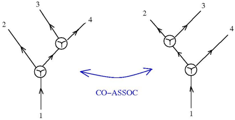
- 2.2. (CO-ASSOC) move. This is the 'co-associativity' move involving the Υ graphs. We think about the Υ graph as corresponding to a FAN-OUT gate.
<details>
<summary>Image 11 Details</summary>
### Visual Description
## Diagram: Directed Graph with Co-Association Relationship
### Overview
The image depicts two mirrored directed graphs connected by a bidirectional arrow labeled "CO-ASSOC". Each graph consists of nodes labeled 1, 2, 3, and 4, with arrows indicating directional relationships. Central nodes in both graphs feature a "Y" symbol, suggesting a decision or branching point.
### Components/Axes
- **Nodes**:
- Left graph: Nodes labeled 1 (root), 2, 3, 4.
- Right graph: Nodes labeled 1 (root), 2, 3, 4.
- **Arrows**:
- Left graph: Arrows from 1→2, 1→3, 3→4.
- Right graph: Arrows from 1→2, 1→3, 3→4.
- **Central Symbol**: "Y" in both graphs, positioned at the intersection of arrows.
- **Connecting Element**: Bidirectional arrow labeled "CO-ASSOC" between the two graphs.
### Detailed Analysis
- **Left Graph**:
- Node 1 branches to nodes 2 and 3.
- Node 3 further branches to node 4.
- **Right Graph**:
- Mirrored structure: Node 1 branches to nodes 2 and 3.
- Node 3 branches to node 4.
- **CO-ASSOC Relationship**:
- The bidirectional arrow implies a mutual association or equivalence between the two graphs.
### Key Observations
1. **Symmetry**: Both graphs share identical structural patterns (1→2, 1→3, 3→4).
2. **Central "Y" Nodes**: Positioned at the convergence of arrows, possibly representing decision nodes or critical junctions.
3. **CO-ASSOC Label**: Explicitly defines the relationship between the two graphs, suggesting they are interdependent or equivalent in function.
### Interpretation
The diagrams likely represent a system or process where two equivalent structures (left and right graphs) are mutually associated. The "Y" nodes may symbolize decision points or critical nodes in the flow. The co-association implies that the behavior or properties of one graph are mirrored or dependent on the other. This could model scenarios such as parallel processes, mirrored decision trees, or systems with redundant pathways.
**Note**: No numerical data or quantitative trends are present; the focus is on structural relationships and symbolic labels.
</details>
By using CO-ASSOC moves, we can move between any two binary trees formed only with Υ gates, with the same number of output leaves.
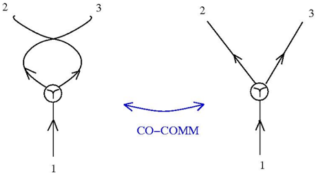
- 2.3. (CO-COMM) move. This is the 'co-commutativity' move involving the Υ gate. It will be not used until the section 6 concerning knot diagrams.
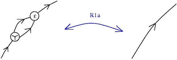
- 2.3.a (R1a) move. This move is imported from emergent algebras. Explanations are given in section 5. It involves an Υ graph and a ¯ ε graph, with ε ∈ Γ.
<details>
<summary>Image 12 Details</summary>
### Visual Description
## Diagram: Process Flow Comparison
### Overview
The image depicts two interconnected diagrams labeled "CO-COMM" (communication) via a bidirectional blue arrow. The left diagram shows a cyclic process with feedback loops, while the right diagram illustrates a linear branching process. Both share a central node with three labeled arrows (1, 2, 3).
### Components/Axes
- **Left Diagram**:
- Central node with three outgoing arrows:
- Arrow 1: Downward (linear path).
- Arrows 2 and 3: Curved upward, forming a feedback loop back to the central node.
- No explicit axis labels or scales.
- **Right Diagram**:
- Central node with three diverging arrows:
- Arrow 1: Downward (linear path).
- Arrows 2 and 3: Branching upward at 45° angles.
- No explicit axis labels or scales.
- **Connecting Element**:
- Blue bidirectional arrow labeled "CO-COMM" between the two diagrams.
### Detailed Analysis
- **Left Diagram**:
- Arrows 2 and 3 create a closed loop, suggesting iterative or recursive behavior.
- Arrow 1 represents a terminal or output path.
- **Right Diagram**:
- Arrows 2 and 3 diverge independently, indicating parallel or branching workflows.
- Arrow 1 mirrors the left diagram’s linear path.
- **CO-COMM Arrow**:
- Positioned centrally between the diagrams, implying bidirectional interaction or synchronization between the two processes.
### Key Observations
1. The left diagram emphasizes cyclical feedback (arrows 2/3), while the right prioritizes linear divergence (arrows 2/3).
2. Arrow 1 in both diagrams acts as a common output or termination point.
3. No numerical data or quantitative labels are present; the focus is on structural relationships.
### Interpretation
The diagrams likely represent two contrasting process models:
- **Left (Cyclic)**: Suitable for systems requiring continuous feedback (e.g., control loops, iterative algorithms).
- **Right (Linear)**: Represents decision trees or workflows with parallel paths.
- **CO-COMM**: Suggests these models interact or share information, possibly in hybrid systems (e.g., combining feedback with branching logic).
No numerical trends or outliers exist due to the absence of quantitative data. The diagrams emphasize structural logic over measurable metrics.
</details>
<details>
<summary>Image 13 Details</summary>
### Visual Description
## Diagram: Bidirectional System Interaction
### Overview
The image depicts two interconnected diagrams linked by a bidirectional arrow labeled "R1a". The left diagram contains two nodes with symbols "ε" and "Y", while the right diagram contains a single node with a "T" symbol. Arrows indicate directional relationships between components.
### Components/Axes
- **Left Diagram**:
- Node 1: Circular node with "ε" (epsilon) symbol
- Node 2: Circular node with "Y" symbol (resembling a branching point)
- Arrows: Multiple directional arrows connecting nodes
- **Right Diagram**:
- Node: Single node with "T" symbol
- **Connecting Element**:
- Bidirectional arrow labeled "R1a" between diagrams
### Detailed Analysis
- **Left Diagram**:
- "ε" node appears to be a source or origin point
- "Y" node shows branching structure with three outgoing arrows
- Arrows form a closed loop between the two nodes
- **Right Diagram**:
- "T" node has two outgoing arrows
- Positioned separately from left diagram
- **R1a Relationship**:
- Bidirectional connection between diagrams
- Suggests two-way interaction between systems
### Key Observations
1. The "Y" node in the left diagram acts as a decision point with multiple pathways
2. The "T" node in the right diagram appears to be a terminal or target node
3. The bidirectional "R1a" connection implies mutual influence between systems
4. Closed loop in left diagram suggests cyclical processes
### Interpretation
This diagram likely represents a system architecture where:
- The left diagram shows an error/exception handling system ("ε") interacting with a decision-making process ("Y")
- The right diagram represents a target system ("T") that both receives and sends information
- "R1a" could represent a communication protocol or data exchange mechanism
- The closed loop in the left diagram indicates feedback mechanisms within the error/exception system
- The branching structure of "Y" suggests multiple possible outcomes or processing paths
The bidirectional relationship implies that decisions from the "Y" node affect the target system "T", while feedback from "T" influences the decision-making process. This could represent a control system with error correction and adaptive decision-making capabilities.
</details>
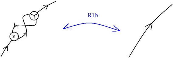
2.3.b (R1b) move. The move R1b (also related to emergent algebras) is this:
<details>
<summary>Image 14 Details</summary>
### Visual Description
## Diagram: Process Flow with R1b Transformation
### Overview
The diagram illustrates a two-part process flow. On the left, a complex cyclic structure with labeled nodes (ε and Y) is connected via directional arrows. On the right, a simplified linear pathway with a forked arrow is depicted. A blue bidirectional arrow labeled "R1b" bridges the two sections, suggesting a relationship or transformation between them.
### Components/Axes
- **Left Diagram**:
- **Nodes**:
- Circle labeled "ε" (epsilon) with inward-pointing arrows.
- Circle with a "Y" symbol (possibly representing a branching or decision point) with outward-pointing arrows.
- **Flow**:
- Arrows form a closed loop, indicating cyclical or recursive behavior.
- **Right Diagram**:
- **Pathway**:
- Straight line with a forked arrow at the end, suggesting divergence or branching.
- **Connecting Element**:
- Blue bidirectional arrow labeled "R1b" spans the gap between the left and right diagrams, implying a bidirectional relationship or transformation.
### Detailed Analysis
- **Left Diagram**:
- The "ε" node acts as a central hub with inward arrows, possibly representing accumulation or convergence.
- The "Y" node functions as a source or decision point, with arrows radiating outward, indicating divergence or branching.
- The cyclical loop suggests a feedback mechanism or iterative process.
- **Right Diagram**:
- The linear pathway with a forked arrow implies a progression toward a decision point or outcome.
- **R1b Arrow**:
- The bidirectional nature of "R1b" suggests a reversible or bidirectional interaction between the complex left structure and the simplified right pathway.
### Key Observations
1. The "R1b" label is the only textual element explicitly connecting the two diagrams, emphasizing its role as a critical link.
2. The left diagram’s cyclical structure contrasts with the right diagram’s linear pathway, highlighting a transformation from complexity to simplicity.
3. The "Y" symbol and forked arrow on the right may represent analogous concepts (e.g., branching in both cases), but their exact relationship requires further context.
### Interpretation
The diagram likely represents a scientific or technical process where a complex, cyclical system (left) undergoes a transformation mediated by "R1b" to produce a simpler, linear outcome (right). The "ε" node could symbolize a conserved quantity or energy state, while the "Y" node might represent a catalytic or decision-making step. The bidirectional "R1b" arrow implies that the transformation is not unidirectional, allowing for feedback or reversibility. This structure is common in fields like biochemistry (e.g., metabolic pathways), systems engineering, or decision-tree modeling, where complex interactions simplify into actionable outcomes.
</details>
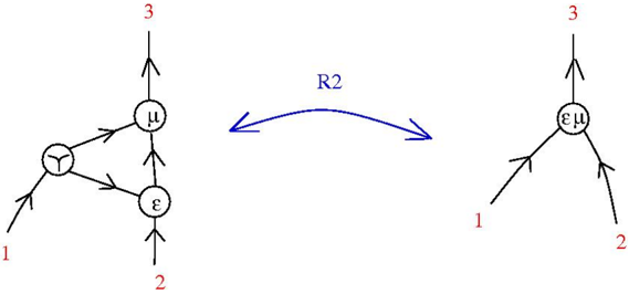
2.4. (R2) move. This corresponds to the Reidemeister II move for emergent algebras. It involves an Υ graph and two other: a ¯ ε and a ¯ µ graph, with ε, µ ∈ Γ.
<details>
<summary>Image 15 Details</summary>
### Visual Description
## Diagram: System Transformation via Rule R2
### Overview
The image depicts two interconnected diagrams labeled with nodes and directional arrows. A bidirectional arrow labeled "R2" connects the left and right diagrams, suggesting a transformation or relationship between the two systems. The left diagram is more complex, while the right is simplified.
### Components/Axes
- **Left Diagram**:
- Nodes labeled: `μ`, `ε`, `1`, `2`, `3`.
- Arrows indicate directional relationships:
- `μ` → `ε` (top to bottom).
- `ε` → `1` (bottom to left).
- `ε` → `2` (bottom to right).
- `1` → `μ` (left to top).
- `2` → `μ` (right to top).
- `3` → `μ` (top to top).
- **Right Diagram**:
- Nodes labeled: `μ`, `ε`, `1`, `2`, `3`.
- Arrows indicate directional relationships:
- `μ` → `1` (top to left).
- `μ` → `2` (top to right).
- `ε` → `3` (bottom to top).
- **Connecting Element**:
- Bidirectional arrow labeled "R2" between the diagrams.
### Detailed Analysis
- **Left Diagram**:
- `μ` acts as a central hub receiving inputs from `1`, `2`, and `3`, while also sending output to `ε`.
- `ε` distributes outputs to `1` and `2`, with `1` and `2` feeding back into `μ`.
- `3` directly influences `μ` without intermediate steps.
- **Right Diagram**:
- `μ` directly controls `1` and `2`, bypassing `ε`.
- `ε` directly influences `3`, which feeds into `μ`.
- **R2 Relationship**:
- The bidirectional arrow implies a reversible transformation or equivalence between the two systems under rule R2.
### Key Observations
1. **Complexity Reduction**: The right diagram simplifies the left by removing intermediate steps (e.g., `ε` is no longer a hub for `1` and `2`).
2. **Central Role of `μ`**: In both diagrams, `μ` is a critical node, acting as a central processor or controller.
3. **Bidirectional R2**: The reversible nature of R2 suggests the transformation can be applied in both directions, preserving system integrity.
### Interpretation
The diagrams likely represent a system where rule R2 enables simplification or optimization. The left diagram may model a detailed, multi-step process, while the right diagram reflects a streamlined version. The preservation of `μ` and `ε` across both diagrams indicates these components are fundamental to the system’s functionality. The bidirectional R2 arrow implies that the transformation is not one-way, allowing for dynamic adjustments between complexity and simplicity. This could relate to computational models, workflow optimization, or theoretical frameworks where rules govern state transitions.
</details>
This move appears in section 3.4, p. 21 [6], with the supplementary name 'triangle move'.
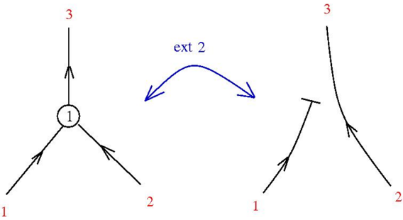
- 2.5. (ext2) move. This corresponds to the rule (ext2) from λ -Scale calculus, it expresses the fact that in emergent algebras the operation indexed with the neutral element 1 of the group Γ has the property x ◦ 1 y = y .
<details>
<summary>Image 16 Details</summary>
### Visual Description
## Diagram: State Transition and Extension Process
### Overview
The image contains two interconnected diagrams separated by a bidirectional arrow labeled "ext 2". The left diagram shows a central node (1) with three outgoing arrows to nodes labeled 1, 2, and 3. The right diagram depicts a modified structure with a split in the central connection, maintaining labels 1, 2, and 3 but altering the flow dynamics.
### Components/Axes
- **Left Diagram**:
- Central node labeled "1" (circular, bold)
- Three outgoing arrows:
- Direct upward arrow to node "3"
- Diagonal left arrow to node "1"
- Diagonal right arrow to node "2"
- **Right Diagram**:
- Central node split into two branches:
- Left branch: Direct upward arrow to node "3"
- Right branch: Curved arrow to node "2"
- Node "1" appears disconnected from the central split
- **Connecting Element**:
- Bidirectional curved arrow labeled "ext 2" between diagrams
### Detailed Analysis
- **Left Diagram**:
- Node "1" acts as a source with three possible transitions
- Arrows maintain consistent thickness and directionality
- Node labels use red numerals (1, 2, 3)
- **Right Diagram**:
- Central connection bifurcates, creating asymmetry
- Node "1" is isolated from the main flow
- Arrows show varied curvature (straight vs. curved)
- **Connecting Arrow**:
- "ext 2" suggests an extension/transformation operation
- Bidirectional nature implies reversible process
### Key Observations
1. Structural asymmetry between diagrams despite identical node labels
2. Node "1" undergoes positional change (central → peripheral)
3. Connection patterns evolve from radial to bifurcated
4. "ext 2" implies a second-order transformation or extension
### Interpretation
The diagrams appear to represent state transitions in a system, with "ext 2" denoting a specific operation that:
1. Reconfigures central node relationships
2. Introduces hierarchical separation between nodes
3. Alters flow dynamics through directional changes
4. Maintains core node identities while modifying interactions
The transformation suggests a controlled modification process where:
- Node "1" loses its central role
- Node "3" gains prominence through direct connection
- Node "2" becomes the terminal state
- The system gains configurational complexity through the extension operation
</details>
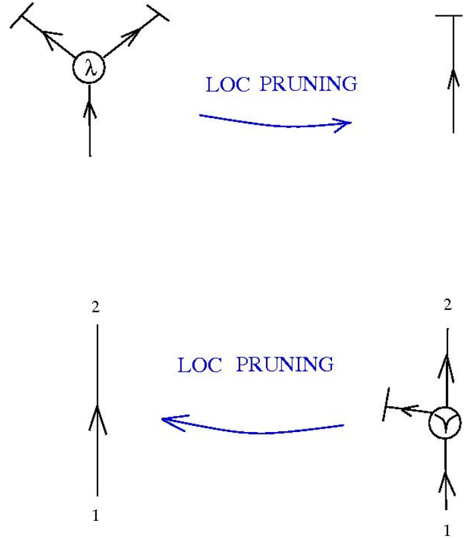
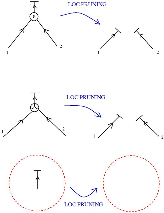
2.6. Local pruning. Local pruning moves are local moves which eliminate 'dead' edges. Notice that, unlike the previous moves, these are one-way (you can eliminate dead edges, but not add them to graphs).
<details>
<summary>Image 17 Details</summary>
### Visual Description
## Diagram: LOC PRUNING Process Flow
### Overview
The image contains two interconnected diagrams illustrating a "LOC PRUNING" process. Both diagrams use directional arrows and labeled nodes to represent transformations. The diagrams are connected by a blue arrow labeled "LOC PRUNING," indicating a sequential or iterative process.
---
### Components/Axes
1. **Top Diagram**:
- **Central Node**: Labeled `λ` (lambda), with three outgoing arrows:
- Two arrows branching left and right (horizontal divergence).
- One arrow pointing downward (vertical continuation).
- **Arrows**: Black lines with arrowheads indicating direction.
- **Text**: "LOC PRUNING" in blue, positioned below the diagram with an arrow pointing to the right.
2. **Bottom Diagram**:
- **Vertical Line**: Labeled `1` (bottom) and `2` (top), suggesting hierarchical levels or steps.
- **Horizontal Arrow**: Points leftward from the vertical line, labeled "LOC PRUNING."
- **Final Node**: A `Y`-shaped node with two outgoing arrows (left and right divergence).
- **Arrows**: Black lines with arrowheads.
---
### Detailed Analysis
- **Top Diagram**:
- The `λ` node acts as a source or decision point, splitting into two paths (left/right) while maintaining a downward path.
- The "LOC PRUNING" label and arrow suggest a transformation or filtering step applied to this structure.
- **Bottom Diagram**:
- The vertical line (`1` to `2`) may represent a prioritized or ordered sequence.
- The leftward arrow from the vertical line indicates a reversal or reorientation of flow.
- The `Y`-shaped node introduces a new divergence, possibly representing optimized or simplified pathways after pruning.
---
### Key Observations
1. **Process Flow**:
- The top diagram’s `λ` node undergoes "LOC PRUNING," resulting in the bottom diagram’s restructured `Y`-shaped node.
- The vertical labels (`1`, `2`) imply a two-stage process or prioritization.
2. **Structural Changes**:
- The top diagram’s horizontal divergence is replaced by a vertical hierarchy in the bottom diagram.
- The final `Y`-shaped node retains divergence but in a different orientation, suggesting selective path retention.
3. **No Numerical Data**:
- The diagrams lack quantitative values, focusing instead on symbolic representation of flow and structure.
---
### Interpretation
The diagrams depict a **LOC PRUNING** process that simplifies or optimizes a branching structure. The top diagram represents an initial complex configuration (`λ` node with multiple paths), while the bottom diagram shows a streamlined outcome after pruning. Key insights:
- **Pruning Mechanism**: The process removes redundant or low-priority paths (e.g., the top diagram’s horizontal divergence is replaced by a vertical hierarchy).
- **Hierarchical Optimization**: The vertical labels (`1`, `2`) may indicate prioritization, with higher-level paths (`2`) retained after pruning.
- **Flow Reorientation**: The leftward arrow in the bottom diagram suggests a reversal of direction, possibly to align with downstream requirements.
This process could model computational optimizations (e.g., reducing decision trees), resource allocation, or workflow simplification in technical systems.
</details>
<details>
<summary>Image 18 Details</summary>
### Visual Description
## Diagram: LOC PRUNING Process
### Overview
The image depicts a two-stage process labeled "LOC PRUNING" involving hierarchical structures. It shows a transformation from complex branching systems to simplified configurations through iterative pruning operations. The diagram uses directional arrows, labeled components, and geometric shapes to represent the workflow.
### Components/Axes
1. **Upper Section**:
- **Left Diagram**:
- Central circle labeled "ε" (epsilon)
- Two downward arrows labeled "1" and "2"
- Vertical line with bidirectional arrow (top-down)
- **Right Diagram**:
- Two isolated vertical lines labeled "1" and "2"
- No central connecting node
- **Connecting Element**: Blue curved arrow labeled "LOC PRUNING" between left and right diagrams
2. **Lower Section**:
- Two red dashed circles connected by a blue curved arrow labeled "LOC PRUNING"
- Each circle contains:
- Vertical line with unidirectional arrow (top-down)
- No branching elements
### Detailed Analysis
- **Upper Left Diagram**: Represents an initial hierarchical structure with a central node (ε) distributing outputs to two branches (1 and 2). The bidirectional arrow suggests potential feedback or bidirectional relationships.
- **Upper Right Diagram**: Shows the result of pruning, where the central node is removed, leaving only the two branches (1 and 2) as independent entities.
- **Lower Section**: Illustrates a further simplification stage where the pruned branches are encapsulated in isolated circular structures with unidirectional flow, suggesting finalized or stabilized states.
### Key Observations
1. **Pruning Mechanism**: The blue "LOC PRUNING" arrows indicate a systematic removal of intermediate nodes (ε) while preserving terminal branches (1 and 2).
2. **Structural Simplification**: Each pruning step reduces complexity:
- Stage 1: Removes central node (ε)
- Stage 2: Encapsulates branches in isolated structures
3. **Flow Direction**: All arrows point downward, emphasizing a top-down processing or decision-making flow.
### Interpretation
This diagram likely represents a computational or algorithmic process for optimizing hierarchical structures. The "LOC PRUNING" operation appears to:
1. Eliminate redundant decision points (ε)
2. Preserve essential pathways (1 and 2)
3. Stabilize the system through encapsulation (red circles)
The progression from complex branching to isolated components suggests an optimization strategy that balances efficiency (reduced complexity) with functionality (preserved critical paths). The use of bidirectional arrows in the initial stage versus unidirectional arrows in the final stage may indicate a transition from exploratory to deterministic processing.
No numerical data or quantitative metrics are present in the diagram. The focus is entirely on structural relationships and transformation logic rather than measurable values.
</details>
Global moves or conditions. Global moves are those which are not local, either because the condition C applies to parts of the graph which may have an arbitrary large sum or edges plus nodes, or because after the move the graph P ′ which replaces the graph P has an arbitrary large sum or edges plus nodes.
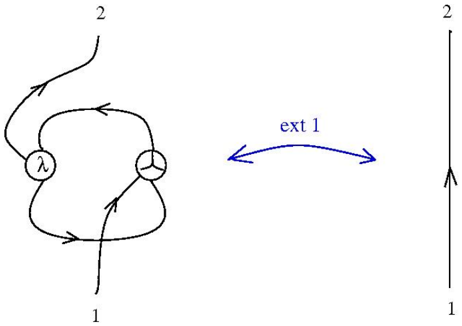
2.7. (ext1) move. This corresponds to the rule (ext1) from λ -Scale calculus, or to η -reduction in lambda calculus (see theorem 3.1, part (e) for details). It involves a λ graph (think about the λ abstraction operation in lambda calculus) and a graph (think about the application operation in lambda calculus).
The rule is: if there is no oriented path from '2' to '1', then the following move can be performed.
<details>
<summary>Image 19 Details</summary>
### Visual Description
## Diagram: Cyclic System with Linear Extension
### Overview
The image depicts a technical diagram with two distinct components:
1. A **looped structure** on the left containing two labeled nodes (`λ` and `μ`) connected by directional arrows forming a closed cycle.
2. A **vertical line** on the right with directional arrows at the top and bottom labeled `2` and `1`, respectively.
A bidirectional arrow labeled `ext 1` connects the looped structure to the vertical line, suggesting an interaction or extension between the two systems.
### Components/Axes
- **Looped Structure**:
- Nodes:
- Left node labeled `λ` (Greek letter lambda).
- Right node labeled `μ` (Greek letter mu).
- Arrows:
- Four directional arrows forming a closed loop between `λ` and `μ`.
- Arrows are unlabeled but imply cyclical flow.
- **Vertical Line**:
- A single vertical line with two directional arrows:
- Top arrow labeled `2` (pointing upward).
- Bottom arrow labeled `1` (pointing downward).
- **Connection**:
- A bidirectional arrow labeled `ext 1` links the looped structure to the vertical line.
### Detailed Analysis
- **Looped Structure**:
- The cycle between `λ` and `μ` suggests a feedback or iterative process.
- No numerical values or additional labels are present on the arrows or nodes.
- **Vertical Line**:
- The labels `2` (top) and `1` (bottom) may indicate hierarchical levels, states, or positions.
- The directional arrows imply a unidirectional flow (upward and downward).
- **Connection (`ext 1`)**:
- The bidirectional arrow `ext 1` implies a two-way interaction or extension between the looped system and the linear system.
### Key Observations
1. The looped structure (`λ` ↔ `μ`) represents a self-contained cyclic process.
2. The vertical line (`2` ↔ `1`) represents a linear, hierarchical, or sequential system.
3. The `ext 1` connection suggests the looped system is extended or integrated with the linear system.
### Interpretation
This diagram likely models a system where:
- **Cyclic processes** (e.g., feedback loops, iterative workflows) interact with **linear hierarchies** (e.g., decision trees, state transitions).
- The `ext 1` label indicates a critical interface or dependency between the two subsystems.
- The absence of numerical data or units suggests the diagram is conceptual, focusing on structural relationships rather than quantitative metrics.
**Notable Patterns**:
- The looped structure’s symmetry implies balanced interactions between `λ` and `μ`.
- The vertical line’s asymmetry (top `2`, bottom `1`) may denote a priority or directional preference.
- The bidirectional `ext 1` arrow highlights a non-hierarchical, mutual relationship between the systems.
**Underlying Implications**:
- The diagram could represent a technical workflow, such as a software architecture where a cyclical module (`λ`/`μ`) extends a linear process (`ext 1`).
- Alternatively, it might model a biological or physical system with feedback loops and linear pathways.
- The lack of explicit data points or units leaves the interpretation open to domain-specific context.
</details>
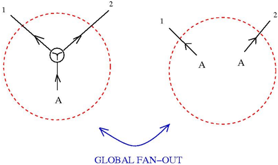
2.8. (Global FAN-OUT) move. This is a global move, because it consists in replacing (under certain circumstances) a graph by two copies of that graph.
The rule is: if a graph in G ∈ GRAPH has a Υ bottleneck, that is if we can find a sub-graph A ∈ GRAPH connected to the rest of the graph G only through a Υ gate, then we can perform the move explained in the next figure, from the left to the right.
Conversely, if in the graph G we can find two identical subgraphs (denoted by A ), which are in GRAPH , which have no edge connecting one with another and which are connected to the rest of G only through one edge, as in the RHS of the figure, then we can perform the move from the right to the left.
<details>
<summary>Image 20 Details</summary>
### Visual Description
## Diagram: Global Fan-Out Process Flow
### Overview
The image depicts two interconnected diagrams illustrating a data flow or process transformation labeled "GLOBAL FAN-OUT." The left diagram (Diagram 1) shows a central node with three outgoing arrows, while the right diagram (Diagram 2) shows two incoming arrows converging on a labeled point. A blue bidirectional arrow connects the diagrams, emphasizing the global nature of the process.
### Components/Axes
- **Diagram 1 (Left)**:
- Central node with three outgoing arrows labeled **1**, **2**, and **A**.
- Enclosed in a red dashed circle.
- **Diagram 2 (Right)**:
- Two incoming arrows labeled **1** and **2**, both pointing to a labeled point **A**.
- Enclosed in a red dashed circle.
- **Global Connection**:
- Blue bidirectional arrow labeled **"GLOBAL FAN-OUT"** connects Diagram 1 and Diagram 2.
- **Text Elements**:
- "GLOBAL FAN-OUT" in uppercase blue text at the bottom center.
### Detailed Analysis
- **Diagram 1**:
- The central node acts as a source or origin point.
- Arrows **1** and **2** likely represent distinct data streams or processes.
- Arrow **A** may indicate a third process or output originating from the same node.
- **Diagram 2**:
- Arrows **1** and **2** converge on point **A**, suggesting aggregation, merging, or transformation of inputs into a unified output.
- The red dashed circle implies a boundary or processing stage.
- **Global Fan-Out**:
- The blue arrow indicates bidirectional interaction or synchronization between the two diagrams.
- The term "FAN-OUT" suggests a distribution or expansion of data/processes from a central point.
### Key Observations
1. **Reduction in Outputs**: Diagram 1 has three outputs (1, 2, A), while Diagram 2 consolidates two inputs into a single output (A).
2. **Symmetry in Labeling**: Both diagrams use labels **1**, **2**, and **A**, but their roles differ (outputs vs. inputs).
3. **Bidirectional Flow**: The blue arrow implies a feedback loop or mutual dependency between the diagrams.
### Interpretation
The diagram likely represents a system where:
- **Diagram 1** models the initial distribution or generation of processes/data streams (1, 2, A).
- **Diagram 2** represents a subsequent stage where these streams are filtered, merged, or transformed into a unified output (A).
- The "GLOBAL FAN-OUT" mechanism ensures coordination or synchronization between the initial distribution and final convergence, possibly indicating a distributed computing architecture or data pipeline.
The use of identical labels (**1**, **2**, **A**) in both diagrams suggests a cyclical or iterative process, where outputs from one stage become inputs for another. The red dashed circles may symbolize isolated processing units or stages within a larger system.
</details>
Remark that (global FAN-OUT) trivially implies (CO-COMM). ( As an local rule alternative to the global FAN-OUT, we might consider the following. Fix a number N and consider only graphs A which have at most N (nodes + arrows). The N LOCAL FAN-OUT move is the same as the GLOBAL FAN-OUT move, only it applies only to such graphs A . This local FAN-OUT move does not imply CO-COMM.)
2.9. Global pruning. This a global move which eliminates 'dead' edges.
The rule is: if a graph in G ∈ GRAPH has a ending, that is if we can find a sub-graph A ∈ GRAPH connected only to a gate, with no edges connecting to the rest of G , then we can erase this graph and the respective gate.
<details>
<summary>Image 21 Details</summary>
### Visual Description
## Diagram: System Pruning Process
### Overview
The diagram illustrates a two-stage system transformation labeled "GLOBAL PRUNING." It features two interconnected dashed circles with a directional arrow between them. The left circle contains a labeled structural component, while the right circle remains empty, suggesting a simplification or reduction process.
### Components/Axes
- **Left Circle**: Contains a vertical line with a T-shaped intersection and a downward-pointing arrow labeled "A" at its base.
- **Right Circle**: Empty dashed circle with no internal elements.
- **Connecting Arrow**: Blue arrow labeled "GLOBAL PRUNING" pointing from left to right circle.
- **No legend, axes, or numerical scales present.**
### Detailed Analysis
- **Left Circle Structure**: The T-shaped configuration with a vertical line and downward arrow suggests a hierarchical or decision-tree-like structure. The label "A" likely represents a specific node or decision point.
- **Right Circle**: Complete absence of internal elements implies a state of reduction, simplification, or elimination of all components.
- **Arrow Label**: "GLOBAL PRUNING" indicates a system-wide optimization or elimination process affecting all elements.
### Key Observations
1. The transformation from a structured system (left) to an empty state (right) occurs through global pruning.
2. The labeled component "A" in the left circle is the only explicitly marked element, suggesting it may be a critical node in the pruning process.
3. No intermediate states or transitional elements are shown between the circles.
### Interpretation
This diagram appears to represent a conceptual model of system optimization where:
- The left circle represents an initial complex system with identifiable components (specifically component A)
- "GLOBAL PRUNING" acts as a system-wide operation that removes all structural elements
- The right circle's emptiness suggests either complete elimination of components or abstraction to a minimal state
- The T-shaped structure in the left circle might represent decision points or branching logic that gets eliminated during pruning
The absence of intermediate states implies an all-or-nothing pruning approach rather than gradual simplification. The single labeled component "A" could indicate either a preserved element (if pruning is selective) or a placeholder for the system's original state before complete reduction.
</details>
The global pruning may be needed because of the λ gates, which cannot be removed only by local pruning.
2.10. Elimination of loops. It is possible that, after using a local or global move, we obtain a graph with an arrow which closes itself, without being connected to any node. Here is an example, concerning the application of the graphic β move. We may erase any such loop, or add one.
λ GRAPHS. The edges of an elementary graph λ can be numbered unambiguously, clockwise, by 1, 2, 3, such that 1 is the number of the entrant edge.
Definition 2.4 A graph G ∈ GRAPH is a λ -graph, notation G ∈ λGRAPH , if:
- -it does not have ¯ ε gates,
- -for any node λ any oriented path in G starting at the edge 2 of this node can be completed to a path which either terminates in a graph , or else terminates at the edge 1 of this node.
The condition G ∈ λGRAPH is global, in the sense that in order to decide if G ∈ λGRAPH we have to examine parts of the graph which may have an arbitrary large sum or edges plus nodes.
## 3 Conversion of lambda terms into GRAPH
Here I show how to associate to a lambda term a graph in GRAPH , then I use this to show that β -reduction in lambda calculus transforms into the β rule for GRAPH . (Thanks to Morita Yasuaki for some corrections.)
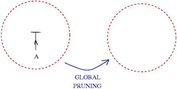
Indeed, to any term A ∈ T ( X ) (where T ( X ) is the set of lambda terms over the variable set X ) we associate its syntactic tree. The syntactic tree of any lambda term is constructed by using two gates, one corresponding to the λ abstraction and the other corresponding to the application. We draw syntactic trees with the leaves (elements of X ) at the bottom and the root at the top. We shall use the following notation for the two gates: at the left is the gate for the λ abstraction and at the right is the gate for the application.
<details>
<summary>Image 22 Details</summary>
### Visual Description
## Diagram: Lambda (λ) Transformation and Interaction Models
### Overview
The image contains two distinct diagrams illustrating abstract transformations involving a central operator labeled **λ**. Both diagrams use directional arrows to represent relationships between variables or entities. The first diagram emphasizes a transformation process, while the second focuses on interaction or combination.
---
### Components/Axes
#### Diagram 1 (Left):
- **Central Node**: A circle labeled **λ** (Greek letter lambda).
- **Input Arrows**:
- **x**: Arrows pointing *into* λ from the left.
- **A**: Arrows pointing *into* λ from the right.
- **Output Arrow**:
- **λx.A**: Arrow pointing *out of* λ toward the top, labeled as the result of the transformation.
#### Diagram 2 (Right):
- **Central Node**: A circle labeled **λ**.
- **Input Arrows**:
- **A**: Arrows pointing *into* λ from the bottom-left.
- **B**: Arrows pointing *into* λ from the bottom-right.
- **Output Arrow**:
- **AB**: Arrow pointing *out of* λ toward the top, labeled as the combined result.
---
### Detailed Analysis
#### Diagram 1:
- **Flow**:
- Inputs **x** (left) and **A** (right) are processed by **λ**, producing **λx.A** (top).
- The notation **λx.A** suggests a composition of operations, where **λ** acts on **x** and **A** to generate a new entity.
- **Interpretation**: This could represent a mathematical function, logical operation, or computational process where **λ** mediates between **x** and **A**.
#### Diagram 2:
- **Flow**:
- Inputs **A** (bottom-left) and **B** (bottom-right) are combined via **λ** to produce **AB** (top).
- The arrow labels **AB** imply a direct interaction or aggregation of **A** and **B** under the influence of **λ**.
- **Interpretation**: This resembles a binary operation (e.g., addition, multiplication, or logical AND) where **λ** acts as a mediator or operator.
---
### Key Observations
1. **Consistency of λ**: Both diagrams use **λ** as the central operator, suggesting it plays a unifying role in transformations or interactions.
2. **Directionality**: Arrows indicate unidirectional flow, emphasizing causality or dependency (e.g., inputs → output).
3. **Notation**: The use of **λx.A** and **AB** implies algebraic or symbolic manipulation, common in lambda calculus, category theory, or functional programming.
---
### Interpretation
- **Technical Context**: These diagrams likely represent concepts from lambda calculus, category theory, or functional programming.
- In lambda calculus, **λ** denotes abstraction, and **λx.A** could represent a function taking **x** and returning **A**.
- In category theory, **λ** might symbolize a natural transformation or functor, while **AB** could denote a product or coproduct.
- **Relationships**:
- Diagram 1 highlights **transformation** (input → output via λ).
- Diagram 2 emphasizes **combination** (inputs A and B → output AB via λ).
- **Anomalies**: No numerical values or scales are present, so quantitative analysis is not applicable. The focus is purely on symbolic relationships.
---
### Conclusion
The diagrams abstractly model processes where **λ** acts as a mediator or operator. Diagram 1 illustrates a unary/binary transformation, while Diagram 2 depicts a binary interaction. These could underpin formal systems in mathematics, computer science, or logic, emphasizing the role of **λ** in structuring relationships between entities.
</details>
Remark that these two gates are from the graphical alphabet of GRAPH , but the syntactic tree is decorated: at the bottom we have leaves from X . Also, remark the peculiar orientation of the edge from the left (in tree notation convention) of the λ gate. For the moment, this orientation is in contradiction with the implicit orientation (from down-up) of edges of the syntactic tree, but soon this matter will become clear.
We shall remove all leaves decorations, with the price of introducing new gates, namely Υ and gates. This will be done in a sequence of steps, detailed further. Take the syntactic tree of A ∈ T ( X ), drawn with the mentioned conventions (concerning gates and the positioning of leaves and root respectively).
We take as examples the following five lambda terms: I = λx.x , K = λx. ( λy.x ), S = λx. ( λy. ( λz. (( xz )( yz )))), Ω = ( λx. ( xx ))( λx. ( xx )) and T = ( λx. ( xy ))( λx. ( xy )).
Step 1. Elimination of bound variables, part I. Any leaf of the tree is connected to the root by an unique path.
Start from the leftmost leaf, perform the algorithm explained further, then go to the right and repeat until all leaves are exhausted. We initialize also a list B = ∅ of bound variables.
Take a leaf, say decorated with x ∈ X . To this leaf is associated a word (a list) which is formed by the symbols of gates which are on the path which connects (from the bottom-up) the leaf with the root, together with information about which way, left (L) or right (R), the path passes through the gates. Such a word is formed by the letters λ L , λ R , L , R .
If the first letter is λ L then add to the list B the pair ( x, w ( x )) formed by the variable name x , and the associated word (describing the path to follow from the respective leaf to the root). Then pass to a new leaf.
Else continue along the path to the roof. If we arrive at a λ gate, this can happen only coming from the right leg of the λ gate, thus we can find only the letter λ R . In such a case look at the variable y which decorates the left leg of the same λ gate. If x = y then add to the syntactic tree a new edge, from y to x and proceed further along the path, else proceed further. If the root is attained then pass to next leaf.
Examples: the graphs associated to the mentioned lambda terms, together with the list of bound variables, are the following.
$$\begin{aligned}
- I &= x _ { x } . x _ { y } \text { has } B = \{ ( x , y ) \mid ( x z ) ( y z ) \} \\
&= \left\{ \begin{array}{l} x _ { x } ^ { L } \cdot y _ { y } ^ { L } \times R \right\} , S = \left\{ \begin{array}{l} x _ { R } ^ { L } \cdot y _ { R } ^ { L } \times R \right\} .
\end{aligned}$$
<details>
<summary>Image 23 Details</summary>
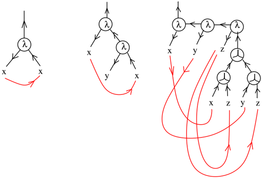
### Visual Description
## Diagram: Hierarchical Feedback System with Lambda Nodes
### Overview
The image depicts three interconnected diagrams illustrating a hierarchical system with lambda (λ) nodes, variables (x, y, z), and feedback loops. The diagrams progress from simple to complex structures, emphasizing directional relationships and recursive feedback mechanisms.
### Components/Axes
- **Nodes**:
- Lambda (λ): Central decision/processing nodes (represented as circles).
- Variables (x, y, z): Terminal nodes (represented as squares).
- **Arrows**:
- Black arrows: Primary directional flow (top-down hierarchy).
- Red arrows: Feedback loops (recursive connections from variables back to λ nodes).
- **Structure**:
- Diagrams are arranged left-to-right in increasing complexity.
- No explicit axes or scales; relationships are qualitative.
### Detailed Analysis
1. **Left Diagram**:
- Single λ node connected to two x nodes via black arrows.
- Red feedback loop connects x nodes back to λ, forming a closed loop.
- Textual labels: "λ", "x" (repeated).
2. **Middle Diagram**:
- Two λ nodes in series, with the first λ connected to x and the second to y.
- Red feedback loop connects y back to the first λ node.
- Textual labels: "λ" (repeated), "x", "y".
3. **Right Diagram**:
- Complex hierarchy with three λ nodes in series.
- First λ connects to x, second to y, third to z.
- Multiple red feedback loops:
- x → first λ
- z → second λ
- y → third λ
- z → third λ
- Textual labels: "λ" (repeated), "x", "y", "z".
### Key Observations
- **Feedback Proliferation**: The rightmost diagram shows the most feedback loops (4), suggesting increased system interdependence.
- **Variable Recursion**: Variables (x, y, z) feed back into earlier λ nodes, implying iterative processing.
- **Hierarchical Depth**: Complexity increases from 1 λ node (left) to 3 λ nodes (right), with feedback complexity scaling accordingly.
### Interpretation
This diagram represents a **recursive decision-making system** where:
1. **Lambda nodes** act as processing units that propagate decisions downward (to x, y, z).
2. **Feedback loops** enable variables to influence earlier stages, creating potential for:
- Iterative refinement (e.g., x → λ → x → λ...)
- Systemic coupling between variables and decisions.
3. The progression from left to right diagrams may symbolize:
- **Simplification to complexity**: Basic feedback (left) → Moderate coupling (middle) → Highly interconnected system (right).
- **Temporal evolution**: A system becoming more recursive over time.
The red feedback arrows are critical—they transform a static hierarchy into a dynamic, self-referential system. This could model processes like:
- Machine learning feedback cycles
- Organizational decision-making with bottom-up input
- Computational graphs with gradient backpropagation
No numerical data is present; the diagram focuses on structural relationships rather than quantitative metrics.
</details>
$$\begin{aligned}
- \Omega &= ( x _ { x } ( x _ { y } ) ) ( x _ { x } ( x _ { y } ) \\
&= \{ ( x _ { x } , λ ^ { L } , L ) , ( x _ { x } , λ ^ { L } , R ) \} , T = \{ L , R \} , \\
\lambda ^ { L } &\text{has } B = \{ ( x _ { x } , λ ^ { L } , L ) , ( x _ { x } , λ ^ { L } , R ) \}, T = \{ L , R \} .
\end{aligned}$$
Step 2. Elimination of bound variables, part II. We have now a list B of bound variables. If the list is empty then go to the next step. Else, do the following, starting from the first element of the list, until the list is finished.
<details>
<summary>Image 24 Details</summary>
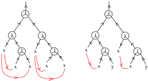
### Visual Description
## Flowchart Diagram: Branching Process with Cyclic Paths
### Overview
The image contains two identical hierarchical diagrams with branching nodes and directional arrows. Both diagrams feature a root node at the top, followed by two intermediate nodes labeled λ, which split into terminal nodes. The left diagram shows cyclic paths between terminal nodes labeled "x," while the right diagram replaces one terminal node with "y" and introduces a mixed cyclic path between "x" and "y."
### Components/Axes
- **Nodes**:
- **Root Node**: Unlabeled circle at the top.
- **Intermediate Nodes**: Two nodes labeled λ, positioned symmetrically below the root.
- **Terminal Nodes**:
- Left Diagram: Four terminal nodes labeled "x" (two under each λ).
- Right Diagram: Three terminal nodes labeled "x" and one labeled "y" (one under each λ).
- **Special Nodes**: Two nodes with a circle containing two inward-pointing arrows (likely representing feedback or cyclic states).
- **Arrows**:
- Black arrows indicate primary flow direction (top-to-bottom, left-to-right).
- Red arrows highlight cyclic paths:
- Left Diagram: Two loops connecting terminal "x" nodes.
- Right Diagram: One loop connecting "x" and "y" nodes.
### Detailed Analysis
1. **Left Diagram**:
- Root → λ₁ → x₁ → x₃ (via cyclic loop).
- Root → λ₁ → x₂ → x₄ (via cyclic loop).
- Root → λ₂ → x₅ → x₇ (via cyclic loop).
- Root → λ₂ → x₆ → x₈ (via cyclic loop).
2. **Right Diagram**:
- Root → λ₁ → x₁ → y₁ (no loop).
- Root → λ₁ → x₂ → x₄ (via cyclic loop).
- Root → λ₂ → x₅ → y₂ (no loop).
- Root → λ₂ → x₆ → x₈ (via cyclic loop).
### Key Observations
- The left diagram emphasizes self-referential cycles within "x" nodes.
- The right diagram introduces "y" as an alternative terminal state, breaking one cyclic path.
- Red arrows are positioned at the bottom of each diagram, emphasizing terminal-node interactions.
### Interpretation
The diagrams likely represent decision trees or state machines where:
- **λ Nodes**: Act as decision points or transformation stages.
- **Cyclic Paths (Red Arrows)**: Indicate feedback loops or recurring processes.
- **x vs. y Nodes**: Suggest divergent outcomes or states, with "y" representing a terminal or alternative state.
The left diagram may model a system where "x" states persistently loop, while the right diagram introduces "y" as a potential exit or resolution state. The absence of numerical data implies a qualitative representation of process flow rather than quantitative analysis.
</details>
An element, say ( x, w ( x )), of the list, is either connected to other leaves by one or more edges added at step 1, or not. If is not connected then erase the variable name with the associated path w ( x ) and replace it by a gate. If it is connected then erase it, replace it by a tree formed by Υ gates, which starts at the place where the element of the list were before the erasure and stops at the leaves which were connected to x . Erase all decorations which were joined to x and also erase all edges which were added at step 1 to the leave x from the list.
Examples: after the step 2, the graphs associated to the mentioned lambda terms are the following.
- -the graphs of I = λx.x , K = λx. ( λy.x ), S = λx. ( λy. ( λz. (( xz )( yz )))) are
- -the graphs of Ω = ( λx. ( xx ))( λx. ( xx )), T = ( λx. ( xy ))( λx. ( xy )) are
<details>
<summary>Image 25 Details</summary>
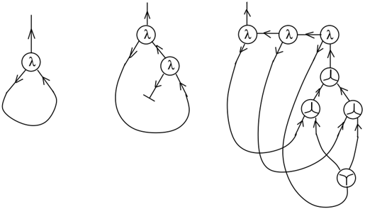
### Visual Description
## State Transition Diagrams: System Behavior Representation
### Overview
The image contains three progressively complex state transition diagrams, each illustrating system behavior through labeled nodes (circles) and directional arrows. The diagrams use the Greek letter λ (lambda) to denote states and arrows to represent transitions, with variations in arrow style indicating different transition types.
### Components/Axes
- **Nodes**:
- All nodes are labeled with the symbol λ (lambda), representing generic states.
- Nodes are depicted as circles, with some containing internal symbols (e.g., a three-pronged fork).
- **Arrows**:
- Standard arrows (→) indicate unidirectional transitions.
- Bidirectional arrows (↔) suggest reversible transitions.
- A T-shaped arrow (↑↓) appears in Diagram 2, possibly denoting a conditional or hierarchical transition.
- Loops (arrows returning to the same node) are present in all diagrams.
- **Internal Symbols**:
- A three-pronged fork () appears in Diagram 3, potentially representing a branching or parallel process.
### Detailed Analysis
#### Diagram 1 (Left)
- **Structure**: A single λ node with:
- An upward-pointing arrow (↑) from an external source to the node.
- A self-loop (→) from the node to itself.
- **Interpretation**: Represents a system with one state that can transition to itself (loop) and receives input from an external source (↑).
#### Diagram 2 (Center)
- **Structure**: Two λ nodes connected by:
- A bidirectional arrow (↔) between them.
- A T-shaped arrow (↑↓) from the top node to the bottom node.
- A self-loop on the bottom node.
- **Interpretation**: Models a two-state system with mutual transitions (↔) and a conditional or prioritized transition (↑↓) from State A to State B. The self-loop on State B suggests persistence in that state.
#### Diagram 3 (Right)
- **Structure**: Four λ nodes with:
- Multiple bidirectional (↔) and unidirectional (→) arrows.
- A three-pronged fork () in one node, splitting into three outgoing arrows.
- A loop on the bottom-right node.
- **Interpretation**: Depicts a complex system with parallel processes (), feedback loops, and conditional transitions. The fork suggests divergence into multiple pathways, while loops indicate cyclical behavior.
### Key Observations
1. **Scaling Complexity**: Diagrams increase in complexity from left to right, suggesting a progression from simple to advanced system modeling.
2. **Symbol Consistency**: The λ label is uniformly used across all diagrams, implying a shared context (e.g., states in a computational or physical system).
3. **Arrow Variants**: The introduction of T-shaped and forked arrows in later diagrams indicates expanded transition semantics (e.g., conditions, parallelism).
### Interpretation
These diagrams likely represent state machines or process flows in a technical system (e.g., software, hardware, or workflow). The use of λ as a generic state label suggests abstraction, allowing application to diverse domains. The progression from single-state to multi-state systems with branching and loops highlights increasing behavioral complexity. The T-shaped and forked arrows imply conditional logic or concurrency, critical for modeling real-world systems where transitions depend on external inputs or internal states.
No numerical data, charts, or textual content in other languages are present. The diagrams focus purely on structural and transitional relationships.
</details>
<details>
<summary>Image 26 Details</summary>
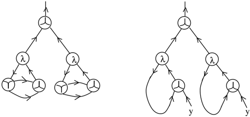
### Visual Description
## Diagram: Process Flow Comparison
### Overview
The image contains two side-by-side diagrams depicting hierarchical systems with nodes labeled "λ" (lambda) and "Y". Both diagrams show directional relationships via arrows, with the left diagram emphasizing bidirectional interactions and the right diagram incorporating feedback loops and unidirectional flows.
### Components/Axes
- **Nodes**:
- Top node: Labeled "λ" (lambda) in both diagrams.
- Intermediate nodes: Two "λ" nodes in each diagram, connected directly to the top λ.
- Bottom nodes: Three "Y" nodes in the left diagram; two "Y" nodes and a terminal "y" in the right diagram.
- **Arrows**:
- Left diagram: Bidirectional arrows between "Y" nodes (forming triangular loops).
- Right diagram: Unidirectional arrows from top λ to intermediate λ nodes, then to Y nodes. Feedback loops exist from Y nodes to the top λ, and a terminal "y" is labeled at the bottom.
### Detailed Analysis
- **Left Diagram**:
- The top λ branches into two intermediate λ nodes.
- Each intermediate λ connects to three Y nodes, which form closed triangular loops via bidirectional arrows.
- No terminal output is labeled.
- **Right Diagram**:
- The top λ branches into two intermediate λ nodes.
- Each intermediate λ connects to a single Y node.
- Y nodes have unidirectional arrows pointing back to the top λ (feedback loop).
- A terminal "y" is labeled at the bottom, suggesting an output or endpoint.
### Key Observations
1. **Bidirectional vs. Unidirectional Flow**:
- Left diagram emphasizes mutual interactions among Y nodes (bidirectional arrows).
- Right diagram introduces feedback loops (Y → top λ) and a terminal output ("y").
2. **Structural Symmetry**:
- Both diagrams share a hierarchical structure (top λ → intermediate λ → Y nodes).
- The right diagram simplifies the Y node connections (two Y nodes vs. three in the left).
3. **Terminal Output**:
- The right diagram explicitly labels a terminal "y", absent in the left diagram.
### Interpretation
- **System Behavior**:
- The left diagram likely represents a system with cyclical, interdependent processes (e.g., mutual feedback among components).
- The right diagram suggests a hierarchical system with feedback control (Y nodes regulating the top λ) and a defined output ("y").
- **Implications**:
- The bidirectional loops in the left diagram could model collaborative or competitive interactions (e.g., game theory scenarios).
- The right diagram’s feedback loop and terminal "y" might represent a regulated process with an endpoint, such as a control system or workflow.
- **Anomalies**:
- The absence of a terminal output in the left diagram implies an open or infinite system.
- The right diagram’s "y" label introduces ambiguity—it could denote a state, variable, or endpoint requiring further context.
## Notes
- No numerical data, axes, or legends are present.
- All labels are in English; no non-English text is observed.
- Arrows are unidirectional or bidirectional but lack explicit labels (e.g., "input," "output").
This analysis focuses on structural relationships and symbolic meaning, as the diagrams lack numerical or quantitative elements.
</details>
Remark that at this step the necessity of having the peculiar orientation of the left leg of the λ gate becomes clear.
Remark also that there may be more than one possible tree of gates Υ, at each elimination of a bound variable (in case a bound variable has at least tree occurrences). One may use any tree of Υ which is fit. The problem of multiple possibilities is the reason of introducing the (CO-ASSOC) move.
Step 3. We may still have leaves decorated by free variables. Starting from the left to the right, group them together in case some of them occur in multiple places, then replace the multiple occurrences of a free variable by a tree of Υ gates with a free root, which ends exactly where the occurrences of the respective variable are. Again, there are multiple ways of doing this, but we may pass from one to another by a sequence of (CO-ASSOC) moves.
Examples: after the step 3, all the graphs associated to the mentioned lambda terms, excepting the last one, are left unchanged. The graph of the last term, changes.
- -as an illustration, I figure the graphs of Ω = ( λx. ( xx ))( λx. ( xx )), left unchanged by step 3, and the graph of T = ( λx. ( xy ))( λx. ( xy )):
<details>
<summary>Image 27 Details</summary>
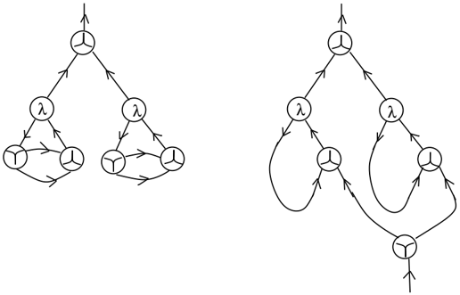
### Visual Description
## Flowchart Diagram: System Process Flow Comparison
### Overview
The image contains two side-by-side diagrams depicting node-based systems with directional flows. Both diagrams use circular nodes labeled with Greek letters (λ) and Latin letters (Y), connected by arrows indicating directional relationships. The left diagram shows a hierarchical structure, while the right introduces feedback loops.
### Components/Axes
- **Nodes**:
- Top node: Labeled "λ" (Greek lambda).
- Middle layer: Two nodes labeled "λ".
- Bottom layer: Four nodes labeled "Y" (Latin Y).
- **Arrows**:
- **Left Diagram**:
- Bidirectional arrows between the top "λ" and middle "λ" nodes.
- Unidirectional arrows from middle "λ" nodes to bottom "Y" nodes.
- Bidirectional arrows between the four bottom "Y" nodes.
- **Right Diagram**:
- Bidirectional arrows between the top "λ" and middle "λ" nodes.
- Unidirectional arrows from middle "λ" nodes to bottom "Y" nodes.
- Feedback loops from bottom "Y" nodes back to middle "λ" nodes.
- A final unidirectional arrow from the bottom-right "Y" node to a terminal node.
### Detailed Analysis
- **Left Diagram**:
- The top "λ" node distributes flow equally to two middle "λ" nodes via bidirectional arrows, suggesting mutual interaction or shared responsibility.
- Each middle "λ" node feeds into two bottom "Y" nodes via unidirectional arrows, indicating a one-way progression.
- The bottom "Y" nodes form a fully connected network via bidirectional arrows, implying reciprocal interactions or data exchange.
- **Right Diagram**:
- Similar hierarchical structure to the left diagram, but with added feedback loops from the bottom "Y" nodes to the middle "λ" nodes.
- The feedback loops suggest iterative processes or error correction mechanisms.
- A terminal node at the bottom-right "Y" node indicates a final output or endpoint.
### Key Observations
1. **Bidirectional vs. Unidirectional Flow**:
- The left diagram emphasizes mutual interactions at the bottom layer, while the right diagram introduces feedback to refine or adjust upstream processes.
2. **Terminal Node**:
- The right diagram’s terminal node implies a definitive endpoint, absent in the left diagram.
3. **Symmetry**:
- Both diagrams maintain symmetry in node distribution (1 top, 2 middle, 4 bottom nodes).
### Interpretation
- **System Behavior**:
- The left diagram likely represents a static, hierarchical system where processes flow downward without iteration.
- The right diagram models a dynamic system with feedback loops, enabling adaptation or correction based on downstream outputs.
- **Potential Applications**:
- The left diagram could represent a decision tree or linear workflow.
- The right diagram might model a control system, error-handling mechanism, or iterative algorithm (e.g., machine learning training loops).
- **Anomalies**:
- The terminal node in the right diagram breaks the symmetry of the left, suggesting a designed endpoint for specific outputs.
## Language Note
No non-English text is present. All labels use standard mathematical notation (Greek lambda, Latin Y).
</details>
Theorem 3.1 Let A ↦→ [ A ] be a transformation of a lambda term A into a graph [ A ] as described previously (multiple transformations are possible because of the choice of Υ trees). Then:
- (a) for any term A the graph [ A ] is in λGRAPH ,
- (b) if [ A ] ′ and [ A ]' are transformations of the term A then we may pass from [ A ] ′ to [ A ]' by using a finite number (exponential in the number of leaves of the syntactic tree of A ) of (CO-ASSOC) moves,
- (c) if B is obtained from A by α -conversion then we may pass from [ A ] to [ B ] by a finite sequence of (CO-ASSOC) moves,
- (d) let A,B ∈ T ( X ) be two terms and x ∈ X be a variable. Consider the terms λx.A and A [ x := B ] , where A [ x := B ] is the term obtained by substituting in A the free occurrences of x by B . We know that β reduction in lambda calculus consists in passing from ( λx.A ) B to A [ x := B ] . Then, by one β move in GRAPH applied to [( λx.A ) B ] we pass to a graph which can be further transformed into one of A [ x := B ] , via (global FAN-OUT) moves, (CO-ASSOC) moves and pruning moves,
- (e) with the notations from (d), consider the terms A and λx.Ax with x ∈ FV ( A ) ; then the η reduction, consisting in passing from λx.Ax to A , corresponds to the ext1 move applied to the graphs [ λx.Ax ] and [ A ] .
Proof. (a) we have to prove that for any node λ any oriented path in [ A ] starting at the left exiting edge of this node can be completed to a path which either terminates in a graph , or else terminates at the entry peg of this node, but this is clear. Indeed, either the bound variable (of this λ node in the syntactic tree of A ) is fresh, then the bound variable is replaced by a gate, or else, the bound variable is replaced by a tree of Υ gates. No matter which path we choose, we may complete it to a cycle passing by the said λ node.
(b) Clear also, because the (CO-ASSOC) move is designed for passing from a tree of Υ gates to another tree with the same number of leaves.
(c) Indeed, the names of bound variables of A do not affect the construction of [ A ], therefore if B is obtained by α -conversion of A , then [ B ] differs from [ A ] only by the particular choice of trees of Υ gates. But this is solved by (CO-ASSOC) moves.
(d) This is the surprising, maybe, part of the theorem. There are two cases: x is fresh for A or not. If x is fresh for A then in the graph [( λx.A ) B ] the name variable x is replaced by a gate. If not, then all the occurrences of x in A are connected by a Υ tree with root at the left peg of the λ gate where x appears as a bound variable.
In the case when x is not fresh for A , we see in the LHS of the figure the graph [( λx.A ) B ] (with a remanent decoration of 'x'). We perform a graphic ( β ) move and we obtain the graph from the right.
<details>
<summary>Image 28 Details</summary>
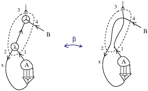
### Visual Description
## Diagram: Transformation Process Between States A and B
### Overview
The image depicts two interconnected diagrams labeled **A** and **B**, connected by a bidirectional arrow labeled **β**. Each diagram contains labeled components (1–4), a central node (λ), and a shared external element (x). The diagrams suggest a dynamic relationship or transformation process between states A and B.
---
### Components/Axes
- **Left Diagram (State A)**:
- **Components**:
- **A**: Central node with three downward arrows (possibly representing outputs or dependencies).
- **x**: External input/output at the bottom-left.
- **λ**: Central node with three outward arrows (labeled 1, 2, 3).
- **B**: External node connected to λ via arrow 4.
- **Labels**:
- Arrows: 1 (λ → A), 2 (x → λ), 3 (λ → x), 4 (λ → B).
- Nodes: A, B, λ, x.
- **Right Diagram (State B)**:
- **Components**:
- **A**: Central node with three downward arrows (similar to State A).
- **x**: External input/output at the bottom-left.
- **λ**: Central node with three outward arrows (labeled 1, 2, 3).
- **B**: External node connected to λ via arrow 4.
- **Labels**:
- Arrows: 1 (λ → A), 2 (x → λ), 3 (λ → x), 4 (λ → B).
- Nodes: A, B, λ, x.
- **Bidirectional Arrow (β)**: Connects the two diagrams, suggesting a reversible or iterative relationship between states A and B.
---
### Detailed Analysis
- **Left Diagram (State A)**:
- **Flow**:
1. **x** feeds into **λ** via arrow 2.
2. **λ** distributes outputs to **A** (arrow 1), **x** (arrow 3), and **B** (arrow 4).
3. **A** receives input from **λ** and generates three outputs (downward arrows).
- **Key Relationships**:
- **λ** acts as a hub, mediating interactions between **x**, **A**, and **B**.
- **B** is an external node dependent on **λ**.
- **Right Diagram (State B)**:
- **Flow**:
1. **x** feeds into **λ** via arrow 2.
2. **λ** distributes outputs to **A** (arrow 1), **x** (arrow 3), and **B** (arrow 4).
3. **A** receives input from **λ** and generates three outputs (downward arrows).
- **Key Relationships**:
- **λ** maintains the same role as in State A.
- **B** remains an external node dependent on **λ**.
- **Bidirectional Arrow (β)**:
- Indicates a transformation or equivalence between states A and B.
- Suggests the system can transition between these states while preserving core relationships (e.g., **λ** as a central mediator).
---
### Key Observations
1. **Symmetry**: Both diagrams share identical structural components (A, B, λ, x) and arrow labels (1–4), implying a consistent underlying mechanism.
2. **Central Node (λ)**: Acts as a critical mediator in both states, distributing inputs/outputs.
3. **External Node (B)**: Dependent on **λ** in both diagrams, suggesting it is an output or dependent variable.
4. **Bidirectional Relationship (β)**: Implies the system can evolve between states A and B without losing core functionality.
---
### Interpretation
The diagrams likely represent a **state transition** or **process equivalence** in a technical or mathematical system. The bidirectional arrow **β** suggests that states A and B are interchangeable or part of a cyclical process. The central node **λ** serves as a pivotal component, maintaining system integrity during transitions. The external node **B** and input **x** highlight dependencies on external factors, while the downward arrows from **A** may represent outputs or downstream effects. This structure could model concepts like **feedback loops**, **state machines**, or **equivalence classes** in engineering, computer science, or physics.
</details>
This graph can be transformed into a graph of A [ x := B ] via (global FAN-OUT) and (CO-ASSOC) moves. The case when x is fresh for A is figured next.
<details>
<summary>Image 29 Details</summary>
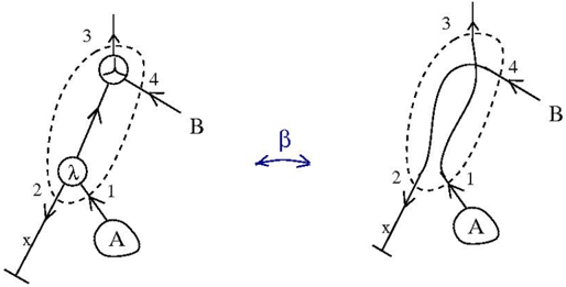
### Visual Description
## Diagram: Process Flow Transformation (A → B)
### Overview
The image depicts two interconnected diagrams labeled **A** and **B**, connected by a bidirectional arrow labeled **β**. Both diagrams feature numbered arrows (1–4), geometric shapes (dashed ovals, circles), and directional flows. The transformation **β** suggests a process or function mapping states between A and B.
### Components/Axes
- **Diagram A (Left)**:
- **Dashed Oval**: Encloses arrows 1, 2, 3, and 4.
- **Arrows**:
- **1**: Points to labeled region **A** (bottom-left).
- **2**: Points to labeled symbol **λ** (intermediate node).
- **3**: Vertical upward arrow (no explicit target).
- **4**: Points to labeled region **B** (top-right).
- **Labels**:
- **A**: Enclosed region (bottom-left).
- **λ**: Intermediate node (center-left).
- **B**: Enclosed region (top-right).
- **Diagram B (Right)**:
- **Dashed Oval**: Distorted compared to A, enclosing arrows 1, 2, 3, and 4.
- **Arrows**:
- **1**: Points to **A** (bottom-left).
- **2**: Points to **λ** (center-left).
- **3**: Curved upward arrow (no explicit target).
- **4**: Points to **B** (top-right).
- **Labels**:
- **A**: Enclosed region (bottom-left).
- **λ**: Intermediate node (center-left).
- **B**: Enclosed region (top-right).
- **Transformation β**:
- Bidirectional arrow between A and B, suggesting a reversible or iterative process.
### Detailed Analysis
- **Arrow Directions**:
- In both diagrams, arrows 1 and 2 consistently point to **A** and **λ**, respectively.
- Arrow 3 in Diagram A is vertical, while in Diagram B it curves upward, indicating a structural change in the process flow.
- Arrow 4 in both diagrams points to **B**, maintaining consistency in the final state.
- **Geometric Shapes**:
- The dashed ovals in A and B enclose the same set of arrows but differ in shape (circular vs. elongated), possibly representing different process boundaries or states.
- **Symbol λ**:
- Appears as an intermediate node in both diagrams, acting as a connector between **A** and **B**.
### Key Observations
1. **Structural Rearrangement**: The distortion of the dashed oval in Diagram B and the curved arrow 3 suggest a modification in the process flow or constraints.
2. **Consistency in Labels**: **A**, **λ**, and **B** remain constant across both diagrams, implying they are fixed states or regions.
3. **Bidirectional β**: The reversible arrow between A and B indicates the process can operate in both directions.
### Interpretation
The diagrams likely represent a **state transition system** or **process optimization scenario**:
- **A** and **B** could denote initial and final states, with **λ** as an intermediate step.
- The transformation **β** might symbolize a function (e.g., algorithm, physical process) that maps between these states.
- The structural differences between the diagrams (e.g., curved arrow 3, distorted oval) imply trade-offs or adjustments in the process efficiency or constraints.
- The bidirectional β suggests the system is reversible, allowing for feedback or iterative refinement.
This visualization emphasizes the relationship between components and the impact of process modifications on system behavior.
</details>
We see that the graph obtained by performing the graphic ( β ) move is the union of the graph of A and the graph of B with a gate added at the root. By pruning we are left with the graph of A , which is consistent to the fact that when x is fresh for A then ( λx.A ) B transforms by β reduction into A .
(e) In the next figure we see at the LHS the graph [ λx.Ax ] and at the RHS the graph [ A ].
<details>
<summary>Image 30 Details</summary>
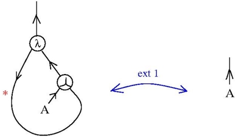
### Visual Description
## Diagram: System Component Flow with External Interaction
### Overview
The diagram illustrates a system with three primary components: a central node labeled "λ", a looped subsystem labeled "A", and an external interaction labeled "ext 1". Arrows indicate directional relationships, with a red asterisk marking a critical point in the subsystem.
### Components/Axes
1. **Central Node**:
- Labeled "λ" (Greek letter lambda)
- Positioned at the top-left with an upward-pointing arrow
2. **Looped Subsystem**:
- Labeled "A"
- Contains a circular path with a red asterisk (*) marking a critical node
- Contains an internal node with three outgoing arrows (trifurcation)
3. **External Interaction**:
- Labeled "ext 1"
- Represented by bidirectional curved arrows
- Connected to subsystem "A" via a vertical arrow labeled "A"
4. **Critical Marker**:
- Red asterisk (*) placed on the looped path of subsystem "A"
### Detailed Analysis
- **λ Node**: Acts as the primary input/output source, with a single upward arrow suggesting unidirectional flow.
- **Subsystem A**:
- Contains a closed loop with a critical point marked by the red asterisk
- Internal trifurcation node suggests branching logic or parallel processes
- **External Interaction (ext 1)**:
- Bidirectional arrows indicate two-way communication
- Vertical arrow labeled "A" suggests direct coupling between external system and subsystem A
### Key Observations
1. The red asterisk in subsystem A likely denotes a failure point, bottleneck, or special condition requiring attention
2. The trifurcation node within A suggests three possible processing paths or decision points
3. The vertical coupling between ext 1 and A implies direct influence on the subsystem's operation
4. The unidirectional flow from λ contrasts with the bidirectional ext 1 interaction
### Interpretation
This diagram appears to represent a control system or process flow with:
- A primary driver (λ) initiating operations
- A feedback loop (subsystem A) with inherent complexity (trifurcation) and a critical vulnerability (asterisk)
- External system interaction (ext 1) that can both influence and be influenced by the subsystem
The red asterisk's placement on the loop suggests this critical point may be essential for maintaining system stability or represents a point of potential failure. The bidirectional ext 1 interaction indicates the subsystem doesn't operate in isolation but engages in mutual exchange with external factors, potentially creating feedback loops that could amplify or mitigate the system's behavior.
</details>
The red asterisk marks the arrow which appears in the construction [ λx.Ax ] from the variable x , taking into account the hypothesis x ∈ FV ( A ). We have a pattern where we can apply the ext1 move and we obtain [ A ], as claimed.
As an example, let us manipulate the graph of Ω = ( λx. ( xx ))( λx. ( xx )):
<details>
<summary>Image 31 Details</summary>
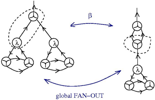
### Visual Description
## Diagram: Global FAN-OUT Process with Feedback Loop
### Overview
The diagram illustrates a two-stage process labeled "global FAN-OUT," showing the transformation and flow of entities between two hierarchical structures. Arrows labeled β indicate directional relationships, while dashed arrows suggest feedback mechanisms. The left structure has a feedback loop, while the right structure represents a streamlined output.
### Components/Axes
- **Nodes**:
- Left structure: Three nodes labeled λ (lambda), arranged in a triangular configuration with internal feedback loops.
- Right structure: Three nodes labeled λ (lambda) and one node labeled β (beta), arranged vertically with sequential connections.
- **Arrows**:
- Solid arrows labeled β connect the left and right structures.
- Dashed arrows form a feedback loop within the left structure.
- **Text**:
- "global FAN-OUT" at the bottom center.
- β (beta) between the two structures.
### Detailed Analysis
- **Left Structure**:
- Three λ nodes form a closed loop with bidirectional arrows, indicating mutual interactions or dependencies.
- Dashed arrows create a feedback loop, suggesting iterative refinement or error correction.
- **Right Structure**:
- Vertical arrangement of nodes implies a hierarchical or sequential process.
- The top λ node connects to two lower λ nodes via bidirectional arrows, while the bottom λ node connects to the β node via a unidirectional arrow.
- **β Arrows**:
- Represent transformation, transfer, or mapping between the two structures.
- The bidirectional β arrow implies a reversible or bidirectional relationship.
### Key Observations
1. The left structure emphasizes feedback and interdependence among λ nodes.
2. The right structure prioritizes linear flow, with β acting as a terminal or output node.
3. The global FAN-OUT label suggests scalability or distribution across multiple nodes.
4. The absence of numerical values indicates a conceptual or procedural model rather than quantitative data.
### Interpretation
This diagram likely represents a system architecture or workflow where:
- **Feedback loops** (left structure) enable adaptive or self-correcting behavior.
- **β transformations** mediate interactions between subsystems, possibly converting inputs (λ) into outputs.
- The **vertical right structure** may symbolize a simplified or optimized output after applying β.
- The "global FAN-OUT" terminology implies parallelism or distributed processing, with β serving as a central integration point.
The absence of numerical data limits quantitative analysis, but the emphasis on feedback and directional flow highlights the importance of iterative refinement and structured output in the system.
</details>
We can pass from the LHS figure to the RHS figure by using a graphic ( β ) move. Conversely, we can pass from the RHS figure to the LHS figure by using a (global FAN-OUT) move. These manipulations correspond to the well known fact that Ω is left unchanged after β reduction: let U = λx. ( xx ), then Ω = UU = ( λx. ( xx )) U ↔ UU = Ω.
## 3.1 Example: combinatory logic
S , K and I combinators in GRAPH . The combinators I = λx.x , K = λx. ( λy. ( xy )) and S = λx. ( λy. ( λz. (( xz )( yz )))) have the following correspondents in GRAPH , denoted by the same letters:
<details>
<summary>Image 32 Details</summary>
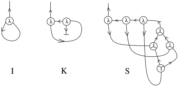
### Visual Description
## Diagram: Process Flow Representation
### Overview
The image contains three labeled diagrams (I, K, S) depicting abstract process flows. Each diagram uses nodes (circles) with lambda (λ) symbols and directional arrows to represent relationships or transitions. Diagram S is the most complex, featuring additional Y-shaped nodes and multiple interconnections.
### Components/Axes
- **Labels**:
- Diagram I: Single-node loop with a lambda (λ) symbol.
- Diagram K: Two-node loop with a lambda (λ) symbol and a downward arrow between nodes.
- Diagram S: Multi-node system with lambda (λ) and Y-shaped nodes, interconnected via arrows.
- **Arrows**:
- Solid arrows indicate directional flow.
- Dashed arrows (in Diagram K) suggest feedback or secondary pathways.
- **Y-shaped nodes**: Present only in Diagram S, possibly representing decision points or divergent states.
### Detailed Analysis
1. **Diagram I**:
- A single lambda (λ) node forms a closed loop with an upward arrow.
- No additional nodes or branches.
2. **Diagram K**:
- Two lambda (λ) nodes connected in a loop.
- A downward arrow between nodes implies a feedback mechanism or hierarchical relationship.
3. **Diagram S**:
- Three lambda (λ) nodes in a linear chain (top-to-bottom).
- Branching pathways connect to Y-shaped nodes, which further interconnect.
- Arrows form a network with no clear termination, suggesting cyclical or recursive processes.
### Key Observations
- **Progression**: Diagrams increase in complexity from I → K → S.
- **Feedback**: Diagram K introduces feedback loops absent in Diagram I.
- **Y-shaped nodes**: Unique to Diagram S, potentially indicating decision-making or state transitions.
- **Cyclicality**: All diagrams feature closed loops, emphasizing recurring processes.
### Interpretation
The diagrams likely represent stages of a system or process:
- **Diagram I**: A foundational, self-sustaining loop (e.g., basic feedback mechanism).
- **Diagram K**: Adds complexity via bidirectional interaction between components.
- **Diagram S**: Represents a highly interconnected system with multiple pathways and decision points (Y nodes), suggesting adaptability or branching logic.
The lambda (λ) symbols may denote variables, functions, or states, while arrows indicate causality or influence. The absence of termination points in Diagram S implies an open-ended or recursive system.
</details>
Proposition 3.2 (a) By one graphic ( β ) move I A transforms into A , for any A ∈ GRAPH with one output.
(b) By two graphic ( β ) moves, followed by a global pruning, for any A,B ∈ GRAPH with one output, the graph ( K A ) B transforms into A .
(c) By five graphic ( β ) moves, followed by one local pruning move, the graph ( S K ) K transforms into I .
(d) By three graphic ( β ) moves followed by a (global FAN-OUT) move, for any A,B,C ∈ GRAPH with one output, the graph (( S A ) B ) C transforms into the graph ( A C ) ( B C ) .
Proof. The proof of (b) is given in the next figure.
<details>
<summary>Image 33 Details</summary>
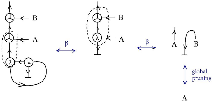
### Visual Description
## Diagram: System Interaction Flow with Global Pruning
### Overview
The diagram illustrates a three-stage system interaction process involving components labeled **A** and **B**, mediated by bidirectional relationships (β) and internal feedback loops (λ). The final stage introduces "global pruning" as a regulatory mechanism affecting the system's state.
---
### Components/Axes
1. **Stage 1 (Left Diagram)**:
- **A**: Central node with bidirectional arrows to **B** and internal feedback loops (λ).
- **B**: Connected to **A** via bidirectional arrows.
- **λ**: Self-loops on **A** and **B**, suggesting iterative processes or parameters.
- **β**: Arrows between diagrams indicate transitions between stages.
2. **Stage 2 (Middle Diagram)**:
- Simplified representation of **A** and **B** with dashed lines, implying abstraction or reduced complexity.
- **λ** remains as a self-loop on **A**.
3. **Stage 3 (Right Diagram)**:
- Minimalist depiction of **A** and **B** with a single bidirectional arrow (β).
- **Global pruning**: Vertical bidirectional arrows labeled "global pruning" between **A** and **B**, suggesting a system-wide optimization or constraint.
---
### Detailed Analysis
- **Stage 1**:
- **A** and **B** interact bidirectionally, with **A** having two feedback loops (λ). This suggests **A** undergoes iterative processing before influencing **B**.
- **B** receives input from **A** but lacks feedback loops, indicating a one-way dependency in this stage.
- **Stage 2**:
- Dashed lines between **A** and **B** imply a transitional or abstracted relationship. The removal of one **λ** loop on **B** may represent simplification or stabilization.
- **Stage 3**:
- The single bidirectional arrow (β) between **A** and **B** indicates a streamlined interaction.
- **Global pruning** introduces a regulatory layer, with arrows pointing both ways, suggesting mutual adjustment or balancing of **A** and **B** under external constraints.
---
### Key Observations
1. **Progressive Simplification**: The diagrams evolve from complex interactions (Stage 1) to abstracted (Stage 2) and minimalist (Stage 3) representations.
2. **Feedback Dynamics**: **λ** loops dominate **A**'s behavior, while **B** remains reactive until **global pruning** introduces bidirectional regulation.
3. **Pruning Mechanism**: "Global pruning" acts as a system-wide constraint, potentially optimizing or limiting interactions between **A** and **B**.
---
### Interpretation
This diagram likely models a computational or biological system where components **A** and **B** interact through iterative processes (λ) and transitional states (β). The introduction of "global pruning" in Stage 3 suggests a mechanism to prevent runaway feedback or stabilize the system. The progression from detailed to simplified diagrams may represent stages of system analysis, optimization, or abstraction. Notably, **A**'s self-loops (λ) imply it is a driver of internal dynamics, while **B**'s role shifts from reactive to regulated under pruning. The bidirectional β arrows emphasize mutual dependency, critical for maintaining system equilibrium.
</details>
The proof of (c) is given in the following figure.
(a) and (d) are left to the interested reader.
<details>
<summary>Image 34 Details</summary>
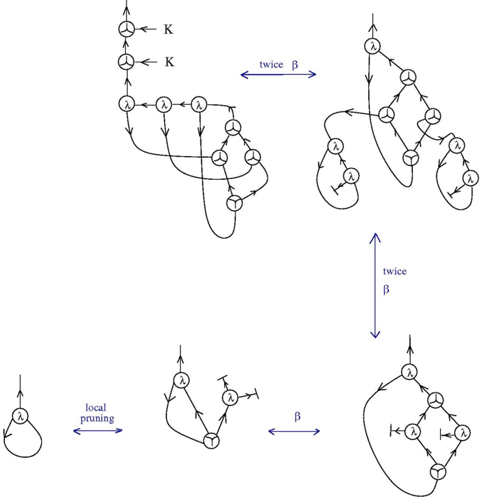
### Visual Description
## Flowchart Diagram: Process Transformation with Pruning
### Overview
The diagram illustrates a multi-stage process involving nodes labeled **X** and **K**, interconnected by directional arrows. Key operations include transformations labeled **β** and **twice β**, culminating in a "local pruning" step that simplifies the structure. The flow emphasizes iterative refinement and structural reduction.
---
### Components/Axes
1. **Nodes**:
- **X**: Represented as circles with internal arrows (e.g., `X → X` loops).
- **K**: Labeled nodes with bidirectional arrows (e.g., `K ↔ K`).
2. **Arrows**:
- **Directional**: Indicate unidirectional flow (e.g., `X → X`).
- **Bidirectional**: Denote feedback or mutual interaction (e.g., `K ↔ K`).
3. **Labels**:
- **β**: Arrows marked with "β" or "twice β" (e.g., `→ twice β →`).
- **Local Pruning**: A final step simplifying the structure (e.g., `→ local pruning →`).
---
### Detailed Analysis
1. **Top Section**:
- Three **K** nodes are vertically stacked, connected by bidirectional arrows (`K ↔ K`).
- A cluster of **X** nodes forms a loop with internal arrows (`X → X → X`).
- Arrows connect **K** and **X** nodes, suggesting interdependencies.
2. **Middle Section**:
- A transformation labeled **twice β** splits the flow into two paths:
- One path retains the original **X** cluster.
- The other path introduces a new **X** node with a loop (`X → X`).
3. **Bottom Section**:
- **Local Pruning** reduces complexity:
- Original **X** cluster collapses into a single node.
- Bidirectional arrows (`X ↔ X`) replace the loop, indicating simplified interactions.
---
### Key Observations
- **Complexity Reduction**: The process starts with a highly interconnected structure (top) and ends with a minimalized configuration (bottom).
- **Feedback Loops**: Bidirectional arrows (`K ↔ K`, `X ↔ X`) suggest iterative adjustments or mutual dependencies.
- **β Operations**: The "twice β" label implies repeated transformations, possibly scaling or amplifying effects.
---
### Interpretation
This diagram likely represents a **system optimization or data processing pipeline**:
1. **Initial State**: The top section depicts a complex, interdependent system (e.g., a network or algorithm).
2. **Transformation**: The **β** operations introduce controlled changes, possibly refining parameters or relationships.
3. **Pruning**: The final step eliminates redundancy, retaining only essential interactions (e.g., simplifying a model or workflow).
**Notable Patterns**:
- The bidirectional arrows in the pruned structure suggest a balance between efficiency and adaptability.
- The absence of numerical values implies a conceptual rather than quantitative analysis, focusing on structural relationships.
**Underlying Insight**:
The diagram emphasizes **iterative refinement**—starting with complexity, applying transformations, and ending with a streamlined system. This aligns with principles in machine learning (model pruning), systems engineering, or process optimization.
</details>
## 4 Using graphic lambda calculus
The manipulations of graphs presented in this section can be applied for graphs which represent lambda terms. However, they can also be applied for graphs which do not represent lambda terms.
Fixed points. Let's start with a graph A ∈ GRAPH , which has one distinguished input and one distinguished output.I represent this as follows.
$$\rightarrow A \rightarrow$$
For any graph B with one output, we denote by A ( B ) the graph obtained by grafting the output of B to the input of A .
I want to find B such that A ( B ) ↔ B , where ↔ means any finite sequence of moves in graphic lambda calculus. I call such a graph B a fixed point of A .
The solution of this problem is the same as in usual lambda calculus. We start from the following succession of moves:
<details>
<summary>Image 35 Details</summary>
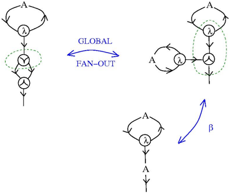
### Visual Description
## Diagram: System State Transitions and Global Fan-Out Process
### Overview
The diagram illustrates a multi-stage system with three primary components connected by labeled arrows. It depicts state transitions, global distribution mechanisms, and branching pathways. The system includes loops, conditional paths, and transformation processes.
### Components/Axes
1. **Left Structure**:
- Top loop labeled "A"
- Central node with "λ" (lambda)
- Two lower nodes:
- Left: "Y" (gamma)
- Right: "A"
- Dashed green oval encircling the lower nodes
- Vertical arrow exiting the bottom node
2. **Middle Structure**:
- Simple loop labeled "A"
- Central node with "λ"
- Direct connection to the right structure via "β" arrow
3. **Right Structure**:
- Top loop labeled "A"
- Central node with "λ"
- Lower node labeled "A" connected by dashed green line
- Dashed green oval encircling the entire structure
4. **Connecting Elements**:
- Blue bidirectional arrow between left and middle structures labeled "GLOBAL FAN-OUT"
- Blue arrow from middle to right structure labeled "β"
### Detailed Analysis
- **Left Structure**: Represents an initial state with a feedback loop ("A") and bifurcation into two paths ("Y" and "A"). The dashed oval suggests conditional processing of the lower nodes.
- **Middle Structure**: Simplified state with direct feedback loop, acting as an intermediary for global distribution.
- **Right Structure**: Final state with dual pathways - primary loop ("A") and optional secondary path ("A" via dashed line). The dashed oval indicates an alternative processing route.
- **Global Fan-Out**: Indicates bidirectional synchronization between initial and intermediary states.
- **β Transformation**: Represents a state transition or function application from intermediary to final state.
### Key Observations
1. The system exhibits hierarchical processing with three distinct stages
2. Dashed elements (oval boundaries and connecting lines) suggest optional/conditional operations
3. "Y" node introduces a unique pathway not present in other structures
4. "β" arrow implies irreversible transformation between states
5. All structures share identical "A" and "λ" labels, indicating conserved elements across states
### Interpretation
This diagram appears to model a computational or logical system with:
- **State Management**: The "λ" nodes likely represent state handlers or transformation functions
- **Control Flow**: The "A" loops suggest recurring processes or decision points
- **Global Coordination**: The "GLOBAL FAN-OUT" mechanism enables bidirectional communication between initial and intermediary states
- **Path Optimization**: The "β" transformation and dashed paths indicate potential optimization routes through the system
The presence of identical labels across structures suggests conserved elements in state transitions, while the unique "Y" node introduces system-specific processing. The bidirectional "GLOBAL FAN-OUT" implies a distributed architecture requiring synchronization between stages. The "β" transformation could represent a critical phase change or function application in the system's lifecycle.
</details>
This is very close to the solution, we only need a small modification:
<details>
<summary>Image 36 Details</summary>
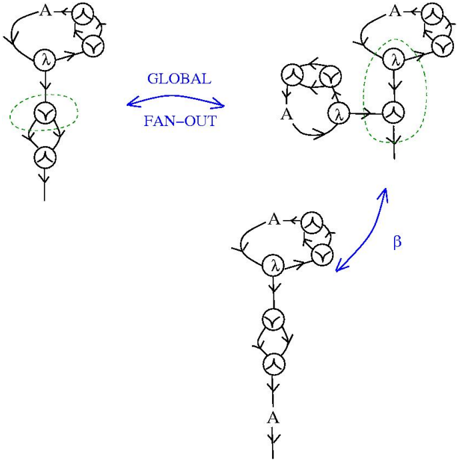
### Visual Description
## Diagram: System Flow with Global Fan-Out and Beta Transition
### Overview
The image depicts a three-part system flow diagram with labeled components and directional arrows. It illustrates transitions between states or processes, emphasizing a "GLOBAL FAN-OUT" mechanism and a "β" transition. The diagrams use standard flowchart notation with loops, arrows, and dashed circles to denote groupings or focus areas.
### Components/Axes
- **Left Diagram**:
- Contains a loop with nodes labeled **A**, **λ**, and **Y**.
- A dashed circle encloses **Y**, suggesting a subgroup or critical component.
- Arrows form a closed loop: **A → λ → Y → A**.
- **Middle Diagram (Global Fan-Out)**:
- Labeled **"GLOBAL FAN-OUT"** with bidirectional arrows.
- Contains nodes **A**, **λ**, and **Y** in a triangular configuration.
- Dashed circles enclose **A** and **Y**, indicating interconnected subgroups.
- Arrows show bidirectional flow between all nodes.
- **Right Diagram**:
- Contains a loop with nodes **A**, **λ**, and **Y**.
- A dashed circle encloses **A** and **Y**, similar to the middle diagram.
- An arrow labeled **β** connects this loop to the bottom diagram.
- **Bottom Diagram**:
- Linear flow with nodes **A**, **λ**, **Y**, and **A** in sequence.
- Arrows indicate unidirectional flow: **A → λ → Y → A**.
### Detailed Analysis
- **Labels**:
- **A**, **λ**, **Y**: Core nodes in all diagrams, likely representing states, processes, or entities.
- **GLOBAL FAN-OUT**: Indicates a distributed or parallelized transition between states.
- **β**: A directional transition between the middle and bottom diagrams.
- **Flow Direction**:
- Left diagram: Closed loop with emphasis on **Y** (dashed circle).
- Middle diagram: Bidirectional flow between all nodes, with **A** and **Y** highlighted.
- Right diagram: Closed loop with **A** and **Y** grouped.
- Bottom diagram: Linear progression ending in a self-loop at **A**.
### Key Observations
1. **Global Fan-Out**: The middle diagram suggests a decentralized or parallelized interaction between **A**, **λ**, and **Y**, with **A** and **Y** as focal points.
2. **β Transition**: The arrow labeled **β** implies a critical or probabilistic shift from the grouped **A/Y** loop to the linear **A→λ→Y→A** sequence.
3. **Dashed Circles**: Used to highlight subgroups (**Y** in the left diagram, **A/Y** in the middle and right diagrams), possibly denoting priority or interdependence.
### Interpretation
This diagram likely models a system with modular components (**A**, **λ**, **Y**) and dynamic interactions. The "GLOBAL FAN-OUT" mechanism may represent load balancing, parallel processing, or distributed state management. The **β** transition could signify a failure mode, optimization step, or probabilistic branching in the workflow.
- **Notable Patterns**:
- **A** appears as a central node in all diagrams, suggesting it is a primary actor or initiator.
- **Y** is consistently grouped (dashed circles), indicating its critical role in transitions.
- The linear bottom diagram contrasts with the bidirectional middle diagram, implying a shift from distributed to sequential processing.
- **Underlying Logic**:
- The use of loops and bidirectional arrows in the middle diagram contrasts with the unidirectional flow in the bottom diagram, hinting at adaptive system behavior.
- The **β** transition may represent a threshold or condition-triggered change in the system’s operational mode.
This structure could apply to computational workflows, network topologies, or process engineering systems where modularity and dynamic transitions are critical.
</details>
Grafting, application or abstraction? If the A , B from the previous paragraph were representing lambda terms, then the natural operation between them is not grafting, but the application. Or, in graphic lambda calculus the application it's represented by an elementary graph, therefore AB (seen as the term in lambda calculus which is obtained as the application of A to B ) is not represented as a grafting of the output of B to the input of A .
We can easily transform grafting into the application operation.
<details>
<summary>Image 37 Details</summary>
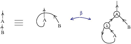
### Visual Description
## Diagram: Conceptual Relationship Model
### Overview
The image depicts a conceptual relationship model with two primary sections:
1. **Left Side**: A bidirectional equivalence between two vertical arrows labeled **A** (upward) and **B** (downward).
2. **Right Side**: A complex network of nodes (circles) and directional arrows, labeled **λ** and **β**, illustrating hierarchical or feedback relationships.
### Components/Axes
- **Left Section**:
- **Vertical Arrows**:
- **A**: Upward-pointing arrow labeled "A".
- **B**: Downward-pointing arrow labeled "B".
- **Equivalence Symbol**: Three horizontal lines (≡) connecting A and B, indicating bidirectional equivalence.
- **Right Section**:
- **Nodes**:
- **Upper Node**: Circle with a Y-shaped arrow pointing upward (no explicit label).
- **Lower Node**: Circle with a looped arrow labeled **λ**.
- **Arrows**:
- **β**: Double-headed blue arrow connecting the upper and lower nodes.
- **Directional Arrows**:
- Upper node → A and B (arrows point to labels A and B).
- Lower node → B and A (arrows point to labels B and A).
### Detailed Analysis
- **Left Section**:
- The equivalence (≡) suggests A and B are interchangeable or mutually dependent in this context.
- Spatial grounding: A is positioned above B, with the equivalence symbol centered between them.
- **Right Section**:
- **λ**: The looped arrow on the lower node implies a self-referential or cyclical process.
- **β**: The bidirectional arrow between nodes suggests a reversible or bidirectional interaction.
- **Flow**: Arrows from both nodes point to A and B, indicating these labels are outcomes or targets of the network.
### Key Observations
1. **Symmetry**: The left section’s equivalence mirrors the right section’s bidirectional β arrow.
2. **Cyclicality**: The λ loop on the lower node introduces a feedback mechanism absent in the left section.
3. **Hierarchy**: The upper node’s Y-shaped arrow may represent a bifurcation or decision point.
### Interpretation
This diagram likely models a system where:
- **A and B** are foundational elements (left section) that can exist in equilibrium.
- The **right section** expands this into a dynamic system with feedback (λ) and bidirectional interactions (β), where A and B are influenced by higher-order processes (upper node).
- The Y-shaped arrow on the upper node could symbolize a branching logic or probabilistic outcome, while the looped λ suggests iterative refinement or self-sustaining cycles.
The model may represent concepts in systems theory, control theory, or decision-making frameworks, where simple equivalences evolve into complex, interdependent structures.
</details>
Suppose that A and B are graphs representing lambda terms, more precisely suppose that A is representing a term (denoted by A too) and it's input represents a free variable x of the term A . Then the grafting of B to A is the term A [ x := B ] and the graph from the right is representing ( λx.A ) B , therefore both graphs are representing terms from lambda calculus.
We can transform grafting into something else:
<details>
<summary>Image 38 Details</summary>
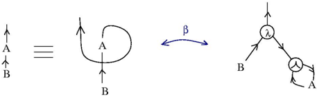
### Visual Description
## Diagram: Process Flow and Transformations
### Overview
The image consists of three interconnected diagrams illustrating relationships between elements labeled **A**, **B**, **λ**, and **β**. Arrows indicate directional flows, loops, and branching pathways.
### Components/Axes
1. **Left Diagram**:
- Vertical arrow labeled **A** (top) and **B** (bottom).
- Equivalence symbol (**≡**) connects the arrow to a looped arrow.
2. **Middle Diagram**:
- Looped arrow with bidirectional **β** (beta) annotation.
- Arrows labeled **A** (top) and **B** (bottom) form a closed loop.
3. **Right Diagram**:
- Branching structure with nodes labeled **λ** (lambda) and **β** (beta).
- Arrows labeled **A** (left) and **B** (right) diverge from **λ** and converge at **β**.
### Detailed Analysis
- **Left Diagram**:
- Represents a direct relationship between **A** and **B** (vertical flow).
- Equivalence to the looped arrow suggests cyclical or iterative behavior.
- **Middle Diagram**:
- **β** (beta) governs the loop, indicating a feedback mechanism.
- **A** and **B** are interdependent within the loop.
- **Right Diagram**:
- **λ** (lambda) acts as a decision node splitting into **A** and **B**.
- **β** (beta) integrates outputs from **A** and **B**, suggesting a synthesis or resolution step.
### Key Observations
- **Cyclicality**: The looped arrow (middle diagram) emphasizes recurring processes governed by **β**.
- **Branching Logic**: The right diagram’s structure implies conditional pathways (e.g., **A** vs. **B**) resolved by **β**.
- **Equivalence**: The left diagram’s equivalence symbol (**≡**) links linear and cyclical representations of **A** and **B**.
### Interpretation
The diagrams collectively model a system where:
1. **A** and **B** are foundational states or variables.
2. **β** (beta) regulates transitions between states (loop) and integrates outcomes (branching).
3. **λ** (lambda) introduces decision points, while **β** ensures convergence.
This could represent computational logic (e.g., state machines), biological pathways, or decision-making frameworks. The absence of numerical data suggests a focus on structural relationships rather than quantitative metrics.
</details>
This has no meaning in lambda calculus, but excepting the orientation of one of the arrows of the graph from the right, it looks like if the abstraction gate (the λ gate) plays the role of an application operation.
Zippers and combinators as half-zippers. Let's take n ≥ 1 a natural number and let's consider the following graph in GRAPH , called the n-zipper:
<details>
<summary>Image 39 Details</summary>
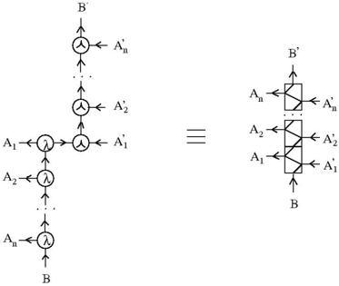
### Visual Description
## Diagram: Process Transformation Flowchart
### Overview
The image depicts two equivalent representations of a multi-stage transformation process. The left diagram shows a sequential flow of elements through transformation nodes, while the right diagram presents a consolidated block representation of the same process.
### Components/Axes
**Left Diagram:**
- **Nodes:**
- Input elements: `A₁, A₂, ..., Aₙ` (labeled sequentially from bottom to top)
- Transformation nodes: `λ` (lambda symbols) at each stage
- Output elements: `A'₁, A'₂, ..., A'ₙ` (transformed states of A₁ to Aₙ)
- Final output: `B'` (top node)
- **Arrows:**
- Vertical arrows connect `Aᵢ → λ → A'ᵢ` (transformation steps)
- Horizontal arrow connects `A'₁ → A'₂ → ... → A'ₙ → B'` (aggregation into final output)
**Right Diagram:**
- **Block Structure:**
- Input: `A₁, A₂, ..., Aₙ` (left side of block)
- Transformation: Diagonal arrows within a rectangular block labeled `B'`
- Output: `A'₁, A'₂, ..., A'ₙ` (right side of block)
- Final output: `B` (bottom node, equivalent to `B'` in left diagram)
**Shared Elements:**
- Lambda (`λ`) symbols denote transformation operations.
- Prime notation (`'`) indicates transformed states.
- Equivalence symbol (`≡`) links the two diagrams.
### Detailed Analysis
1. **Left Diagram Flow:**
- Each `Aᵢ` undergoes a transformation via `λ` to produce `A'ᵢ`.
- Transformed elements (`A'₁` to `A'ₙ`) are sequentially aggregated into `B'`.
- Vertical stacking implies hierarchical or sequential dependency.
2. **Right Diagram Structure:**
- The block represents a matrix-like transformation where inputs `Aᵢ` are mapped to outputs `A'ᵢ` via `B'`.
- Diagonal arrows suggest linear or direct mapping between input and output states.
- `B` at the bottom of the right diagram is equivalent to `B'` in the left diagram.
3. **Equivalence (`≡`):**
- The two diagrams represent the same process:
- Left: Stepwise transformation and aggregation.
- Right: Compact block representation of the same transformation.
### Key Observations
- **Consistency of Transformation:** The lambda (`λ`) symbols are identical in both diagrams, confirming the same operation is applied at each stage.
- **Prime Notation:** `A'ᵢ` and `B'` denote transformed states, while `B` (right diagram) is functionally equivalent to `B'`.
- **Dimensionality:** The left diagram emphasizes sequential processing, while the right diagram abstracts the process into a single block, suggesting a linear algebra or matrix-based interpretation.
### Interpretation
This diagram illustrates a **linear transformation pipeline** where:
1. Input elements (`Aᵢ`) are individually transformed via a function `λ` into intermediate states (`A'ᵢ`).
2. The transformed states are then combined (via aggregation or summation) into a final output (`B'` or `B`).
3. The equivalence (`≡`) implies that the stepwise process (left) and the block representation (right) are mathematically or computationally equivalent, likely representing a matrix operation or a linear system.
**Notable Patterns:**
- The use of primes (`'`) and lambda (`λ`) suggests a formal mathematical framework, possibly in linear algebra, signal processing, or control theory.
- The right diagram’s block structure hints at a matrix representation, where `B'` acts as a transformation matrix mapping `Aᵢ` to `A'ᵢ`.
**Underlying Assumptions:**
- The process is linear and reversible (implied by the equivalence symbol).
- The transformation `λ` is consistent across all `Aᵢ` elements.
- The final output (`B'`/`B`) depends on the cumulative effect of all transformed `A'ᵢ` elements.
</details>
At the left is the n-zipper graph; at the right is a notation for it, or a 'macro'. The zipper graph is interesting because it allows to perform (nontrivial) graphic beta moves in a fixed order. In the following picture is figured in red the place where the first graphic beta move is applied.
<details>
<summary>Image 40 Details</summary>
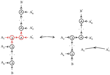
### Visual Description
## Diagram: System Transformation Flowchart
### Overview
The image depicts a two-part diagram connected by a bidirectional arrow, illustrating a transformation process between two system states. The left diagram shows a complex network with feedback loops, while the right diagram presents a simplified linear structure.
### Components/Axes
**Left Diagram (Input State):**
- **Nodes:**
- `A₁`, `A₂`, ..., `Aₙ` (input nodes, labeled sequentially)
- `B` (central node)
- `B'` (output node)
- **Connections:**
- Red arrows indicate feedback loops:
- `A₁ ↔ A₁'`
- `A₂ ↔ A₂'`
- `B ↔ B'`
- Black arrows show unidirectional flow:
- `A₁ → A₂ → ... → Aₙ → B`
- **Highlight:** A red circle emphasizes the `A₁ ↔ A₁'` feedback loop.
**Right Diagram (Output State):**
- **Nodes:**
- `A₁'`, `A₂'`, ..., `Aₙ'` (transformed input nodes)
- `B'` (output node)
- **Connections:**
- Black arrows show a linear chain:
- `A₁' → A₂' → ... → Aₙ' → B'`
**Connecting Arrow:**
- A bidirectional arrow links the two diagrams, suggesting a reversible transformation.
### Detailed Analysis
1. **Left Diagram Structure:**
- The input state (`A₁` to `Aₙ`) feeds into `B`, which outputs to `B'`.
- Feedback loops (`A₁ ↔ A₁'`, `A₂ ↔ A₂'`, `B ↔ B'`) imply iterative adjustments or error correction.
- The red circle around `A₁ ↔ A₁'` suggests this loop is a focal point for analysis.
2. **Right Diagram Structure:**
- The output state (`A₁'` to `Aₙ'`) flows linearly into `B'`, with no feedback.
- Simplification from the left diagram’s complexity indicates a streamlined process.
3. **Bidirectional Arrow:**
- Implies the transformation between states is reversible, though the right diagram’s lack of feedback loops may limit reversibility in practice.
### Key Observations
- **Feedback Dominance:** The left diagram’s feedback loops (highlighted in red) contrast with the right diagram’s linearity, suggesting feedback is critical in the input state but absent in the output.
- **Node Reduction:** The right diagram omits `B` and `B'`, focusing only on transformed `A'` nodes and `B'`.
- **Unidirectional Flow:** The right diagram’s black arrows enforce a strict sequence, unlike the left diagram’s bidirectional feedback.
### Interpretation
This diagram likely represents a system optimization or abstraction process:
1. **Input State (Left):** A complex, feedback-driven system where components (`A₁`–`Aₙ`, `B`) interact iteratively to produce `B'`.
2. **Output State (Right):** A simplified, linearized version of the system, possibly after optimization or error correction. The removal of feedback loops (`A₁'`–`Aₙ'` to `B'`) suggests a focus on efficiency or stability.
3. **Bidirectional Arrow:** While the transformation is theoretically reversible, the right diagram’s lack of feedback may make practical reversibility challenging.
The red circle around `A₁ ↔ A₁'` highlights a critical interaction point, possibly indicating a bottleneck or key variable in the system’s behavior. The absence of numerical data prevents quantitative analysis, but the structural contrast emphasizes trade-offs between complexity and simplicity in system design.
</details>
In terms of zipper notation this graphic beta move has the following appearance:
<details>
<summary>Image 41 Details</summary>
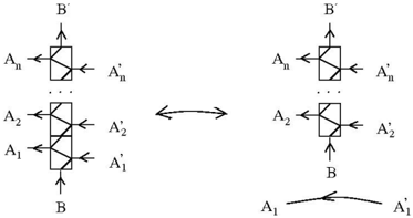
### Visual Description
## Diagram: Transformation of Layered System Components
### Overview
The image depicts two interconnected diagrams representing a layered system transformation. The left diagram shows a vertical stack of components (A₁, A₂, ..., Aₙ) with bidirectional arrows to their primed counterparts (A'₁, A'₂, ..., A'_ₙ), while the right diagram simplifies the structure by connecting A₁ directly to A'₁ via a curved arrow. Both diagrams include a terminal component labeled "B" at the base.
### Components/Axes
- **Left Diagram**:
- **Vertical Stack**: Labeled A₁ (bottom), A₂, ..., Aₙ (top).
- **Bidirectional Arrows**: Connect each Aᵢ to A'_ᵢ (e.g., A₁ ↔ A'₁, A₂ ↔ A'₂).
- **Terminal Node**: Labeled "B" at the bottom.
- **Right Diagram**:
- **Simplified Stack**: Same Aᵢ and A'_ᵢ labels but only A₁ ↔ A'₁ is explicitly shown with a curved arrow.
- **Terminal Node**: Labeled "B" at the bottom.
- **Bidirectional Arrow**: Connects the left and right diagrams, suggesting equivalence or transformation.
### Detailed Analysis
- **Left Diagram**:
- Each Aᵢ component has a straight bidirectional arrow to A'_ᵢ, implying direct, linear relationships or transformations.
- The vertical stacking suggests hierarchical or sequential dependencies.
- **Right Diagram**:
- The curved arrow between A₁ and A'₁ may indicate a non-linear, indirect, or more complex relationship compared to the left diagram.
- The absence of intermediate A₂–Aₙ components in the right diagram implies simplification or abstraction.
### Key Observations
1. **Bidirectional Relationships**: All Aᵢ ↔ A'_ᵢ connections are reversible, suggesting symmetry in the system's behavior.
2. **Hierarchical Structure**: The left diagram emphasizes layered dependencies, while the right diagram abstracts this into a single direct relationship.
3. **Curved Arrow Significance**: The curved arrow in the right diagram could represent a feedback loop, non-linear process, or emergent property not present in the left diagram.
### Interpretation
The diagrams likely illustrate a **system transformation** where:
- The left diagram represents a detailed, step-by-step process (e.g., data flow through layers A₁–Aₙ to produce A'₁–A'_ₙ, with B as an output or boundary condition).
- The right diagram abstracts this into a simplified model, where A₁ directly influences A'₁, possibly representing a higher-level equivalence or emergent behavior.
- The bidirectional arrows suggest the system is **reversible** or **symmetric**, allowing transformations in both directions.
- The terminal "B" component may act as a **boundary condition**, **output**, or **reference point** for the system.
### Notable Patterns
- The left diagram’s vertical stacking implies **cumulative or sequential processing**, while the right diagram’s simplification suggests **optimization** or **model reduction**.
- The curved arrow in the right diagram introduces ambiguity about the nature of the A₁–A'₁ relationship, requiring further context to determine if it represents a delay, feedback, or non-linear interaction.
### Conclusion
This diagram highlights the trade-off between **detailed modeling** (left) and **abstraction** (right), with the bidirectional arrow emphasizing the system’s flexibility. The curved arrow in the right diagram invites further investigation into the nature of the A₁–A'₁ relationship, potentially uncovering hidden dynamics in the system.
</details>
We see that a n-zipper transforms into a (n-1)-zipper plus an arrow. We may repeat this move, as long as we can. This procedure defines a 'zipper move':
<details>
<summary>Image 42 Details</summary>
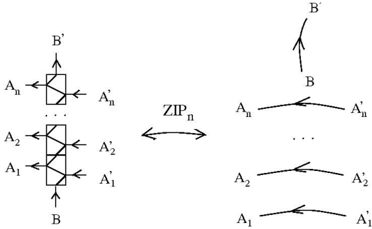
### Visual Description
## Diagram: Centralized vs. Distributed System Interaction
### Overview
The diagram illustrates a comparison between a centralized system (left) and a distributed system (right), connected via a bidirectional "ZIP_n" mechanism. Arrows indicate data flow, feedback loops, and transformations between components labeled A_n, A'_n, B, and B'.
### Components/Axes
- **Left Side (Centralized System)**:
- **Block**: Contains nested arrows between A_n → A'_n and B → B', suggesting sequential processing or transformation.
- **Labels**: A_n, A'_n, B, B' with vertical alignment.
- **Right Side (Distributed System)**:
- **Individual Arrows**: Direct connections between A_n → A'_n, A_2 → A'_2, A_1 → A'_1, and B → B', indicating parallel or decentralized operations.
- **Curved Arrows**: Feedback loops from B' to B and A'_n to A_n, implying iterative adjustments or error correction.
- **ZIP_n**: A bidirectional arrow between the two systems, symbolizing synchronization, data exchange, or protocol bridging.
### Detailed Analysis
- **Centralized System**:
- A_n and B are input nodes feeding into a single processing block.
- Outputs A'_n and B' are generated after transformation within the block.
- Vertical stacking of A_1, A_2, ..., A_n suggests hierarchical or layered processing.
- **Distributed System**:
- Each A_i and B operates independently, with direct transformations to A'_i and B'.
- Feedback loops (B' → B, A'_n → A_n) indicate dynamic recalibration or validation.
- **ZIP_n**:
- Positioned centrally, acting as a bridge between centralized and distributed components.
- Bidirectional flow implies mutual dependency or real-time coordination.
### Key Observations
1. **Centralization vs. Distribution**: The left side represents a monolithic architecture, while the right side depicts modular, parallel processing.
2. **Feedback Mechanisms**: Both systems incorporate feedback, but the distributed system emphasizes localized adjustments (e.g., A'_n → A_n).
3. **ZIP_n Role**: Likely a protocol or middleware enabling interoperability between centralized and distributed components.
### Interpretation
The diagram highlights a hybrid architecture where a centralized system (e.g., a server) interacts with distributed nodes (e.g., clients or edge devices) via a synchronization protocol (ZIP_n). Feedback loops suggest adaptive behavior, such as error correction or load balancing. The bidirectional ZIP_n flow implies that both systems influence each other, possibly for data consistency or resource optimization. This could model scenarios like cloud-edge computing, distributed databases, or IoT networks with centralized management.
</details>
We may see the 1-zipper move as the graphic beta move, which transforms the 1-zipper into two arrows.
The combinator I = λx.x satisfies the relation IA = A . In the next figure it is shown that I (figured in green), when applied to A , is just a half of the 1-zipper, with an arrow added (figured in blue).
<details>
<summary>Image 43 Details</summary>
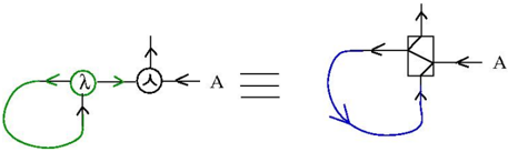
### Visual Description
## Diagram: Equivalence of Two System Representations
### Overview
The image depicts two equivalent diagrams connected by the equivalence symbol (≡). The left diagram uses green and black elements, while the right uses blue and black. Both diagrams include directional arrows and symbolic components, suggesting a flow or process leading to a shared endpoint labeled "A".
### Components/Axes
- **Left Diagram**:
- **Green Loop**: A closed loop with a lambda symbol (λ) inside.
- **Black Circle**: Contains a triangle symbol (△) and is connected to the green loop.
- **Node "A"**: Final endpoint for both diagrams.
- **Right Diagram**:
- **Blue Loop**: A closed loop with a square containing a triangle (△) inside.
- **Node "A"**: Final endpoint, identical to the left diagram.
- **Equivalence Symbol (≡)**: Connects the two diagrams, indicating they represent the same system or concept.
### Detailed Analysis
- **Left Diagram Flow**:
1. The green loop (λ) feeds into the black circle (△).
2. The black circle directs output to node "A".
- **Right Diagram Flow**:
1. The blue loop (△ inside a square) feeds into node "A".
- **Symbolic Relationships**:
- The lambda (λ) in the left diagram may represent a variable, function, or parameter.
- The triangle (△) in both diagrams could symbolize a transformation, operation, or state.
- The square enclosing the triangle in the right diagram might denote a constrained or modified version of the triangle’s function.
### Key Observations
1. **Equivalence**: The diagrams are structurally distinct but functionally equivalent, as denoted by ≡.
2. **Color Coding**:
- Green (left) and blue (right) loops differentiate the two representations.
- Black elements (triangle, node "A") are consistent across both diagrams.
3. **Directionality**: All arrows point toward node "A", emphasizing it as the terminal state or output.
### Interpretation
The diagrams likely represent two equivalent mathematical, computational, or logical systems. The left diagram’s use of λ and △ suggests a parameter-driven process, while the right diagram’s square-with-triangle may indicate a structured or constrained version of the same process. The equivalence implies that despite differences in representation (e.g., symbolic vs. geometric), both systems achieve the same outcome at node "A". This could reflect principles in fields like category theory, computer science (e.g., equivalent code paths), or physics (e.g., equivalent force diagrams).
No numerical data or trends are present; the focus is on symbolic and structural equivalence.
</details>
By opening the zipper we obtain A , as it should.
The combinator K = λxy.x satisfies KAB = ( KA ) B = A . In the next figure the combinator K (in green) appears as half of the 2-zipper, with one arrow and one termination gate added (in blue).
<details>
<summary>Image 44 Details</summary>
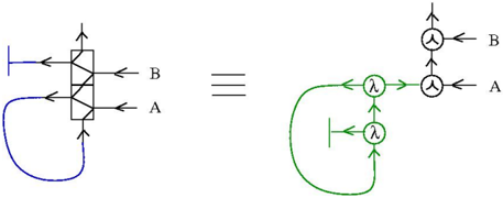
### Visual Description
## Diagram: Equivalent System Representation
### Overview
The image depicts two equivalent system diagrams connected by a triple-bar equivalence symbol (≡). The left diagram uses a blue square with internal arrows, while the right diagram uses green circular nodes with lambda (λ) symbols. Both diagrams include labeled inputs/outputs (A, B) and directional flow indicators.
### Components/Axes
- **Left Diagram (Blue Square)**:
- Central square with diagonal internal arrows (no explicit labels).
- Arrows labeled **A** (input) and **B** (output) on the left and top sides, respectively.
- Feedback loop arrow at the bottom (no label).
- **Right Diagram (Green Nodes)**:
- Two green circular nodes labeled **λ** (lambda symbols).
- Arrows connecting nodes in a loop (clockwise).
- Arrows labeled **A** (input) and **B** (output) on the left and top sides, respectively.
- **Equivalence Symbol**:
- Triple-bar symbol (≡) between diagrams, indicating functional equivalence.
### Detailed Analysis
- **Left Diagram**:
- The square’s internal arrows suggest a bidirectional or cross-coupled process.
- Input **A** enters the system, processes through the square, and exits as output **B**.
- Feedback loop implies self-reinforcement or recycling of output.
- **Right Diagram**:
- Two lambda nodes form a closed loop, suggesting iterative or cyclical processing.
- Input **A** enters the loop, processes through both λ nodes, and exits as output **B**.
- Lambda symbols may represent parameters, feedback factors, or transformation steps.
### Key Observations
1. **Equivalence**: Both diagrams represent the same system behavior despite differing visual structures.
2. **Feedback Mechanisms**: Both systems incorporate feedback (left: explicit loop; right: implicit loop via λ nodes).
3. **Input/Output Symmetry**: Input **A** and output **B** are positioned identically in both diagrams.
### Interpretation
The diagram illustrates two equivalent representations of a dynamic system:
- The **left diagram** emphasizes structural simplicity (a single processing unit with feedback).
- The **right diagram** highlights modularity (two interconnected processing steps with cyclical behavior).
- The lambda (λ) symbols likely denote adjustable parameters or feedback coefficients, critical for system tuning.
- The equivalence (≡) implies that both models can be used interchangeably for analysis, depending on the required level of detail.
This representation is common in control systems, signal processing, or feedback loop analysis, where multiple equivalent models aid in optimization or fault diagnosis.
</details>
After opening the zipper we obtain a pair made by A and B which gets the termination gate on top of it. A global pruning move sends B to the trash bin.
Finally, the combinator S = λxyz. (( xz )( yz )) satisfies SABC = (( SA ) B ) C = ( AC )( BC ). The combinator S (in green) appears to be made by half of the 3-zipper, with some arrows and also with a 'diamond' added (all in blue). Interestingly, the diamond looks alike the ones from the emergent algebra sector, definition 5.4.
Expressed with the help of zippers, the relation SKK = I appears like this.
<details>
<summary>Image 45 Details</summary>
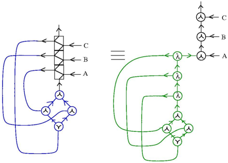
### Visual Description
## Diagram: Process Flow Equivalence
### Overview
The image presents two interconnected diagrams (blue on the left, green on the right) linked by an equivalence symbol (≡). Both diagrams use arrows, labeled nodes, and symbolic elements to represent processes or relationships.
### Components/Axes
- **Left Diagram (Blue)**:
- **Top Box**: A labeled box with internal grid lines, connected to three arrows labeled **A**, **B**, and **C** pointing outward.
- **Lower Nodes**: Three interconnected circles with triangle symbols (▲) and one circle with a **Y** symbol. Arrows form a loop between these nodes.
- **Flow**: Arrows from the box point to the lower nodes, and internal arrows create a feedback loop.
- **Right Diagram (Green)**:
- **Vertical Stack**: Three circles labeled **C**, **B**, and **A** (top to bottom), connected by upward-pointing arrows.
- **Lower Loop**: A cluster of circles with lambda symbols (λ) and **Y** symbols, connected by arrows forming a closed loop.
- **Flow**: Arrows from the vertical stack point to the lower loop, with internal arrows creating a feedback cycle.
- **Equivalence Symbol**: A horizontal ≡ symbol connects the two diagrams, suggesting they represent equivalent processes.
### Detailed Analysis
- **Left Diagram**:
- The box (A, B, C) likely represents a decision or input stage, with arrows directing flow to the lower nodes.
- The lower nodes (▲, Y) may symbolize intermediate states or operations, with the loop indicating cyclical processing.
- **Right Diagram**:
- The vertical stack (C → B → A) suggests a hierarchical or sequential process, with arrows pointing upward.
- The lower loop (λ, Y) mirrors the left diagram’s feedback structure, implying equivalence in operational logic.
### Key Observations
1. **Symbolic Consistency**: Both diagrams use **Y** symbols and loops, suggesting shared functional roles.
2. **Directional Flow**: Arrows in both diagrams point toward the lower nodes, emphasizing a bottom-up or cyclical process.
3. **Equivalence**: The ≡ symbol implies the diagrams are interchangeable representations of the same system.
### Interpretation
The diagrams likely model a process where inputs (A, B, C) are processed through intermediate states (▲, λ, Y) with feedback loops. The left diagram’s box may represent a centralized control or input hub, while the right diagram’s vertical stack suggests a hierarchical structure. The equivalence symbol indicates that despite differences in visual representation, both diagrams describe the same underlying logic. The use of **Y** and looped arrows emphasizes iterative or recursive operations, possibly in computational or decision-making contexts.
</details>
Lists and currying. With the help of zippers, we may enhance the procedure of turning grafting into the application operation. We have a graph A ∈ GRAPH which has one output and several inputs.
<details>
<summary>Image 46 Details</summary>
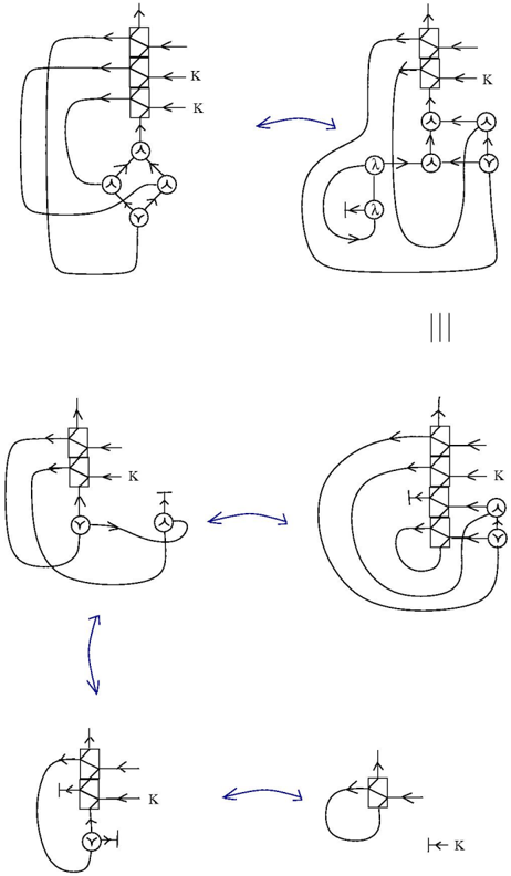
### Visual Description
## Flowchart Diagram: Process Flow with Transformations
### Overview
The image depicts a multi-stage flowchart with interconnected components and directional arrows. It consists of three primary diagrams (labeled I, II, III) connected by blue arrows indicating transformations or sequential steps. Each diagram contains geometric shapes (rectangles, circles) labeled with symbols (K, Y, λ) and directional arrows showing data or process flow.
### Components/Axes
- **Symbols**:
- **K**: Rectangle with diagonal crosshatch (appears in all diagrams, positioned at the top).
- **Y**: Circle with checkmark (appears in all diagrams, positioned at the bottom).
- **λ**: Circle with horizontal line (appears in diagrams II and III, positioned in the middle).
- **Arrows**:
- **Black arrows**: Indicate primary flow direction within each diagram.
- **Blue arrows**: Connect diagrams I → II → III, suggesting sequential transformations.
- **Labels**:
- Vertical line labeled "III" separates diagrams II and III.
- No explicit axis titles or numerical scales present.
### Detailed Analysis
1. **Diagram I**:
- **Structure**:
- K (top) → Y (bottom) via two parallel black arrows.
- Y connects to three λ nodes via bidirectional arrows.
- λ nodes form a triangular feedback loop.
- **Flow**: Input (K) splits into two paths to Y, which then distributes to λ nodes in a cyclic manner.
2. **Diagram II**:
- **Structure**:
- K (top) → Y (bottom) via a single black arrow.
- Y connects to λ via a bidirectional arrow.
- λ loops back to K via a blue arrow.
- **Flow**: Linear path from K to Y, with λ acting as a feedback mechanism to K.
3. **Diagram III**:
- **Structure**:
- K (top) → Y (bottom) via a single black arrow.
- Y connects to λ via a unidirectional arrow.
- λ loops back to K via a black arrow.
- **Flow**: Simplified feedback loop compared to Diagram II, with λ directly returning to K.
### Key Observations
- **Consistency**: K and Y are constant across all diagrams, suggesting they represent fixed input/output nodes.
- **Feedback Complexity**: Diagrams I and II show increasingly complex feedback loops involving λ, while Diagram III simplifies the loop.
- **Blue Arrows**: Indicate transformations between diagrams, possibly representing iterative refinement or process evolution.
- **Symbol Roles**:
- **K**: Likely a "key" or "control" component (rectangle with crosshatch).
- **Y**: Likely a "yes" or "output" node (checkmark symbol).
- **λ**: Likely a "lambda" transformation or intermediate step (horizontal line).
### Interpretation
The flowchart illustrates a multi-stage process with iterative feedback and transformation steps. Diagram I represents the most complex system, with distributed feedback among λ nodes. Diagrams II and III simplify the feedback mechanism, suggesting optimization or reduction in complexity. The blue arrows imply that each subsequent diagram (I→II→III) represents a refined or evolved version of the process. The use of K (control), Y (output), and λ (transformation) aligns with common technical notation for system diagrams, where feedback loops are critical for stability or adaptation. The absence of numerical data suggests this is a conceptual model rather than a quantitative analysis.
</details>
<details>
<summary>Image 47 Details</summary>
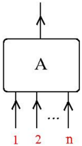
### Visual Description
## Diagram: Central Component "A" with Sequential Arrows
### Overview
The image depicts a rectangular block labeled "A" at the center, with multiple upward-pointing arrows extending from its base. Each arrow is sequentially labeled with red text: "1", "2", ..., "n". The arrows are evenly spaced and aligned vertically beneath the rectangle.
### Components/Axes
- **Central Block**: A horizontally oriented rectangle labeled "A" in bold black text at its center.
- **Arrows**:
- Multiple vertical arrows originate from the bottom edge of the rectangle.
- Each arrow is labeled with a red integer: "1", "2", ..., "n" (where "n" represents an unspecified upper limit).
- Arrows are evenly spaced and aligned in a single column beneath the rectangle.
### Detailed Analysis
- **Labels**:
- The central block is explicitly labeled "A".
- Arrows are labeled with sequential integers starting at "1" and ending at "n", suggesting a countable or iterative process.
- **Spatial Relationships**:
- Arrows are positioned directly below the rectangle, maintaining vertical alignment.
- The sequence "1, 2, ..., n" implies a progression or hierarchy, though the exact nature (e.g., steps, inputs, outputs) is unspecified.
### Key Observations
- The diagram lacks numerical data, trends, or explicit contextual labels beyond "A" and the sequential integers.
- The upward direction of the arrows may imply flow, directionality, or dependency (e.g., inputs to "A", outputs from "A", or stages in a process).
- The use of "n" indicates a variable or scalable system, but no specific value is provided.
### Interpretation
This diagram likely represents a conceptual or abstract system where:
1. **Component "A"** serves as a central node or process.
2. The **sequential arrows (1 to n)** could symbolize:
- Inputs or resources fed into "A".
- Outputs or stages generated by "A".
- Iterative steps in a workflow or algorithm.
3. The absence of additional context (e.g., labels, units, or annotations) suggests the diagram is intentionally minimalist, focusing on structural relationships rather than quantitative details.
The upward direction of the arrows might imply causality, progression, or dependency, but without further context, this remains speculative. The diagram could apply to fields like systems engineering, data flow diagrams, or process modeling, where "A" acts as a hub and the arrows represent connected elements.
</details>
We use an n-zipper in order to clip the inputs with the output.
<details>
<summary>Image 48 Details</summary>
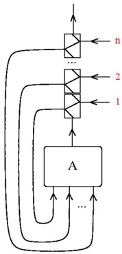
### Visual Description
## Flowchart Diagram: Central Process "A" with Multi-Stage Feedback Loop
### Overview
The diagram depicts a hierarchical system with a central processing unit labeled "A" receiving inputs from multiple stages (labeled 1, 2, n) and providing feedback to those stages. The structure suggests an iterative or cyclical process with decision points represented by triangular shapes.
### Components/Axes
- **Central Box**: Labeled "A" (likely represents a core system/process)
- **Input Arrows**:
- Three upward-pointing arrows labeled "1", "2", and "n" (indicating sequential or variable stages)
- Arrows originate from triangular shapes (possibly decision nodes)
- **Feedback Arrows**:
- Three downward-pointing arrows from "A" looping back to the lower stages
- **Triangular Shapes**:
- Positioned between input arrows and "A"
- Labeled with numbers matching the input arrows (1, 2, n)
- **Loop Structure**:
- Arrows form closed loops between "A" and stages 1-2-n
### Detailed Analysis
1. **Stage Progression**:
- Input stages (1 → 2 → n) feed into triangular decision nodes
- Triangular nodes direct flow toward central process "A"
- "n" suggests variable or scalable stages beyond fixed levels 1-2
2. **Feedback Mechanism**:
- "A" outputs three feedback arrows returning to stages 1-2-n
- Creates closed-loop system where outputs influence earlier stages
3. **Topological Features**:
- Central "A" acts as convergence point for all input stages
- Triangular shapes positioned at midpoints between stages and "A"
- Arrows maintain consistent directionality (upward for inputs, downward for feedback)
### Key Observations
- **Hierarchical Relationships**:
- Stages 1-2-n form a linear progression feeding into "A"
- Feedback arrows create bidirectional relationships between "A" and all stages
- **Scalability**:
- Use of "n" implies system can accommodate additional stages beyond shown levels
- **Decision Points**:
- Triangular shapes likely represent conditional processing or filtering steps
### Interpretation
This diagram represents a **cyclical processing system** where:
1. Input data flows through multiple processing stages (1 → 2 → n)
2. Each stage includes decision-making components (triangular nodes)
3. Central process "A" integrates inputs from all stages
4. System maintains continuous operation through feedback loops
The architecture suggests applications in:
- Machine learning pipelines with iterative refinement
- Industrial control systems with multi-stage processing
- Data transformation workflows requiring feedback correction
- Recursive algorithms with variable iteration counts
The use of "n" indicates the system's adaptability to different scales, while the triangular decision nodes imply conditional branching logic within each stage. The closed-loop design emphasizes the importance of feedback in maintaining system stability and performance.
</details>
This graph is, in fact, the following one.
We may interpret the graph inside the green dotted rectangle as the currying of A , let's call him Curry ( A ). This graph has only one output and no inputs. The graph inside the red dotted rectangle is almost a list. We shall transform it into a list by using again a zipper and one graphic beta move.
<details>
<summary>Image 49 Details</summary>
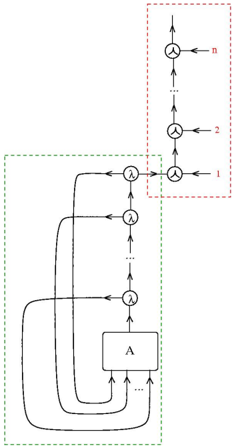
### Visual Description
## Flowchart Diagram: Control and Data Flow Processes
### Overview
The diagram illustrates two interconnected processes: a **Control Flow** sequence (top-right red box) and a **Data Flow** network (bottom-left green box). The Control Flow is a linear sequence, while the Data Flow involves iterative transformations and a central processing unit labeled "A".
---
### Components/Axes
1. **Control Flow (Red Box)**:
- **Nodes**: Labeled `n`, `2`, `1` in descending order.
- **Arrows**: Vertical downward arrows connecting nodes, indicating sequential execution.
- **Title**: "Control Flow" (top of the red box).
2. **Data Flow (Green Box)**:
- **Lambda Nodes**: Multiple instances of `λ` (lambda symbols) arranged in a loop-like structure.
- **Central Block**: Labeled "A", with multiple incoming and outgoing arrows.
- **Arrows**: Bidirectional and unidirectional connections between lambda nodes and "A".
- **Title**: "Data Flow" (top of the green box).
3. **Legend/Annotations**:
- No explicit legend, but arrow directions imply flow logic.
- Node labels (`n`, `2`, `1`, `λ`, `A`) are directly embedded in the diagram.
---
### Detailed Analysis
- **Control Flow**:
- Starts at `n` (top node) and progresses sequentially to `1` (bottom node).
- No branching or feedback loops; strictly linear.
- **Data Flow**:
- **Lambda Nodes**: Represent transformation steps. Multiple `λ` nodes feed into each other and into "A".
- **Central Block "A"**:
- Receives input from all lambda nodes.
- Outputs to multiple downstream processes (arrows exiting "A" point to unspecified targets).
- **Feedback Loop**: One lambda node (bottom-left) loops back to an earlier `λ` node, suggesting iterative processing.
---
### Key Observations
1. **Control Flow Simplicity**: The red box represents a straightforward, deterministic sequence (e.g., a loop counter from `n` to `1`).
2. **Data Flow Complexity**: The green box shows a distributed, parallelizable process with feedback, typical of algorithms requiring iterative refinement.
3. **Centralized Processing**: "A" acts as a bottleneck or aggregation point, receiving all transformed data from the lambda nodes.
---
### Interpretation
- **Control vs. Data Flow**: The diagram contrasts a simple control mechanism (red box) with a complex data-processing pipeline (green box). The control flow likely governs the number of iterations (`n`), while the data flow handles the actual computation.
- **Role of "A"**: The central block "A" could represent a critical operation (e.g., aggregation, decision-making, or output generation) that depends on all prior transformations.
- **Feedback Mechanism**: The loop in the data flow suggests adaptive or recursive behavior, such as refining results until convergence.
This diagram likely models a computational workflow where control logic (e.g., loop iterations) orchestrates a multi-stage data transformation process culminating in a centralized operation.
</details>
Packing arrows. We may pack several arrows into one. I describe first the case of two arrows. We start from the following sequence of three graphic beta moves.
<details>
<summary>Image 50 Details</summary>
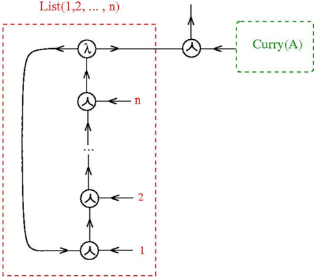
### Visual Description
## Flowchart: List Processing to Curry(A) Function
### Overview
The diagram illustrates a computational process where a list of elements (List(1, 2, ..., n)) is transformed through a series of operations (denoted by λ symbols) into numerical outputs (1, 2, ..., n), which are then aggregated into a final output labeled "Curry(A)". The flow is directional, with arrows indicating sequential dependencies.
### Components/Axes
- **Left Panel (List(1, 2, ..., n))**: A vertical list of elements labeled 1 to n, enclosed in a red dashed box.
- **Central Nodes (λ symbols)**: Five identical circular nodes labeled λ, arranged vertically. Each λ node is connected to:
- A bidirectional arrow from the list (top-to-bottom flow).
- A unidirectional arrow to a numerical output (1, 2, ..., n).
- **Right Panel (Curry(A))**: A green dashed box labeled "Curry(A)", connected to the top λ node via a unidirectional arrow.
### Detailed Analysis
1. **List(1, 2, ..., n)**:
- Positioned on the left, spanning vertically from top to bottom.
- Elements are explicitly labeled 1, 2, ..., n, with ellipsis (...) indicating continuation.
- Spatial grounding: Top of the list aligns with the top λ node; bottom aligns with the bottom λ node.
2. **λ Nodes**:
- Five identical nodes labeled λ, arranged vertically between the list and numerical outputs.
- Each λ node has:
- A bidirectional arrow from the list (input).
- A unidirectional arrow to a numerical output (output).
- Spatial grounding: λ nodes are equidistant vertically, with the top λ connected to "Curry(A)".
3. **Numerical Outputs (1, 2, ..., n)**:
- Positioned to the right of the λ nodes, aligned horizontally.
- Labels increase from 1 (bottom) to n (top), matching the list's order.
- Spatial grounding: Bottom λ node connects to "1"; top λ node connects to "n".
4. **Curry(A)**:
- Located in the top-right corner, outside the red dashed box.
- Connected only to the top λ node via a unidirectional arrow.
### Key Observations
- **Flow Direction**: Data flows from the list → λ nodes → numerical outputs → Curry(A).
- **Symmetry**: The λ nodes and numerical outputs mirror the list's structure (1 to n).
- **Curry(A) Dependency**: Only the top λ node contributes to Curry(A), suggesting a hierarchical aggregation.
### Interpretation
This diagram represents a **functional transformation pipeline**:
1. **List Processing**: Each element in List(1, 2, ..., n) is processed by a λ function (likely a lambda abstraction in programming), producing outputs 1 to n. The bidirectional arrows imply the λ operations may depend on both the input list and the output values.
2. **Currying Mechanism**: The final step, "Curry(A)", suggests the application of currying—a technique in functional programming where a function that takes multiple arguments is transformed into a sequence of functions, each taking a single argument. Here, the top λ node's output (n) may serve as the final argument to Curry(A), while lower outputs (1, 2, ..., n-1) are intermediate results.
3. **Mathematical/Computational Context**: The use of λ and currying aligns with lambda calculus and functional programming paradigms. The numerical outputs could represent indices, transformed values, or intermediate states in a recursive or iterative process.
### Notable Patterns
- **Hierarchical Aggregation**: The top λ node's exclusive connection to Curry(A) implies a prioritization or summarization of the highest-indexed element (n).
- **Bidirectional Arrows**: The λ nodes' two-way connection to the list suggests feedback loops or mutual dependencies in the transformation logic.
This diagram abstracts a computational workflow where list elements are individually transformed, aggregated, and passed to a higher-order function (Curry(A)), exemplifying principles of functional programming and mathematical abstraction.
</details>
With words, this figure means: we pack the 1, 2, entries into a list, we pass it trough one
<details>
<summary>Image 51 Details</summary>
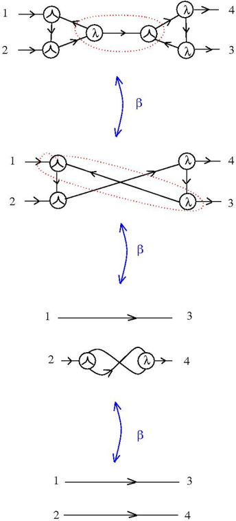
### Visual Description
## Diagram: Sequential Transformation of a Networked System
### Overview
The image depicts a three-stage transformation of a networked system represented by nodes (1–4) and directional arrows. Each stage is connected by a bidirectional arrow labeled **β**, indicating a transformation process. The diagrams evolve from a complex, interconnected structure to a simplified linear configuration, with intermediate steps involving crossed paths and dotted-line annotations.
---
### Components/Axes
1. **Nodes**: Labeled 1, 2, 3, 4 (consistent across all diagrams).
2. **Arrows**:
- **λ**: Represents directional flow or operations (e.g., "lambda" functions) between nodes.
- **β**: Indicates transformation steps between diagrams (bidirectional arrows).
3. **Dotted Lines**: Highlight alternative or optional connections in the first two diagrams.
4. **Crossed Arrows**: Appear in the second diagram, suggesting conflicting or intersecting processes.
---
### Detailed Analysis
#### Stage 1 (Top Diagram)
- **Structure**:
- Nodes 1 and 4 have outward arrows labeled **λ**.
- Nodes 2 and 3 are interconnected via bidirectional **λ** arrows.
- A dotted loop connects nodes 2 and 3, with an additional dotted arrow from node 1 to 3.
- **Key Features**:
- High connectivity; multiple feedback loops (e.g., node 2 ↔ 3).
- Dotted lines suggest non-critical or alternative pathways.
#### Stage 2 (Middle Diagram)
- **Structure**:
- Crossed arrows between nodes 1→4 and 2→3, creating an "X" pattern.
- Dotted lines now form a loop around nodes 1 and 4.
- **Key Features**:
- Increased complexity via conflicting paths (crossed arrows).
- Dotted loop emphasizes a cyclical dependency between nodes 1 and 4.
#### Stage 3 (Bottom Diagram)
- **Structure**:
- Linear flow: Node 1 → 3 and Node 2 → 4 via single **λ** arrows.
- No dotted lines or crossings.
- **Key Features**:
- Simplified, decoupled system with no feedback loops.
---
### Key Observations
1. **Progressive Simplification**: Each **β** transformation reduces complexity:
- Stage 1 → Stage 2: Adds crossed paths but retains dotted loops.
- Stage 2 → Stage 3: Eliminates all non-linear connections.
2. **Preservation of λ**: The **λ** symbols remain consistent, implying core operations are maintained despite structural changes.
3. **Dotted Lines as Anomalies**: Present only in early stages, possibly representing deprecated or optional components.
---
### Interpretation
The diagrams likely model a **system optimization process**:
- **Stage 1**: Represents an initial complex system with redundant pathways (dotted lines) and feedback loops.
- **Stage 2**: Introduces conflicts (crossed arrows) or competing processes, requiring resolution.
- **Stage 3**: Achieves a streamlined, efficient configuration by removing redundancies and conflicts.
The **β** transformations suggest iterative refinement, where each step eliminates inefficiencies while preserving essential operations (**λ**). The absence of numerical data implies a conceptual or algorithmic framework rather than empirical measurement. This could apply to fields like network theory, computational optimization, or process engineering, where simplification of interconnected systems is critical.
</details>
arrow then we unpack the list into the outputs 3, 4. This packing-unpacking trick may be used of course for more than a pair of arrows, in obvious ways, therefore it is not a restriction of generality to write only about two arrows.
We may apply the trick to a pair of graphs A and B , which are connected by a pair of arrows, like in the following figure.
<details>
<summary>Image 52 Details</summary>
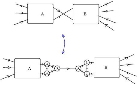
### Visual Description
## Diagram: System Interaction Flow
### Overview
The image contains two diagrams illustrating the interaction between two components labeled **A** and **B**. The top diagram shows a direct bidirectional connection between A and B via crossing arrows. The bottom diagram introduces intermediate lambda (λ) symbols between A and B, with arrows indicating a sequential flow. A blue arrow connects the two diagrams, suggesting a transformation or process from the top to the bottom representation.
### Components/Axes
- **Top Diagram**:
- **Boxes**: Labeled **A** (left) and **B** (right).
- **Arrows**: Bidirectional (X-shaped) between A and B, indicating mutual interaction.
- **Bottom Diagram**:
- **Boxes**: Same labels **A** (left) and **B** (right).
- **Lambda Symbols (λ)**: Three instances (λ₁, λ₂, λ₃) placed between A and B.
- **Arrows**: Sequential flow from A → λ₁ → λ₂ → λ₃ → B.
- **Blue Arrow**: Connects the top and bottom diagrams, pointing downward.
### Detailed Analysis
- **Top Diagram**:
- Direct, unmediated interaction between A and B.
- Arrows suggest bidirectional data exchange or mutual dependency.
- **Bottom Diagram**:
- Lambda symbols (λ) act as intermediaries or processing steps.
- Sequential arrows imply a stepwise transformation or pipeline from A to B.
- The blue arrow indicates the top diagram is a simplified abstraction, while the bottom diagram represents a detailed implementation.
### Key Observations
1. The top diagram emphasizes direct coupling between A and B.
2. The bottom diagram introduces modularity via lambda functions, suggesting a layered or decomposed system.
3. The blue arrow implies the bottom diagram is a refined or expanded version of the top diagram.
### Interpretation
The diagrams likely represent a system design evolution:
- **Top Diagram**: A high-level view of two components interacting directly, possibly in a peer-to-peer or tightly coupled architecture.
- **Bottom Diagram**: A low-level view where interactions are mediated by lambda functions (e.g., event handlers, middleware, or transformation layers). This could reflect a shift toward modularity, scalability, or separation of concerns.
- The blue arrow symbolizes the transition from a conceptual model (top) to a technical implementation (bottom), highlighting the role of intermediate processes (λ) in bridging the two components.
No numerical data or trends are present. The focus is on structural relationships and process flow.
</details>
With the added packing and unpacking triples of gates, the graphs A , B are interacting only by the intermediary of one arrow.
In particular, we may use this trick for the elementary gates of abstraction and application, transforming them into graphs with one input and one output, like this:
<details>
<summary>Image 53 Details</summary>
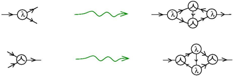
### Visual Description
## Diagram: Lambda Node Transitions and Network Structures
### Overview
The image depicts two schematic diagrams illustrating transitions between lambda (λ) nodes and complex network structures. Both diagrams feature directional arrows, lambda symbols, and green squiggly lines representing transitions. The diagrams are arranged vertically, with the top diagram showing a two-path lambda node and the bottom diagram showing a three-path lambda node.
### Components/Axes
- **Lambda Nodes (λ)**:
- Represented as circles with the Greek letter λ inside.
- Positioned at the start and end of each transition pathway.
- **Directional Arrows**:
- Black arrows indicate flow direction between nodes.
- In the top diagram, the initial λ node splits into two outgoing arrows.
- In the bottom diagram, the initial λ node splits into three outgoing arrows.
- **Green Squiggly Lines**:
- Connect the initial λ nodes to complex network structures.
- Positioned centrally between the diagrams.
- **Network Structures**:
- Top diagram: A diamond-shaped structure with four λ nodes interconnected by bidirectional arrows.
- Bottom diagram: A similar diamond-shaped structure with four λ nodes, but with a different internal arrow configuration (one central λ node with bidirectional arrows to three peripheral nodes).
### Detailed Analysis
1. **Top Diagram**:
- **Initial Node**: A single λ node with two outgoing arrows.
- **Transition**: A green squiggly line connects this node to a diamond-shaped network.
- **Network Structure**: Four λ nodes arranged in a diamond, with bidirectional arrows between adjacent nodes (forming a cycle).
2. **Bottom Diagram**:
- **Initial Node**: A single λ node with three outgoing arrows.
- **Transition**: A green squiggly line connects this node to a diamond-shaped network.
- **Network Structure**: Four λ nodes arranged in a diamond, with a central λ node connected via bidirectional arrows to three peripheral nodes (no direct connections between peripheral nodes).
### Key Observations
- The diagrams emphasize **branching pathways** (two paths in the top diagram, three in the bottom) from a single λ node to a centralized network structure.
- The **green squiggly lines** likely represent probabilistic or stochastic transitions, given their non-linear, wavy appearance.
- The **diamond-shaped networks** suggest modular or hierarchical processing, with the top diagram showing a fully connected cycle and the bottom diagram showing a star-like topology.
### Interpretation
The diagrams likely model **decision trees**, **network routing protocols**, or **probabilistic state transitions** in a computational or theoretical system. The lambda nodes (λ) could represent:
- **Decision points** with multiple outcomes (branching paths).
- **Quantum states** or **probabilistic events** in a theoretical framework.
The green squiggly lines imply **non-deterministic transitions**, possibly weighted probabilities or environmental influences. The diamond-shaped networks may represent:
- **Feedback loops** (top diagram’s cyclic connections).
- **Centralized control nodes** (bottom diagram’s star topology with a dominant central λ node).
The difference in branching (two vs. three paths) could indicate **scalability** or **complexity trade-offs** in the system. For example, the three-path diagram might represent a more complex or adaptive process compared to the two-path version.
### Notable Patterns
- **Symmetry**: Both diagrams use diamond-shaped networks, suggesting a standardized framework for processing transitions.
- **Directionality**: All arrows point toward the network structures, indicating a unidirectional flow from the initial λ node to the network.
- **Modularity**: The separation of the initial node and network structure implies modular design principles.
### Conclusion
This diagram illustrates how lambda nodes (λ) transition into complex network structures via probabilistic pathways. The differences in branching and network topology highlight variations in system complexity, adaptability, or redundancy. The use of green squiggly lines for transitions underscores the non-deterministic nature of these processes.
</details>
If we use the elementary gates transformed into graphs with one input and one output, the graphic beta move becomes this almost algebraic, 1D rule:
<details>
<summary>Image 54 Details</summary>
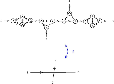
### Visual Description
## Diagram: Network Flow with Feedback Loops
### Overview
The image contains two diagrams. The top diagram is a complex network with labeled nodes (1–4), directional arrows, and symbolic annotations (λ, β). The bottom diagram is a simplified schematic with a horizontal line labeled 1–3, a vertical line labeled 2–4, and a β symbol indicating a feedback loop.
### Components/Axes
- **Top Diagram**:
- **Nodes**: Labeled 1, 2, 3, 4.
- **Arrows**:
- Black arrows with λ symbols (λ) indicating primary flow.
- Blue arrow with β symbol (β) indicating feedback.
- **Structure**:
- Node 1 connects to Node 2 via λ.
- Node 2 branches to Node 3 (λ) and Node 4 (λ).
- Node 3 connects to Node 4 via λ.
- Node 4 has a feedback loop to Node 2 via β.
- **Symbols**:
- λ: Likely represents a transformation or processing step.
- β: Represents feedback or cyclic interaction.
- **Bottom Diagram**:
- **Axes**:
- Horizontal line labeled 1 (left) and 3 (right).
- Vertical line labeled 2 (bottom) and 4 (top).
- **β Symbol**: Positioned between the horizontal and vertical lines, suggesting a feedback loop between stages 2 and 4.
### Detailed Analysis
- **Top Diagram**:
- **Flow Paths**:
- Primary flow: 1 → 2 → 3 → 4.
- Secondary flow: 2 → 4 (via λ) and 4 → 2 (via β).
- **Node 2**: Acts as a hub with multiple outgoing connections (to 3 and 4).
- **Node 4**: Receives input from Node 3 and feeds back to Node 2.
- **Bottom Diagram**:
- **β Symbol**: Positioned at the intersection of the horizontal (1–3) and vertical (2–4) lines, indicating a feedback mechanism between stages 2 and 4.
### Key Observations
1. **Feedback Loops**: The β symbol in both diagrams highlights cyclic interactions, critical for system stability or iterative processes.
2. **Node 2**: Central to both diagrams, serving as a convergence point for multiple pathways.
3. **Simplification**: The bottom diagram abstracts the top network into a minimal representation, emphasizing the feedback loop.
### Interpretation
- **System Dynamics**: The diagrams likely model a process with sequential stages (1–4) and feedback mechanisms (β). Node 2’s central role suggests it is a critical control or decision point.
- **λ vs. β**: λ may denote linear progression, while β indicates non-linear, recursive interactions.
- **Purpose**: These diagrams could represent workflows, data processing pipelines, or control systems where feedback is essential for adaptation or error correction.
**Note**: The image does not contain numerical data or explicit legends. Symbols (λ, β) and labels (1–4) are inferred from their placement and context.
</details>
With such procedures, we may transform any graph in GRAPH into a 1D string of graphs, consisting of transformed elementary graphs and packers and un-packers of arrows, which could be used, in principle, for transforming graphic lambda calculus into a text programming language.
## 5 Emergent algebras
Emergent algebras [3] [4] are a distillation of differential calculus in metric spaces with dilations [2]. This class of metric spaces contain the 'classical' riemannian manifolds, as well as fractal like spaces as Carnot groups or, more general, sub-riemannian or CarnotCarath´ eodory spaces, Bella¨ ıche [1], Gromov [11], endowed with an intrinsic differential calculus based on some variant of the Pansu derivative [18].
In [2] section 4 Binary decorated trees and dilatations, I propose a formalism for making easy various calculations with dilation structures. This formalism works with moves acting on binary decorated trees, with the leaves decorated with elements of a metric space.
Here is an example of the formalism. The moves are (with same names as those used in graphic lambda calculus, see the explanation further):
<details>
<summary>Image 55 Details</summary>
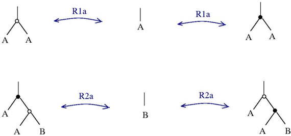
### Visual Description
## Bidirectional Transformation Diagram: Reversible Reactions R1a and R2a
### Overview
The diagram illustrates two reversible processes labeled **R1a** and **R2a**, each connecting two nodes labeled **A** and **B**. The nodes are depicted with varying circle states (open, filled, or absent), suggesting distinct states or properties. Arrows are bidirectional, indicating reversible transformations between the nodes.
### Components/Axes
- **Nodes**:
- **Top Section**:
- Left node: Labeled **A** with an open circle.
- Right node: Labeled **A** without a circle.
- **Bottom Section**:
- Left node: Labeled **A** with a filled circle.
- Right node: Labeled **B** with an open circle.
- **Arrows**:
- **R1a**: Connects the top-left node (**A** with open circle) to the top-right node (**A** without circle).
- **R2a**: Connects the bottom-left node (**A** with filled circle) to the bottom-right node (**B** with open circle).
- **Spatial Grounding**:
- Arrows are centrally positioned between nodes, emphasizing bidirectional flow.
- Circles are placed at the base of nodes, with no overlap or additional annotations.
### Detailed Analysis
- **R1a**:
- Connects two **A** nodes, one with an open circle and one without.
- Bidirectional arrow suggests a reversible transformation between these states.
- **R2a**:
- Connects **A** (filled circle) to **B** (open circle).
- Bidirectional arrow implies a reversible reaction between **A** and **B** in this configuration.
- **Circle States**:
- Open circles may represent "active" or "unmodified" states.
- Filled circles could denote "inactive" or "modified" states.
- Absence of a circle might indicate a neutral or default state.
### Key Observations
1. **Bidirectional Arrows**: Both R1a and R2a are reversible, suggesting equilibrium or dynamic balance between connected states.
2. **Node Differentiation**: The presence/absence of circles on nodes implies distinct properties or phases (e.g., active/inactive, modified/unmodified).
3. **Label Consistency**: All nodes are labeled **A** or **B**, with no additional identifiers, simplifying the system’s scope.
### Interpretation
This diagram likely represents a chemical or biological system where:
- **R1a** describes a reversible transformation between two forms of **A** (e.g., active vs. inactive states).
- **R2a** depicts a reversible reaction between **A** (modified) and **B** (unmodified), possibly involving energy exchange or catalytic processes.
- The circles may symbolize molecular conformations, binding states, or regulatory mechanisms.
- The bidirectional nature of both reactions suggests the system operates under conditions where forward and reverse processes occur simultaneously, maintaining equilibrium.
No numerical data or quantitative trends are present, so the focus remains on structural relationships and symbolic representations.
</details>
Define the following graph (and think about it as being the graphical representation of an operation u + v with respect to the basepoint x ):
<details>
<summary>Image 56 Details</summary>
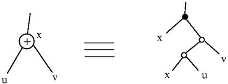
### Visual Description
## Diagram: Structural Equivalence Representation
### Overview
The image depicts two equivalent diagrammatic representations connected by a triple horizontal line (≡), indicating structural isomorphism. The left diagram shows a central node labeled "+" with three branches labeled "u," "v," and "x." The right diagram illustrates a tree-like structure with nodes labeled "x," "u," "v," and a blackened node, suggesting hierarchical relationships.
### Components/Axes
- **Left Diagram**:
- Central node: "+" (likely a root or aggregation point).
- Branches: "u," "v," "x" (direct connections to the central node).
- **Right Diagram**:
- Root node: Blackened node (no explicit label).
- Branches:
- Direct child: "x" (connected to root).
- Sub-branches from "x": "u" and "v" (nested hierarchy).
- **Equivalence Symbol**: Triple horizontal line (≡) between diagrams, denoting equivalence in structure or function.
### Detailed Analysis
- **Left Diagram**:
- The "+" node acts as a hub with equal-weight connections to "u," "v," and "x."
- No explicit hierarchy; all branches are direct and symmetric.
- **Right Diagram**:
- Hierarchical structure: Root → "x" → ("u," "v").
- The blackened node implies a distinct role (e.g., root, primary node, or special identifier).
- **Equivalence Implications**:
- The diagrams represent the same logical structure but differ in visualization (star vs. tree).
- The blackened node in the right diagram may correspond to the "+" node in the left, acting as the root.
### Key Observations
1. **Symmetry vs. Hierarchy**: The left diagram emphasizes symmetry, while the right enforces a parent-child relationship.
2. **Node Roles**: The "+" node (left) and blackened node (right) likely represent the same entity in different contexts.
3. **Label Consistency**: "u" and "v" appear in both diagrams, suggesting they are terminal or leaf nodes.
### Interpretation
This equivalence likely illustrates a concept in graph theory, data structures, or system design where different visualizations represent identical underlying relationships. The blackened node in the right diagram may denote a root or primary node, while the "+" in the left diagram abstracts this role. The equivalence symbol (≡) underscores that the structural relationships (e.g., connections between "u," "v," and "x") remain invariant despite differing representations. This could apply to scenarios like network topologies, decision trees, or organizational charts where hierarchical and flat views coexist.
</details>
Then, in the binary trees formalism I can prove, by using the moves R1a, R2a, the following 'approximate' associativity relation (it is approximate because there appear a basepoint which is different from x , but which, in the geometric context of spaces with dilations, is close to x ):
×
<details>
<summary>Image 57 Details</summary>
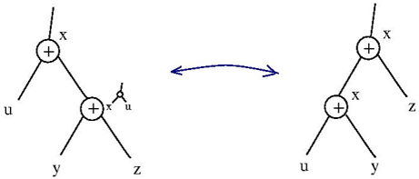
### Visual Description
## Diagram: Node Transformation Relationship
### Overview
The image depicts two interconnected diagrams via a bidirectional arrow, illustrating a transformation or equivalence relationship between two node-based structures. Both diagrams use labeled nodes (+, x, u, y, z) with directional edges.
### Components/Axes
- **Nodes**:
- Left Diagram:
- Top node: `+` (root)
- Left child of `+`: `u`
- Right child of `+`: `x` (with a smaller `+x` node branching to `u`)
- Children of `x`: `y` and `z`
- Right Diagram:
- Top node: `+` (root)
- Left child of `+`: `x` (connected to `u`)
- Right child of `+`: `x` (connected to `z`)
- Children of `x` (right branch): `y`
- **Edges**:
- Solid lines represent parent-child relationships.
- Bidirectional arrow (`↔`) connects the two diagrams, indicating a reversible transformation.
### Detailed Analysis
- **Left Diagram**:
- The root `+` splits into `u` (left) and `x` (right).
- The `x` node has a sub-node `+x` (smaller circle) branching to `u`, suggesting a recursive or nested structure.
- `x` also connects to `y` and `z` as terminal nodes.
- **Right Diagram**:
- The root `+` splits into two `x` nodes:
- Left `x` connects to `u`.
- Right `x` connects to `z` and `y`.
- No nested `+x` sub-node is present.
### Key Observations
1. **Structural Symmetry**: Both diagrams share the same set of labels (`u, x, y, z`) but differ in node connections.
2. **Bidirectional Relationship**: The arrow implies the transformation between the diagrams is reversible (e.g., a mathematical isomorphism or algorithmic operation).
3. **Nested Node**: The left diagram’s `+x` sub-node introduces a hierarchical layer absent in the right diagram.
### Interpretation
The diagrams likely represent a computational or mathematical transformation, such as:
- **Tree Rotation**: Rearranging nodes while preserving relationships (e.g., balancing a binary tree).
- **Graph Isomorphism**: Demonstrating equivalence between two structures under specific operations.
- **Algorithmic Step**: Illustrating a before/after state in a process (e.g., data restructuring).
The absence of numerical values suggests the focus is on topological or logical relationships rather than quantitative data. The bidirectional arrow emphasizes reversibility, critical in contexts like reversible computing or reversible logic circuits.
</details>
It was puzzling that in fact the formalism worked without needing to know which metric space is used. Moreover, reasoning with moves acting on binary trees gave proofs of generalizations of results from sub-riemannian geometry, while classical proofs involve elaborate calculations with pseudo-differential operators. At a close inspection it looked like some-
where in the background there is an abstract nonsense machine which is just applied to the particular case of sub-riemannian spaces.
In this paper I shall take the following pure algebraic definition of an emergent algebra (compare with definition 5.1 [3]), which is a stronger version of the definition 4.2 [4] of a Γ idempotent right quasigroup, in the sense that here I define a Γ idempotent quasigroup.
Definition 5.1 Let Γ be a commutative group with neutral element denoted by 1 and operation denoted multiplicatively. A Γ idempotent quasigroup is a set X endowed with a family of operations ◦ ε : X × X → X , indexed by ε ∈ Γ , such that:
- -For any ε ∈ Γ \ { 1 } the pair ( X, ◦ ε ) is an idempotent quasigroup, i.e. for any a, b ∈ X the equations x ◦ ε a = b and a ◦ ε x = b have unique solutions and moreover x ◦ ε x = x for any x ∈ X ,
- -The operation ◦ 1 is trivial: for any x, y ∈ X we have x ◦ 1 y = y ,
- -For any x, y ∈ X and any ε, µ ∈ Γ we have: x ◦ ε ( x ◦ µ y ) = x ◦ εµ y .
Here are some examples of Γ idempotent quasigroups.
Example 1. Real (or complex) vector spaces: let X be a real (complex) vector space, Γ = (0 , + ∞ ) (or Γ = C ∗ ), with multiplication as operation. We define, for any ε ∈ Γ the following quasigroup operation: x ◦ ε y = (1 -ε ) x + εy . These operations give to X the structure of a Γ idempotent quasigroup. Notice that x ◦ ε y is the dilation based at x , of coefficient ε , applied to y .
Example 2. Contractible groups: let G be a group endowed with a group morphism φ : G → G . Let Γ = Z with the operation of addition of integers (thus we may adapt definition 5.1 to this example by using ' ε + µ ' instead of ' εµ ' and '0' instead of '1' as the name of the neutral element of Γ). For any ε ∈ Z let x ◦ ε y = xφ ε ( x -1 y ). This a Z idempotent quasigroup. The most interesting case is the one when φ is an uniformly contractive automorphism of a topological group G . The structure of these groups is an active exploration area, see for example [12] and the bibliography therein. A fundamental result here is Siebert [20], which gives a characterization of topological connected contractive locally compact groups as being nilpotent Lie groups endowed with a one parameter family of dilations, i.e. almost Carnot groups.
Example 3. A group with an invertible self-mapping φ : G → G such that φ ( e ) = e , where e is the identity of the group G . It looks like Example 2 but it shows that there is no need for φ to be a group morphism.
Local versions. We may accept that there is a way (definitely needing care to well formulate, but intuitively clear) to define a local version of the notion of a Γ idempotent quasigroup. With such a definition, for example, a convex subset of a real vector space gives a local (0 , + ∞ ) idempotent quasigroup (as in Example 1) and a neighbourhood of the identity of a topological group G , with an identity preserving, locally defined invertible self map (as in Example 3) gives a Z local idempotent quasigroup.
Example 4. A particular case of Example 3 is a Lie group G with the operations defined for any ε ∈ (0 , + ∞ ) by x ◦ ε y = x exp( ε log( x -1 y )).
Example 5. A less symmetric example is the one of X being a riemannian manifold, with associated operations defined for any ε ∈ (0 , + ∞ ) by x ◦ ε y = exp x ( ε log x ( y )), where exp is the metric exponential.
Example 6. More generally, any metric space with dilations is a local idempotent (right) quasigroup.
Example 7. One parameter deformations of quandles. A quandle is a self-distributive quasigroup. Take now a one-parameter family of quandles (indexed by ε ∈ Γ) which satisfies moreover points 2. and 3. from definition 5.1. What is interesting about this example is that quandles appear as decorations of knot diagrams [10] [13], which are preserved by the Reidemeister moves (more on this in the section 6). At closer examination, examples 1, 2 are particular cases of one parameter quandle deformations!
I define now the operations of approximate sum and approximate difference associated to a Γ idempotent quasigroup.
Definition 5.2 For any ε ∈ Γ we give the following names to several combinations of operations of emergent algebras:
- -the approximate sum operation is Σ x ε ( u, v ) = x · ε (( x ◦ ε u ) ◦ ε v ) ,
- -the approximate difference operation is ∆ x ε ( u, v ) = ( x ◦ ε u ) · ε ( x ◦ ε v ) ,
- -the approximate inverse operation is inv x ε u = ( x ◦ ε u ) · ε x .
Let's see what the approximate sum operation is, for example 1.
$$2 ^ { 3 } ( 1 0 , 0 ) = 4 0 ( - 0 ) - 8 + 0$$
It is clear that, as ε converges to 0, this becomes the operation of addition in the vector space with x as neutral element, so it might be said that is the operation of addition of vectors in the tangent space at x , where x is seen as an element of the affine space constructed over the vector space from example 1.
This is a general phenomenon, which becomes really interesting in non-commutative situations, i.e. when applied to examples from the end of the provided list.
These approximate operations have many algebraic properties which can be found by the abstract nonsense of manipulating binary trees.
Another construction which can be done in emergent algebras is the one of taking finite differences (at a high level of generality, not bonded to vector spaces).
Definition 5.3 Let A : X → X be a function (from X to itself, for simplicity). The finite difference function associated to A , with respect to the emergent algebra over X , at a point x ∈ X is the following.
$$u ) = A ( x ) \cdot e ^ { ( A ( x o _ { e } u ) ) }$$
For example 1, the finite difference has the expression:
$$T _ { e } A ( u - x ) = A ( x ) +$$
which is a finite difference indeed. In more generality, for example 2 this definition leads to the Pansu derivative [18].
Finite differences as defined here behave like discrete versions of derivatives. Again, the proofs consist in manipulating well chosen binary trees.
All this can be formalized in graphic lambda calculus, thus transforming the proofs into computations inside graphic lambda calculus.
I shall not insist more on this, with the exception of describing the emergent algebra sector of graphic lambda calculus.
Definition 5.4 For any ε ∈ Γ , the following graphs in GRAPH are introduced:
- -the approximate sum graph Σ ε
<details>
<summary>Image 58 Details</summary>
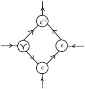
### Visual Description
## Diagram: Cyclic System with Inverse Element
### Overview
The image depicts a directed cyclic graph with four nodes arranged in a diamond (quadrilateral) structure. Arrows indicate directional flow between nodes, forming a closed loop. Labels on nodes include the Greek letter epsilon (ε) and its inverse (ε⁻¹).
### Components/Axes
- **Nodes**:
- Top node: Labeled **ε⁻¹** (inverse epsilon).
- Right node: Labeled **ε**.
- Bottom node: Labeled **ε**.
- Left node: Labeled **ε** (with a bifurcation symbol, resembling a "Y" or split).
- **Edges**:
- Arrows connect nodes in a clockwise cycle:
1. **ε⁻¹ → ε** (top to right).
2. **ε → ε** (right to bottom).
3. **ε → ε** (bottom to left).
4. **ε → ε⁻¹** (left to top).
- **Legend**: None explicitly visible.
### Detailed Analysis
- **Node Labels**:
- Three nodes are labeled **ε**, while one node is labeled **ε⁻¹**. The inverse notation (ε⁻¹) suggests a mathematical or operational relationship (e.g., multiplicative inverse, reverse process).
- The left node’s bifurcation symbol may imply a branching or dual-path mechanism in the system.
- **Flow Direction**:
- The cycle is unidirectional, with all edges pointing clockwise. This implies a deterministic or sequential process.
- The inverse element (ε⁻¹) acts as both a starting and ending point, creating a feedback loop.
### Key Observations
1. **Cyclic Dependency**: The system forms a closed loop, indicating interdependence between nodes.
2. **Inverse Element**: The presence of ε⁻¹ suggests a reversal or balancing mechanism within the cycle.
3. **Bifurcation**: The left node’s split symbol could represent divergence in pathways or states.
### Interpretation
This diagram likely represents a theoretical or mathematical system where:
- **ε** denotes a standard state or operation.
- **ε⁻¹** represents an inverse or compensatory action, critical for maintaining equilibrium in the cycle.
- The bifurcation at the left node may indicate a decision point or parallel processing step.
The closed-loop structure implies that the system is self-sustaining, with outputs feeding back into inputs. The inverse element (ε⁻¹) could symbolize a corrective or stabilizing force, ensuring the cycle persists without external intervention. The bifurcation introduces complexity, suggesting potential for multiple outcomes or states within the system.
No numerical data or quantitative trends are present; the focus is on structural relationships and symbolic labels.
</details>
-the approximate difference graph ∆ ε
<details>
<summary>Image 59 Details</summary>
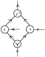
### Visual Description
## Diagram: State Transition Network with Inverse and Y-Junction
### Overview
The diagram depicts a directed graph with four nodes connected by arrows, forming a network with cyclic and acyclic paths. Key elements include three nodes labeled **ε**, one node labeled **ε⁻¹**, and a Y-shaped node labeled **Y**. Arrows indicate directional relationships between nodes.
### Components/Axes
- **Nodes**:
- Top node: **ε⁻¹** (inverse of ε).
- Right node: **ε**.
- Left node: **ε**.
- Bottom node: **Y** (Y-shaped symbol).
- **Arrows**:
- **ε⁻¹ → ε** (top to right).
- **ε → Y** (right to bottom).
- **ε → Y** (left to bottom).
- **Y → ε** (bottom to left).
- **Y → ε** (bottom to right).
- **ε → ε** (left to right, horizontal).
### Detailed Analysis
- **Node Labels**:
- Three nodes are labeled **ε** (standard symbol, possibly representing a unit or identity element).
- One node is labeled **ε⁻¹** (inverse of ε, suggesting a reverse operation or starting point).
- The Y-shaped node is unlabeled but distinct in shape, acting as a junction.
- **Flow Directions**:
- The **ε⁻¹** node initiates a path to the right **ε** node.
- Both **ε** nodes (left and right) connect to the **Y** node.
- The **Y** node splits into two outgoing arrows, feeding back into the left and right **ε** nodes.
- A horizontal arrow connects the left **ε** node to the right **ε** node.
### Key Observations
1. **Cyclic Paths**:
- The **Y** node forms a loop with both **ε** nodes (left and right), creating bidirectional dependencies.
2. **Inverse Element**:
- The **ε⁻¹** node suggests an initial or reverse state, contrasting with the standard **ε** nodes.
3. **Y-Junction Behavior**:
- The **Y** node acts as a central hub, merging inputs from both **ε** nodes and distributing outputs back to them.
### Interpretation
This diagram likely represents a **state transition system** or **process flow** with the following implications:
- **Mathematical Context**: If **ε** represents a generator in group theory, **ε⁻¹** could denote its inverse, and the **Y** node might symbolize a relation or constraint (e.g., commutativity).
- **Process Workflow**: The **Y** node could represent a decision point where paths diverge or converge, with feedback loops enabling iterative processes.
- **Anomalies**: The horizontal arrow between **ε** nodes (left to right) introduces a direct connection outside the **Y**-mediated cycles, potentially signifying a shortcut or alternative pathway.
The structure emphasizes interdependence between nodes, with the **Y** node central to maintaining balance between cyclic and acyclic transitions. The presence of **ε⁻¹** highlights asymmetry in the system’s initialization or termination states.
</details>
-the approximate inverse graph inv ε
<details>
<summary>Image 60 Details</summary>
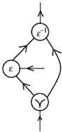
### Visual Description
## Diagram: Directed Graph with Three Nodes
### Overview
The image depicts a directed graph with three nodes connected by arrows. The nodes are labeled with symbols: **ε⁻¹** (top), **ε** (middle-left), and **Y** (bottom). Arrows indicate directional relationships between the nodes, with a bifurcation at node **Y**.
### Components/Axes
- **Nodes**:
- **ε⁻¹**: Positioned at the top, connected to **ε** via a leftward arrow.
- **ε**: Located in the middle-left, connected to **Y** via a rightward arrow.
- **Y**: Positioned at the bottom, with a split arrow (bifurcation) pointing downward.
- **Arrows**:
- **ε⁻¹ → ε**: Leftward arrow.
- **ε → Y**: Rightward arrow.
- **Y**: Split arrow (no explicit label for the bifurcation paths).
### Detailed Analysis
- **Node Labels**:
- **ε⁻¹**: Likely represents an inverse element (mathematical or symbolic context).
- **ε**: A central node, possibly denoting a base or reference state.
- **Y**: A terminal node with a bifurcation, suggesting divergence into two paths.
- **Flow Direction**:
- The graph starts at **ε⁻¹**, flows to **ε**, then to **Y**, where it splits.
- No numerical values or scales are present; the diagram is purely structural.
### Key Observations
1. **Directional Flow**: The graph enforces a strict sequence: **ε⁻¹ → ε → Y**, with no feedback loops.
2. **Bifurcation at Y**: The split arrow at **Y** implies two possible outcomes or states post-**Y**, though the paths are unlabeled.
3. **Symbolic Labels**: The use of **ε** and **ε⁻¹** suggests a mathematical or abstract system (e.g., group theory, logic).
### Interpretation
This diagram likely models a process or system with a defined sequence leading to a decision point (**Y**). The inverse relationship between **ε⁻¹** and **ε** could imply a reversible or complementary interaction (e.g., input-output dynamics, cause-effect chains). The bifurcation at **Y** introduces ambiguity, requiring further context to interpret the downstream paths. The absence of numerical data or labels on the split paths limits quantitative analysis, emphasizing the diagram’s role in illustrating structural relationships rather than quantitative trends.
</details>
Let A be a set of symbols a, b, c, ... . (These symbols will play the role of scale parameters going to 0.) With A and with the abelian group Γ we construct a larger abelian group, call it ¯ Γ, which is generated by A and by Γ.
Now we introduce the emergent algebra sector (over the set A ).
Definition 5.5 EMER ( A ) is the subset of GRAPH (over the group ¯ Γ ) which is generated by the following list of gates:
- -arrows and loops,
- -Υ gate and the gates ¯ ε for any ε ∈ Γ ,
- -the approximate sum gate Σ a and the approximate difference gate ∆ a , for any a ∈ A ,
with the operations of linking output to input arrows and with the following list of moves:
- FAN-OUT moves
- -emergent algebra moves for the group ¯ Γ ,
- -¡pruning moves.
The set EMER ( A ) with the given list of moves is called the emergent algebra sector over the set A .
The approximate inverse is not included into the list of generating gates. That is because we can prove easily that for any a ∈ A we have inv a ∈ EMER ( A ). (If ε ∈ Γ then we trivially have inv ε ∈ EMER ( A ) because it is constructed from emergent algebra gates decorated by elements in Γ, which are on the list of generating gates.) Here is the proof: we start with the approximate difference ∆ a and with an Υ gate and we arrive to the approximate inverse inv a by a sequence of moves, as follows.
<details>
<summary>Image 61 Details</summary>
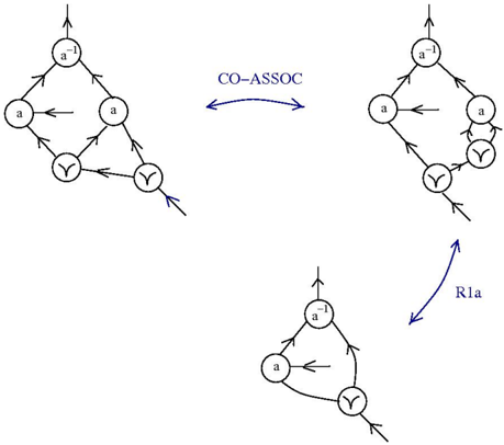
### Visual Description
## Diagram: State Transition and Interaction Models
### Overview
The image depicts three interconnected diagrams labeled **CO-ASSOC**, **R1a**, and a simplified third diagram. Each diagram consists of nodes labeled **a**, **a⁻¹**, and **Y**, connected by directional arrows. The diagrams illustrate relationships or transitions between these nodes, with varying arrow configurations.
### Components/Axes
- **Nodes**:
- **a**: Represented as a circle with a label "a".
- **a⁻¹**: Represented as a circle with a label "a⁻¹" (inverse of "a").
- **Y**: Represented as a circle with a label "Y".
- **Arrows**:
- **Bidirectional arrows** (e.g., between **a** and **a⁻¹** in CO-ASSOC).
- **Unidirectional arrows** (e.g., from **a** to **Y** in CO-ASSOC and R1a).
- **Labels**:
- **CO-ASSOC**: Indicates a co-association or mutual relationship.
- **R1a**: Likely a specific interaction or rule (e.g., "Rule 1a").
### Detailed Analysis
1. **CO-ASSOC Diagram**:
- **Nodes**: **a**, **a⁻¹**, and **Y**.
- **Arrows**:
- **a ↔ a⁻¹**: Bidirectional arrows suggest a mutual or reciprocal relationship.
- **a → Y**: Unidirectional arrow from **a** to **Y**, indicating a one-way influence or transition.
- **Structure**: Forms a triangular configuration with **Y** connected to **a**.
2. **R1a Diagram**:
- **Nodes**: **a**, **a⁻¹**, and **Y**.
- **Arrows**:
- **a → a⁻¹**: Unidirectional arrow from **a** to **a⁻¹**.
- **a⁻¹ → Y**: Unidirectional arrow from **a⁻¹** to **Y**.
- **Y → a**: Unidirectional arrow from **Y** back to **a**, forming a cycle.
- **Structure**: A linear chain with a feedback loop from **Y** to **a**.
3. **Simplified Diagram**:
- **Nodes**: **a**, **a⁻¹**, and **Y**.
- **Arrows**:
- **a → a⁻¹**: Unidirectional arrow from **a** to **a⁻¹**.
- **a⁻¹ → Y**: Unidirectional arrow from **a⁻¹** to **Y**.
- **Structure**: A linear flow without feedback.
### Key Observations
- **CO-ASSOC** emphasizes mutual relationships (bidirectional arrows) and a direct influence of **a** on **Y**.
- **R1a** introduces a cyclic dependency, where **Y** feeds back into **a**, creating a closed loop.
- The simplified diagram removes the feedback loop, suggesting a linear or sequential process.
### Interpretation
The diagrams likely represent different states or interaction models in a system:
- **CO-ASSOC** could model a co-association where **a** and **a⁻¹** are interdependent, with **Y** being influenced by **a**.
- **R1a** might represent a rule or process where **a** transitions to **a⁻¹**, which then affects **Y**, which in turn influences **a** again, creating a self-reinforcing cycle.
- The simplified diagram may illustrate a baseline or initial state without feedback mechanisms.
The presence of **a⁻¹** (inverse of **a**) suggests a focus on reciprocal or inverse relationships, possibly in mathematical, logical, or computational contexts. The directional arrows highlight causality or influence, while the labels **CO-ASSOC** and **R1a** imply specific rules or associations governing these interactions.
</details>
We proved the following relation for emergent algebras: ∆ x a ( u, x ) = inv x a u . This relation appears as a computation in graphic lambda calculus.
As for the finite differences, we may proceed as this.
Definition 5.6 A graph A ∈ GRAPH , with one input and one output distinguished, is computable with respect to the group ¯ Gamma if the following graph
<details>
<summary>Image 62 Details</summary>
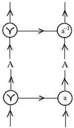
### Visual Description
## Diagram: Y-shaped Nodes with Inverse Operations
### Overview
The diagram depicts two Y-shaped nodes connected by directional arrows, with labels indicating operations and their inverses. The structure suggests a flow or transformation process involving an operation (`A`) and its inverse (`A⁻¹`).
### Components/Axes
- **Y-shaped Nodes**: Two identical nodes labeled with a "Y" symbol, each having two incoming arrows and one outgoing arrow.
- **Arrows**:
- Two arrows point **upward** into each Y-shaped node.
- One arrow points **rightward** from each Y-shaped node to a labeled node.
- **Labeled Nodes**:
- Top-right node: Labeled `A⁻¹` (inverse of `A`).
- Bottom-right node: Labeled `A`.
- **Directionality**: All arrows indicate unidirectional flow (no bidirectional or feedback loops).
### Detailed Analysis
- **Top Pathway**:
- Two inputs (upward arrows) feed into the top Y-shaped node.
- Output flows rightward to the node labeled `A⁻¹`.
- **Bottom Pathway**:
- Two inputs (upward arrows) feed into the bottom Y-shaped node.
- Output flows rightward to the node labeled `A`.
- **Symmetry**: The two Y-shaped nodes are identical in structure, suggesting parallel or mirrored processes.
### Key Observations
1. The labels `A` and `A⁻¹` imply a relationship where one operation is the inverse of the other.
2. The Y-shaped nodes act as intermediaries, combining two inputs into a single output.
3. No numerical values, scales, or legends are present; the diagram is purely symbolic.
### Interpretation
This diagram likely represents a **functional or algorithmic process** where:
- The Y-shaped nodes symbolize a **combining operation** (e.g., merging two inputs into a single output).
- The labels `A` and `A⁻¹` suggest a **transformation and its inverse**, possibly indicating reversible steps in a workflow.
- The symmetry between the two pathways implies **parallel processing** or **dual operations** (e.g., forward and reverse transformations).
The absence of numerical data or additional context limits quantitative analysis, but the structure emphasizes **directional flow** and **operational relationships**.
</details>
can be transformed by the moves from graphic lambda calculus into a graph which is made by assembling:
- -graphs from EMER ( A ) ,
- -gates λ , and .
It would be interesting to mix the emergent algebra sector with the lambda calculus sector (in a sense this is already suggested in definition 5.6). At first view, it seems that the emergent algebra gates ¯ ε are operations which are added to the lambda calculus operations, the latter being more basic than the former. I think this is not the case. In [5] theorem 3.4, in the formalism of lambda-scale calculus (graphic lambda calculus is a visual variant of this), I
show on the contrary that the emergent algebra gates could be applied to lambda terms and the result is a collection, or hierarchy of lambda calculi, organized into an emergent algebra structure. This is surprising, at least for the author, because the initial goal of introducing lambda-scale calculus was to mimic lambda calculus with emergent algebra operations.
## 6 Crossings
In this section we discuss about tangle diagrams and graphic lambda calculus.
An oriented tangle is a collection of wired in 3D space, more precisely it is an embedding of a oriented one dimensional manifold in 3D space. Two tangles are the same up to topological deformation of the 3D space. An oriented tangle diagram is, visually, a projection of a tangle, in general position, on a plane. More specifically, an oriented tangle diagram is a globally planar oriented graph with 4-valent nodes which represent crossings of wires (as seen in the projection), along with supplementary information about which wire passes over the respective crossing. A locally planar tangle diagram is an oriented graph which satisfies the previous description, with the exception that it is only locally planar. Visually, a locally planar tangle diagram looks like an ordinary one, excepting that there may be crossings of edges of the graph which are not tangle crossings (i.e. nodes of the graph).
The purpose of this section is to show that we can 'simulate' tangle diagrams with graphic lambda calculus. This can be expressed more precisely in two ways. The first way is that we can define 'crossing macros' in graphic lambda calculus, which are certain graphs which play the role of crossings in a tangle diagram (i.e. we can express the Reidemeister moves, described further, as compositions of moves from graphic lambda calculus between such graphs). The second way is to say that to any tangle diagram we can associate a graph in GRAPH such that to any Reidemeister move is associated a certain composition of moves from graphic lambda calculus.
Meredith ad Snyder [17] achieve this goal with the pi-calculus instead of graphic lambda calculus. Kauffman, in the second part of [14], associates tangle diagrams to combinators and writes about 'knotlogic'.
Oriented Reidemeister moves. Two tangles are the same, up to topological equivalence, if and only if any tangle diagram of one tangle can be transformed by a finite sequence of Reidemeister moves into a tangle diagram of the second tangle. The oriented Reidemeister moves are the following (I shall use the same names as Polyak [19], but with the letter Ω replaced by the letter R ):
- -four oriented Reidemeister moves of type 1:
- -four oriented Reidemeister moves of type 2:
<details>
<summary>Image 63 Details</summary>
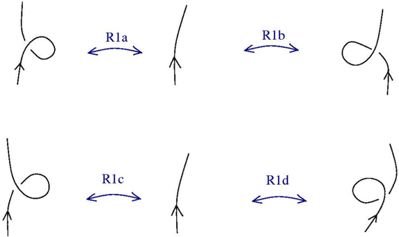
### Visual Description
## Diagram: Transformation Process of Looped Lines to Straight Lines
### Overview
The image contains four diagrams arranged in a 2x2 grid, each illustrating a transformation process from a looped line to a straight line. Arrows indicate the direction of transformation, labeled as R1a, R1b, R1c, and R1d.
### Components/Axes
- **Diagrams**:
- **Top Row**:
- **Left (R1a)**: A looped line (leftward arrow) transforms into a straight line (downward arrow).
- **Right (R1b)**: A looped line (rightward arrow) transforms into a straight line (downward arrow).
- **Bottom Row**:
- **Left (R1c)**: A looped line (leftward arrow) transforms into a straight line (downward arrow).
- **Right (R1d)**: A looped line (rightward arrow) transforms into a straight line (downward arrow).
- **Labels**:
- R1a, R1b, R1c, R1d (blue text, centered between looped and straight lines).
- **Arrows**:
- Directional arrows (black) indicate transformation flow.
### Detailed Analysis
- **R1a**: Looped line (leftward) → Straight line (downward).
- **R1b**: Looped line (rightward) → Straight line (downward).
- **R1c**: Looped line (leftward) → Straight line (downward).
- **R1d**: Looped line (rightward) → Straight line (downward).
- **Spatial Grounding**:
- Labels (R1a-R1d) are centrally positioned between the looped and straight lines.
- Arrows are placed at the ends of the lines to denote direction.
### Key Observations
1. All transformations result in a straight line with a downward arrow, regardless of the initial looped line's direction.
2. The looped lines in R1a and R1c share identical directional arrows (leftward), while R1b and R1d share rightward arrows.
3. No numerical data, scales, or legends are present.
### Interpretation
The diagrams likely represent a conceptual or procedural flow, where each R1 label denotes a distinct transformation step or category. The consistent downward arrow in the final straight lines suggests a unified outcome or endpoint across all processes. The variation in initial looped line directions (left/right) may indicate different input conditions or scenarios leading to the same result. The absence of quantitative data implies this is a schematic representation rather than a statistical analysis.
</details>
<details>
<summary>Image 64 Details</summary>
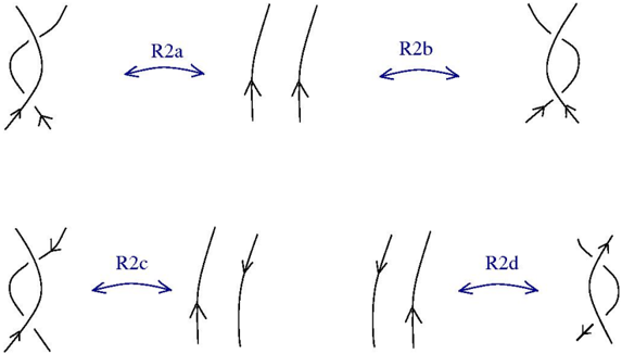
### Visual Description
## Diagram: Network Configuration Relationships
### Overview
The image presents four interconnected diagrams (R2a-R2d) illustrating network topology transformations. Each diagram uses arrows and line configurations to represent directional relationships between nodes or pathways.
### Components/Axes
- **Diagrams**:
- Top Row: R2a (left), R2b (right)
- Bottom Row: R2c (left), R2d (right)
- **Visual Elements**:
- Curved lines with arrowheads
- Parallel straight lines with directional arrows
- Central nodes (implied by arrow origins)
- **Labels**:
- R2a, R2b, R2c, R2d (blue text with bidirectional arrows between diagrams)
### Detailed Analysis
1. **R2a**:
- Single curved line with two outward-pointing arrows from a central node
- Arrows diverge at 45° angles from the line's midpoint
2. **R2b**:
- Two parallel straight lines with inward-pointing arrows
- Arrows converge toward a central point between the lines
3. **R2c**:
- Single straight line with two outward-pointing arrows
- Arrows diverge at 90° angles from the line's endpoints
4. **R2d**:
- Two parallel lines with outward-pointing arrows
- Arrows diverge at 45° angles from each line's midpoint
### Key Observations
- **Directional Symmetry**: R2a and R2c show outward divergence, while R2b demonstrates inward convergence
- **Line Configuration**: R2b and R2d use parallel lines, whereas R2a and R2c use single lines
- **Arrow Angles**: R2c has the sharpest divergence (90°), while R2a/R2d use 45° angles
- **Node Implication**: Central nodes are implied in R2a/R2b but not explicitly shown in R2c/R2d
### Interpretation
These diagrams likely represent:
1. **Network Topology Variations**:
- R2a/R2c: Star-like configurations with central hubs
- R2b: Mesh-like interconnection with bidirectional flow
- R2d: Dual-path redundancy system
2. **Process Flow Models**:
- R2b's convergence suggests decision-making nodes
- R2d's parallel paths imply load balancing
3. **Critical Relationships**:
- R2a ↔ R2c: Transition from curved to straight pathways
- R2b ↔ R2d: Shift from convergence to divergence in parallel systems
The absence of explicit nodes in R2c/R2d suggests these configurations might represent end-state transformations of the earlier models. The consistent use of bidirectional arrows between diagrams indicates these are reversible processes or equivalent states in a network evolution framework.
</details>
-eight oriented Reidemeister moves of type 3:
<details>
<summary>Image 65 Details</summary>
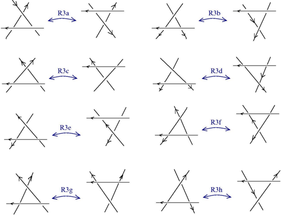
### Visual Description
## Diagram: Arrow Configuration Transformations
### Overview
The image displays a grid of eight diagrams (2x4 layout) illustrating transformations between arrow configurations. Each diagram is labeled with a unique identifier (e.g., R3a, R3b) and shows directional arrows intersecting or diverging. Arrows are depicted with directional indicators (→, ←, ↑, ↓) and spatial relationships (e.g., crossing, parallel, opposing).
### Components/Axes
- **Labels**:
- R3a, R3b, R3c, R3d, R3e, R3f, R3g, R3h (eight distinct configurations).
- **Arrow Directions**:
- Arrows are annotated with directional symbols (→, ←, ↑, ↓) to indicate flow or orientation.
- **Spatial Relationships**:
- Arrows intersect, diverge, or align in specific patterns (e.g., crossing, parallel, opposing).
### Detailed Analysis
1. **R3a**: Two arrows cross diagonally (↗ and ↖), with a horizontal line below.
2. **R3b**: Two arrows point in opposite horizontal directions (→ and ←), with a horizontal line above.
3. **R3c**: Two arrows form a V-shape (↗ and ↙), with a horizontal line below.
4. **R3d**: Two arrows cross diagonally (↘ and ↖), with a horizontal line above.
5. **R3e**: Two arrows form an X-shape (↗ and ↙), with a horizontal line below.
6. **R3f**: Two arrows cross diagonally (↘ and ↖), with a horizontal line below.
7. **R3g**: Two arrows form a V-shape (↗ and ↙), with a horizontal line above.
8. **R3h**: Two arrows cross diagonally (↘ and ↖), with a horizontal line below.
### Key Observations
- **Directional Variability**: Arrows alternate between horizontal, diagonal, and V-shaped configurations.
- **Label Consistency**: All labels follow the "R3X" format (X = a–h), suggesting a systematic categorization.
- **Spatial Patterns**: Horizontal lines appear in all diagrams, either above or below the arrow intersections.
### Interpretation
The diagrams likely represent states or steps in a process where directional relationships (e.g., alignment, opposition) between variables or components are critical. The horizontal line may symbolize a baseline or reference point. The systematic labeling (R3a–R3h) implies a structured framework for analyzing transformations, possibly in fields like physics, engineering, or systems theory. No numerical data is present, so trends or outliers cannot be quantified.
</details>
Crossings from emergent algebras. In section 5, example 7, it is mentioned that there is a connection between tangle diagrams and emergent algebras, via the notion of a quandle. Quandles are self-distributive idempotent quasigroups, which were invented as decorations of the arrows of a tangle diagram, which are invariant with respect to the Reidemeister moves.
Let us define the emergent algebra crossing macros. (We can choose to neglect the ε decorations of the crossings, or, on the contrary, we can choose to do like in definition 5.5 of the emergent algebra sector, namely to add a set A to the group Γ and use even more nuanced decorations for the crossings.)
<details>
<summary>Image 66 Details</summary>
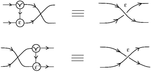
### Visual Description
## Diagram: Algebraic Structure Transformation
### Overview
The image contains two pairs of diagrams connected by equivalence symbols (≡). Each pair demonstrates a transformation from a complex network of nodes and arrows to a simplified representation. The diagrams use symbolic notation (Y, ε, ε⁻¹) and directional arrows to illustrate relationships.
### Components/Axes
- **Nodes**:
- **Y**: Represented as a circle with two downward arrows (top diagram) and a single downward arrow (bottom diagram).
- **ε**: Labeled as a circle with a single downward arrow (top diagram).
- **ε⁻¹**: Labeled as a circle with a single upward arrow (bottom diagram).
- **Arrows**:
- Directional arrows connect nodes, indicating flow or transformation.
- Crossed arrows (✘) appear in the simplified right-side diagrams.
- **Equivalence Symbols**:
- Three horizontal lines (≡) separate the left and right diagrams in each pair.
### Detailed Analysis
1. **Top Diagram Pair**:
- **Left**: Two Y nodes connected by bidirectional arrows, with ε nodes below each Y.
- **Right**: Simplified to a single ε node with crossed arrows (✘).
- **Key Text**: "ε" labeled on the right diagram.
2. **Bottom Diagram Pair**:
- **Left**: A Y node connected to an ε⁻¹ node via bidirectional arrows.
- **Right**: Simplified to a single ε⁻¹ node with crossed arrows (✘).
- **Key Text**: "ε⁻¹" labeled on the right diagram.
### Key Observations
- The left diagrams show interconnected nodes (Y and ε/ε⁻¹) with complex relationships.
- The right diagrams reduce these to single nodes (ε or ε⁻¹) with crossed arrows, suggesting cancellation or simplification.
- The equivalence symbols (≡) imply that the left and right diagrams represent the same structure under specific rules.
### Interpretation
The diagrams likely represent a mathematical or categorical equivalence, such as:
- **Group Theory**: The Y nodes could represent generators, and ε/ε⁻¹ relations that simplify the group structure.
- **Category Theory**: The transformation might illustrate an isomorphism or equivalence between complex and simplified functors.
- **Topological Algebra**: The crossed arrows (✘) may denote null homotopy or cancellation of loops.
The simplification from left to right suggests that the complex network of nodes and arrows collapses to a single generator (ε or ε⁻¹) under defined equivalence rules. This could model processes like quotienting, homotopy, or algebraic reduction.
No numerical data or trends are present; the focus is on symbolic relationships and structural equivalence.
</details>
In [6], sections 3-6 are dedicated to the use of these crossings for exploring emergent algebras and spaces with dilations. All constructions and reasonings from there can be put into the graphic lambda calculus formalism. Here I shall explain only some introductory facts.
Let us associate to any locally planar tangle diagram T a graph in [ T ] ∈ GRAPH , called the translation of T , which is obtained by replacing the crossings with the emergent crossing macros (for a fixed ε ). Also, to any Reidemeister move we associate it's translation in graphic lambda calculus, consisting in a local move between the translations of the LHS and RHS tangles which appear in the respective move. (Note: these translations are not added to the moves which define graphic lambda calculus.)
Theorem 6.1 The translations of all oriented Reidemeister moves of type 1 and 2 can be realized as sequences of the following moves from graphic lambda calculus: emergent algebra moves (R1a, R1b, R2, ext2), fan-out moves (i.e. CO-COMM, CO-ASSOC, global FANOUT) and pruning moves. More precisely the translations of the Reidemeister moves R1a, R1b are, respectively, the graphic lambda calculus moves R1a, R1b, modulo fan-out moves. Moreover, all translations of Reidemeister moves of type 2 can be expressed in graphic lambda calculus with the move R2, fan-out and pruning moves.
The proof is left to the interested reader, see however section 3.4 [6].
The fact that the Reidemeister moves of type 3 are not true for (the algebraic version of) the emergent algebras, i.e. that the translations of those cannot be expressed as a sequence of moves from graphic lambda calculus, is a feature of the formalism and not a weakness. This is explained in detail in sections 5, 6 [6], but unfortunately at the moment of the writing that article the graphic lambda calculus was not available. It is an interesting goal the one of expressing the constructions from the mentioned sections as statements about the computability in the sense of definition 5.6 of the translations of certain tangle diagrams.
As a justification for this point of view, let us remark that all tangle diagrams which appear in the Reidemeister moves of type 3 have translations which are related to the approximate difference or approximate sum graphs from definition 5.4. For example, let's take the translation of the graph from the RHS of the move R3d and call it D . This graph has three inputs and three outputs. Let's then consider a graph formed by grafting three graphs A , B , C at the inputs of D , such that A , B , C are not otherwise connected. Then we can perform the following sequence of moves.
<details>
<summary>Image 67 Details</summary>
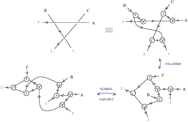
### Visual Description
## Diagram: Associative and Global Fan-Out Structures
### Overview
The image contains two interconnected diagrams labeled "CO-ASSOC" (left) and "GLOBAL FAN-OUT" (right), with bidirectional arrows between them. Both diagrams use nodes (A, B, C, ε, ε⁻¹) and directed arrows with numerical labels (1, 2, 3) to represent relationships.
### Components/Axes
- **Nodes**:
- **A, B, C**: Primary entities (likely variables or states).
- **ε, ε⁻¹**: Symbolic nodes (possibly representing errors, transformations, or inverse operations).
- **Arrows**:
- **Directional arrows** with numerical labels (1, 2, 3) indicate weighted or prioritized relationships.
- **Bidirectional arrow** labeled "GLOBAL FAN-OUT" connects the two diagrams.
- **Labels**:
- "CO-ASSOC" (top-left diagram).
- "GLOBAL FAN-OUT" (top-right diagram).
- Numerical labels (1, 2, 3) on arrows.
### Detailed Analysis
#### CO-ASSOC Diagram (Left)
- **Structure**:
- Arrows from **B → A** (labeled 3) and **C → A** (labeled 2) converge on **A**.
- A bidirectional arrow between **B** and **C** (labeled 1).
- Arrows from **A → ε** and **ε → C** suggest a feedback loop.
- **Flow**:
- Primary flow from **B** and **C** to **A**, with secondary interactions between **B** and **C**.
#### GLOBAL FAN-OUT Diagram (Right)
- **Structure**:
- Arrows from **B → ε**, **ε → A**, and **C → A** (labeled 2, 3).
- A loop between **ε** and **B** (labeled 1).
- Arrows from **A → ε** and **ε → C** mirror the CO-ASSOC diagram.
- **Flow**:
- Distributed connections from **B** and **C** to **A** via **ε**, with a feedback loop between **ε** and **B**.
#### Bidirectional Connection
- The "GLOBAL FAN-OUT" arrow links the two diagrams, implying a systemic relationship between associative (CO-ASSOC) and distributed (GLOBAL FAN-OUT) structures.
### Key Observations
1. **Numerical Weights**:
- **CO-ASSOC**: Stronger influence from **B → A** (3) than **C → A** (2).
- **GLOBAL FAN-OUT**: Equal weighting (2, 3) for **B → ε** and **C → A**.
2. **Feedback Loops**:
- Both diagrams include cycles (e.g., **A → ε → C** and **ε → B → ε**).
3. **Symmetry**:
- Mirrored structures in node connections (e.g., **B → A** in CO-ASSOC vs. **B → ε → A** in GLOBAL FAN-OUT).
### Interpretation
- **CO-ASSOC** represents a localized, associative system where **B** and **C** directly influence **A**, with a weaker interaction between **B** and **C**.
- **GLOBAL FAN-OUT** depicts a distributed system where **B** and **C** influence **A** indirectly via **ε**, with a feedback mechanism between **ε** and **B**.
- The bidirectional arrow suggests that the associative and global structures are interdependent, possibly modeling a system where local interactions (CO-ASSOC) and global distributions (GLOBAL FAN-OUT) coexist and influence each other.
- The numerical labels (1, 2, 3) may indicate priority, frequency, or strength of relationships, though their exact meaning depends on the system’s context (e.g., probabilistic weights, resource allocation).
## Notes
- No numerical data tables or heatmaps are present; the focus is on structural relationships.
- The diagrams likely model a theoretical framework (e.g., network theory, system dynamics) rather than empirical data.
- The use of ε and ε⁻¹ suggests abstract or symbolic operations (e.g., error correction, inverse transformations).
</details>
The graph from the left lower side is formed by an approximate difference, a ¯ ε gate and several Υ gates. Therefore, if A , B , C are computable in the sense of definition 5.4 then the initial graph (the translation of the LHS of R3d with A , B , C grafted at the inputs) is computable too.
Graphic beta move as braiding. Let us now construct crossings, in the sense previously explained, from gates coming from lambda calculus.
<details>
<summary>Image 68 Details</summary>
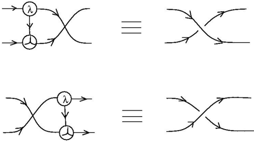
### Visual Description
## Diagram: Particle Interaction Schematics
### Overview
The image contains two schematic diagrams depicting particle interactions, connected by equivalence symbols (≡). Each diagram features directional arrows, labeled symbols (λ and a three-pronged circle), and no numerical data or explicit axis labels.
### Components/Axes
- **Symbols**:
- **λ (Lambda)**: Positioned at the top of the first diagram and the bottom of the second, likely representing a particle or interaction mediator.
- **Three-pronged circle**: Appears at the bottom of the first diagram and the top of the second, possibly denoting a particle decay or interaction vertex.
- **Arrows**: Indicate directional flow or causal relationships between components.
- **Equivalence Symbols (≡)**: Connect the two diagrams, suggesting they represent equivalent processes under specific conditions.
### Detailed Analysis
1. **Top Diagram**:
- Arrows flow from a three-pronged circle (bottom) to λ (top), then split into two divergent paths.
- The three-pronged circle has two incoming arrows and one outgoing arrow, while λ has one incoming and two outgoing arrows.
2. **Bottom Diagram**:
- Arrows flow from λ (top) to a three-pronged circle (bottom), with λ receiving one incoming arrow and emitting two outgoing arrows.
- The three-pronged circle receives two incoming arrows and emits one outgoing arrow.
3. **Equivalence**:
- The ≡ symbols imply the two diagrams are interchangeable or represent dual perspectives of the same interaction.
### Key Observations
- **Reversibility**: The diagrams are mirror images in terms of component placement (λ and three-pronged circle swap positions).
- **Conservation of Flow**: In both diagrams, the total number of incoming/outgoing arrows at each symbol matches, suggesting conservation laws (e.g., charge, momentum).
- **No Numerical Data**: No scales, units, or quantitative values are present.
### Interpretation
The diagrams likely represent particle physics processes, such as decay or scattering events. The equivalence (≡) suggests these are dual descriptions of the same phenomenon, possibly under Lorentz symmetry or charge conjugation. The three-pronged circle may symbolize a particle decaying into three components (e.g., a boson splitting into fermions), while λ could represent a mediator particle (e.g., a photon or gluon). The absence of numerical data implies this is a conceptual illustration rather than an empirical dataset.
**Note**: No textual labels, legends, or axis markers are present beyond the symbols λ and the three-pronged circle. The diagrams rely on symbolic representation rather than quantitative data.
</details>
As previously, we define translations of (locally planar) tangle diagrams into graphs in GRAPH . The class of locally planar tangle diagrams is out in a one-to one correspondence with a class of graphs in GRAPH , let us call this class λ -TANGLE .
We could proceed in the inverse direction, namely consider the class of graphs λ -TANGLE , along with the moves: graphic beta move and elimination of loops. Then we make the (inverse) translation of graphs in λ -TANGLE into locally planar tangle diagrams and the (inverse) translation of the graphic beta move and the elimination of loops. The following proposition explains what we obtain.
Proposition 6.2 The class of graphs λ -TANGLE is closed with respect to the application of the graphic beta move and of the elimination of loops. The translations of the graphic beta and elimination of loops moves are the following SPLICE 1, 2 (translation of the graphic beta move) and LOOP 1, 2 (translation of the elimination of loops) moves.
Proof. The proposition becomes obvious if we find the translation of the graphic beta move. There is one translation for each crossing. (Likewise, there are two translations for elimination of loops, depending on the orientation of the loop which is added/erased.)
<details>
<summary>Image 69 Details</summary>
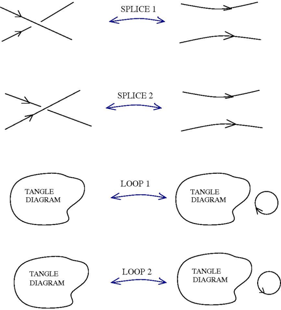
### Visual Description
## Flowchart: Tangle Diagrams and Transformations
### Overview
The image depicts a flowchart illustrating transformations between tangle diagrams and their simplified or modified forms. It includes labeled components ("SPLICE 1", "SPLICE 2", "LOOP 1", "LOOP 2") and directional arrows indicating processes.
### Components/Axes
- **Labels**:
- "SPLICE 1" and "SPLICE 2" (top section).
- "LOOP 1" and "LOOP 2" (bottom section).
- "TANGLE DIAGRAM" (input for both loops).
- **Arrows**:
- Blue bidirectional arrows between "TANGLE DIAGRAM" and "LOOP 1"/"LOOP 2".
- Unidirectional arrows within "SPLICE 1" and "SPLICE 2" (e.g., crossing lines transforming into parallel lines).
- **Diagrams**:
- "TANGLE DIAGRAM" (left side, abstract knot-like structure).
- "LOOP 1" and "LOOP 2" (right side, with "LOOP 2" containing an additional circular loop).
### Detailed Analysis
1. **SPLICE 1**:
- Two crossing lines (arrows) transform into two parallel lines via a splice operation.
- Arrows indicate the direction of simplification.
2. **SPLICE 2**:
- Similar to SPLICE 1 but with a different crossing configuration.
- Resulting parallel lines are oriented differently (e.g., upward vs. downward).
3. **LOOP 1**:
- A tangle diagram (input) transforms into a single-loop structure.
- Arrows suggest the process of closing the tangle into a loop.
4. **LOOP 2**:
- Similar to LOOP 1 but includes an additional circular loop appended to the primary loop.
- The extra loop is drawn separately but connected to the main loop.
### Key Observations
- **Simplification vs. Complexity**:
- Splices reduce complexity (crossing lines → parallel lines).
- Loops increase complexity by forming closed structures.
- **Asymmetry in LOOP 2**:
- The additional loop in LOOP 2 is distinct from LOOP 1, suggesting a secondary transformation step.
- **Directionality**:
- Arrows in splices point toward parallel lines, while loop arrows point from tangle diagrams to their looped forms.
### Interpretation
The diagram likely represents a mathematical or topological process where tangle diagrams (complex knot-like structures) are simplified via splicing or modified into loops. The asymmetry in LOOP 2 implies a hierarchical or multi-step transformation, where an initial loop is further elaborated. This could model concepts in knot theory, polymer chemistry, or network simplification algorithms. The absence of numerical data suggests a focus on structural relationships rather than quantitative analysis.
</details>
<details>
<summary>Image 70 Details</summary>
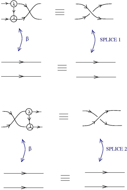
### Visual Description
## Diagram: Process Flow with Splicing and Feedback Loops
### Overview
The image depicts two equivalent process flow diagrams connected by equivalence symbols (≡). Each diagram illustrates a sequence of interactions involving branching, merging, and feedback loops, labeled with symbols (λ, β) and annotations ("SPLICE 1", "SPLICE 2"). The diagrams emphasize directional flow (arrows) and equivalence between transformations.
---
### Components/Axes
1. **Primary Elements**:
- **Arrows**: Indicate directional flow (left-to-right, upward/downward loops).
- **Circles with Symbols**:
- **λ (Lambda)**: Appears in two nodes, likely representing input or transformation points.
- **Three-way Junction**: A node with three outgoing paths, suggesting decision or merging logic.
- **β (Beta)**: Circular arrows below each diagram, representing feedback loops.
- **SPLICE 1/SPLICE 2**: Labels above the right-side diagrams, indicating distinct output paths.
2. **Equivalence Symbols (≡)**: Positioned between the left and right diagrams, denoting equivalence of processes.
3. **Spatial Layout**:
- **Top Row**: Left diagram (λ → three-way junction → λ) ≡ Right diagram (branching/merging arrows).
- **Bottom Row**: Left diagram (λ → three-way junction → λ) ≡ Right diagram (branching/merging arrows).
- **Feedback Loops (β)**: Positioned below each main diagram, looping vertically.
---
### Detailed Analysis
1. **Top Diagram**:
- **Left Side**:
- Input (λ) enters a three-way junction.
- Two paths merge into a single output (λ).
- **Right Side**:
- Two parallel input streams converge into a single output stream.
- **Equivalence**: The left and right diagrams represent the same process via different visual abstractions.
2. **Bottom Diagram**:
- **Left Side**:
- Input (λ) enters a three-way junction.
- Two paths split into separate outputs (λ).
- **Right Side**:
- A single input stream splits into two parallel outputs.
- **Equivalence**: Mirrors the top diagram’s logic but with inverted flow (splitting vs. merging).
3. **Feedback Loops (β)**:
- Circular arrows below each diagram suggest iterative processes or cyclical dependencies.
---
### Key Observations
- **Symmetry**: Both diagrams exhibit mirrored logic (splitting/merging) with equivalence.
- **Symbol Consistency**: λ appears in input/output nodes, while β governs feedback.
- **No Numerical Data**: The diagrams are conceptual, lacking quantitative values or scales.
---
### Interpretation
The diagrams likely represent **process equivalence in a system** (e.g., physics, engineering, or computer science). The λ symbols may denote inputs/outputs, while the three-way junction and β loops imply decision points and iterative feedback. The "SPLICE" labels suggest discrete output paths (SPLICE 1/2) resulting from the process. The equivalence symbols (≡) emphasize that the left and right diagrams are functionally identical despite differing visual representations. This could model scenarios like signal processing, data routing, or theoretical transformations where multiple pathways yield the same outcome.
</details>
The following theorem clarifies which are the oriented Reidemeister moves which can be expressed as sequences of graphic lambda calculus moves applied to graphs in λ -TANGLE . Among these moves, some are more powerful than others, as witnessed by the following
Theorem 6.3 All the translations of the oriented Reidemeister move into moves between graphs in λ -TANGLE , excepting R2c, R2d, R3a, R3h, can be realized as sequences of graphic beta moves and elimination of loops. Moreover, the translations of moves R2c, R2d, R3a, R3h are equivalent up to graphic beta moves and elimination of loops (i.e. any of these moves, together with the graphic beta move and elimination of loops, generates the other moves from this list).
Proof. It is easy, but tedious, to verify that all the mentioned moves can be realized as sequences of SPLICE and LOOP moves. It is as well easy to verify that the moves R2c, R2d, R3a, R3h are equivalent up to SPLICE and LOOP moves. It is not obvious that the moves R2c, R2d, R3a, R3h can't be realized as a sequence of SPLICE and LOOP moves. In order to do this, we prove that R2d can't be generated by SPLICE and LOOP. Thanks are due to Peter Kravchuk for the idea of the proof, given in an answer to a question I asked on mathoverflow [7], where I described the moves SPLICE and LOOP.
To any locally planar tangle diagram A associate it's reduced diagram R(A), which is obtained by the following procedure: first use SPLICE 1,2 from left to right for all crossings, then use LOOP 1,2 from right to left in order to eliminate all loops which are present at this stage. Notice that:
-the order of application of the SPLICE moves does not matter, because they are applied
only once per crossing. There is a finite number of splices, equal to the number of crossings. Define the bag of splices SPLICE(A) to be the set of SPLICE moves applied.
- -The same is true for the order of eliminations of loops by LOOP 1, 2. There is a finite number of loop eliminations, because the number of loops (at this stage) cannot be bigger than the number of edges of the initial diagram. Define the bag of loops LOOP(A) to be the set of all loops which are present after all splices are done.
Let us now check that the reduced diagram does not change if one of the 4 moves is applied to the initial diagram.
Apply a SPLICE 1,2 move to the initial diagram A, from left to right, and get B. Then SPLICE(B) is what is left in the bag SPLICE(A) after taking out the respective splice. Also LOOP(B) = LOOP(A) because of the definition of bags of loops. Therefore R(A) = R(B).
Apply a SPLICE 1, 2 from right to left to A and get B. Then R(A) = R(B) by the same proof, with A, B switching places.
Apply a LOOP1, 2 from left to right to A and get B. The new loop introduced in the diagram does not participate to any crossing (therefore SPLICE(A) = SPLICE(B)), so we find it in the bag of loops of B, which is made by all the elements of LOOP(A) and this new loop. Therefore R(A) = R(B). Same goes for LOOP1, 2 applied from right to left.
Finally, remark that the reduced diagram of the LHS of the move R2d is different than the reduced diagram of the RHS of the move R2d, therefore the move R2d cannot be achieved with a sequence of splices and loops addition/elimination.
## References
- [1] A. Bella¨ ıche, The tangent space in sub-Riemannian geometry, in: Sub-Riemannian Geometry, A. Bella¨ ıche, J.-J. Risler eds., Progress in Mathematics , 144 , Birkh¨ auser, (1996), 4-78
- [2] M. Buliga, Dilatation structures I. Fundamentals, J. Gen. Lie Theory Appl. , 1 (2007), 2, 65-95. arXiv:math/0608536
- [3] M. Buliga, Emergent algebras, arXiv:0907.1520
- [4] M. Buliga, Braided spaces with dilations and sub-riemannian symmetric spaces, in: Geometry. Exploratory Workshop on Differential Geometry and its Applications, eds. D. Andrica, S. Moroianu, Cluj-Napoca 2011, 21-35, arXiv:1005.5031
- [5] M. Buliga, λ -Scale, a lambda calculus for spaces with dilations, arXiv:1205.0139
- [6] M. Buliga, Computing with space: a tangle formalism for chora and difference , arXiv:1103.6007
- [7] MBuliga, Oriented Reidemeister move R2d by splices and loop adding/erasing?, mathoverflow question (version: 2013-04-23)
- [8] W. Citrin, R. Hall, B. Zorn. Programming with visual expressions. Proceedings of the 11th International IEEE Symposium on Visual Languages, 1995, pp 294-301
- [9] M. Erwig, Abstract syntax and semantics of visual languages, Journal of Visual Languages and Computing 9 (1998), No. 5, 461-483.
- [10] R. Fenn, C. Rourke, Racks and Links in codimension two, J. Knot Theory Ramifications , 1 (1992), no. 4, 343-406
- [11] M. Gromov, Carnot-Carath´ eodory spaces seen from within, in the book: SubRiemannian Geometry, A. Bella¨ ıche, J.-J. Risler eds., Progress in Mathematics , 144 , Birkh¨ auser, (1996), 79-323.
- [12] H. Gl¨ ockner, Contractible Lie groups over local fields, Math. Z. 260 (2008), 889-904, arXiv:0704.3737
- [13] D. Joyce, A classifying invariant of knots; the knot quandle, J. Pure Appl. Alg. , 23 (1982), 37-65
- [14] L. Kauffman, Knot logic. Knots and applications, 1110, Ser. Knots Everything, 6, World Sci. Publ., River Edge, NJ, 1995
- [15] David C Keenan. To Dissect a Mockingbird: A Graphical Notation for the Lambda Calculus with Animated Reduction, 2001. http://dkeenan.com/Lambda/
- [16] J.J. Koenderink, The brain a geometry engine, Psychological Research , 52 (1990), no. 2-3, 122-127
- [17] L.G. Meredith, D.F. Snyder, Knots as processes: a new kind of invariant, arXiv:1009.2107
- [18] P. Pansu, M´ etriques de Carnot-Carath´ eodory et quasi-isom´ etries des espaces sym´ etriques de rang un, Ann. of Math., (2) 129 , (1989), 1-60.
- [19] M. Polyak, Minimal generating sets of Reidemeister moves, arXiv:0908.3127
- [20] E. Siebert, Contractive automorphisms on locally compact groups, Math. Z. 191 1986, Issue 1, pp 73-90.
- [21] D.P. Thurston, The algebra of knotted trivalent graphs and Turaevs shadow world arXiv:math/0311458