1306.1461

# The GTZAN dataset: Its contents, its faults, their effects on evaluation, and its future use **Authors**: Bob L. Sturm ## The GTZAN dataset: Its contents, its faults, their effects on evaluation, and its future use Bob L. Sturm ∗ November 27, 2024 ## Abstract The GTZAN dataset appears in at least 100 published works, and is the most-used public dataset for evaluation in machine listening research for music genre recognition (MGR). Our recent work, however, shows GTZAN has several faults (repetitions, mislabelings, and distortions), which challenge the interpretability of any result derived using it. In this article, we disprove the claims that all MGR systems are affected in the same ways by these faults, and that the performances of MGR systems in GTZAN are still meaningfully comparable since they all face the same faults. We identify and analyze the contents of GTZAN , and provide a catalog of its faults. We review how GTZAN has been used in MGR research, and find few indications that its faults have been known and considered. Finally, we rigorously study the effects of its faults on evaluating five different MGR systems. The lesson is not to banish GTZAN , but to use it with consideration of its contents. ## 1 Introduction Our recent review of over 467 published works in music genre recognition (MGR) [1] shows that the most-used public dataset is GTZAN , 1 appearing in the evaluations of 100 works [2-101]. GTZAN is composed of 1,000 half-minute music audio excerpts singly labeled in ten categories [92, 93]; and though its use is so widespread, it has always been missing metadata identifying its contents. In fact, GTZAN was not expressly created for MGR, 2 but its availability has made it a benchmark dataset, and thus a measuring stick for comparing MGR systems, ∗ B. L. Sturm is with the Audio Analysis Lab, AD:MT, Aalborg University Copenhagen, A.C. Meyers Vænge 15, DK-2450 Copenhagen, Denmark, (+45) 99407633, fax: (+45) 44651800, email: bst@create.aau.dk. He is supported in part by Independent Postdoc Grant 11-105218 from Det Frie Forskningsr˚ ad; the Danish Council for Strategic Research of the Danish Agency for Science Technology and Innovation in project CoSound, case no. 11-115328. 1 http://marsyas.info/download/data\_sets 2 Personal communication with G. Tzanetakis e.g., [102]. However, few researchers have ever listened to and critically evaluated the contents of GTZAN , and thus its faults remained undiscovered since its creation in 2002. Our previous work [103] provides the first metadata for GTZAN , and identifies several faults in its integrity: repetitions, mislabelings, and distortions. In that paper, however, we do not find the extent to which GTZAN appears in the literature, and do not survey the ways in which it has been used. We do not measure how its faults affect evaluation in MGR; and, furthermore, we do not provide any recommendations for its future use. This article rigorously addresses all of these, significantly extending our analysis of GTZAN in several practical ways. Our work not only illuminates results reported by a significant amount of work, but also provides a critical piece to address the non-trivial problems associated with evaluating music machine listening systems in valid ways [1,83,84,103-105]. As a brief menu of our main results, the most significant one is that we disprove the claims: 'all MGR systems are affected in the same ways by the faults in GTZAN ', and 'the performances of all MGR systems in GTZAN , working with the same data and faults, are still meaningfully comparable.' This shows that, for the 100 works performing evaluation in GTZAN [2-101], one cannot make any meaningful conclusion about which system is better than another for reproducing the labels of GTZAN , let alone which is even addressing the principal goals of MGR [105]. We find that of these 100 works, more appear in 2010 - 2012 than in the eight years after its creation. We find only five works (outside our own [83-86], and [99] which references [103]) that indicate someone has listened to some of GTZAN . Of these, one work explicitly endorses its integrity for MGR evaluation, while four allude to some problems. We find no work (outside our own [83-86]) that explicitly considers the musical content of GTZAN in evaluation. The lesson of this article is not that GTZAN should be banished, but that it must be used with consideration of its contents . Its faults, which are representative of data in the real-world, can in fact be used in the service of evaluation [84], no matter if it is MGR, or other music machine listening tasks. In the next subsection, we enumerate our contributions, and then explicitly state delimitations of this article. We then address several criticisms that have been raised in reviews of versions of this work. In the second section, we extend our previous analysis of GTZAN [103]. In the third section, we comprehensively survey how GTZAN has been used. In the fourth section, we test the effects of its faults on the evaluation of several categorically different and state-of-the-art MGR systems. Finally, we conclude by describing how GTZAN can be useful to future research. We make available on-line the MATLAB code to reproduce all results and figures, as well as the metadata for GTZAN : http://imi.aau.dk/ ~ bst . ## 1.1 Contributions 1. We evaluate for several MGR systems the effects of the faults in GTZAN when evaluating performance, and falsify the claims: 'all MGR systems are affected in the same ways by the faults in GTZAN ', and 'the performances - of all MGR systems in GTZAN , working with the same data and faults, are still meaningfully comparable.' 2. We estimate upper bounds for several figures of merit for the 'perfect' MGR system evaluated using GTZAN . 3. We significantly extend our prior analysis of GTZAN [103]: we create metadata for 110 more excerpts; we devise an approach to analyze the composition and meaning of the categories of GTZAN ; and we formally define and identify mislabelings. 4. We demonstrate how GTZAN can be useful for future research in MGR, audio similarity, autotagging, etc. 5. We confirm the prediction of Seyerlehner [75, 76] that GTZAN has a large amount of artist repetition; we measure for the first time for GTZAN the effect of this on MGR evaluation. 6. We provide a comprehensive survey of how GTZAN has been used, which ties together 100 published works that use GTZAN for evaluation, and thus are affected by its faults. ## 1.2 Delimitations This article is concerned only with GTZAN : its composition and faults; its historical and contemporary use for evaluating MGR systems; the effects of its faults on evaluating MGR systems; and how to use it with consideration of its problems. This article is not concerned with other public datasets, which may or may not suffer from the same faults as GTZAN , but which have certainly been used in fewer published works than GTZAN [1]. This article is not concerned with the validity, well-posedness, value, usefulness, or applicability of MGR; or whether MGR is 'replaced by,' or used in the service of, e.g., music similarity, autotagging, or the like. It is not concerned with making general conclusions about or criticisms of MGR or evaluation in MGR, which are comprehensively addressed in other works, e.g., [1, 83, 84, 105-109]. Finally, it is not concerned with how, or even whether it is possible, to create faultless datasets for MGR, music similarity, autotagging, and the like. 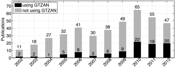## 1.3 Criticisms A variety of criticisms have been raised in reviews of this work. First, its usefulness has been challenged: 'recent publications are no longer using GTZAN '; or, 'it is already a commonly accepted opinion that the GTZAN dataset should be discarded'; or, 'better datasets are available.' The fact is, of all datasets that are publicly available, GTZAN is the one appearing most in published MGR work [1]. The fact is, more papers use GTZAN in the past three years than in the first eight years of its existence (Fig. 3), and none of them mention a 'common opinion' that GTZAN should be discarded. Even with its faults, the fact is that GTZAN can be useful [84, 86], and there is no reason to discard it. Our work provides novel insights and perspectives essential for interpreting all published results that use GTZAN , in the past and in the future, and ways for better scientific evaluation using it. These facts provide strong argumentation for the publication and preservation of this work in an archival form. One might challenge the aims of published work that uses GTZAN : 'to some extent genre classification has been replaced by the more general problem of automatic tagging'; or, 'genre classification is now critically seen even by the person who compiled GTZAN (personal communication with Tzanetakis).' The fact is, researchers have published and still are publishing a large number of works in MGR that use GTZAN . One might argue, 'this article only touches the possibility of a critique of genre classification'; or, 'it misses the valuable chance to criticize the simplistic and superficial approach to music that governs most of these publications'; or, 'it falls short of providing a more rigorous questioning of MGR evaluation and a more general evaluation that goes beyond the GTZAN dataset.' Such aspects, however, are outside the scope of this article delimited above, but are thoroughly addressed by other work, e.g., [1,83,84,105,107-109]. ## 2 Analysis of GTZAN To analyze GTZAN , we first identify its excerpts, see how artists compose each category, and survey the ways people describe the music. Finally, we delimit and identify three kinds of faults in the dataset: repetitions, mislabelings, and distortions (summarized in Table 2). ## 2.1 Identifying excerpts We use the Echo Nest Musical Fingerprinter (ENMFP) 3 to generate a fingerprint of every excerpt in GTZAN and to query the Echo Nest database having over 30,000,000 songs. The second column of Table 1 shows that this identifies only 60.6% of the excerpts. We correct titles and artists as much as possible, and find four misidentifications. We then manually identify 313 of the remaining excerpts. The third column of Table 1 shows that we miss the metadata of only 81 excerpts. With this, we can now bound the number of artists in GTZAN -which has been stated to be unknown, e.g., [75, 76]. Assuming each of the unidentified excerpts come from different artists than those we have identified, the total number of artists represented in the excerpts of GTZAN cannot be larger than 329. If all unlabeled excerpts are from the same artists we have identified, then the smallest it can be is 248. 3 http://developer.echonest.com Table 1: For each category of GTZAN : number of excerpts we identify by fingerprint (ENMFP); then searching manually (self); number of songs in last.fm (and number of tags having 'count' larger than 0); for tracks not found, number of artists in last.fm (and number of tags having 'count' larger than 0). Retrieved Dec. 25, 2012, 21h. | | | | last.fm | last.fm | |-----------|-------|-------|-----------------|-------------------| | Label | ENMFP | self | song (no. tags) | artist (no. tags) | | Blues | 63 | 100 | 75 (2904) | 25 (2061) | | Classical | 63 | 97 | 12 (400) | 85 (4044) | | Country | 54 | 95 | 81 (2475) | 13 (585) | | Disco | 52 | 90 | 82 (5041) | 8 (194) | | Hip hop | 64 | 96 | 90 (6289) | 5 (263) | | Jazz | 65 | 80 | 54 (1127) | 26 (2102) | | Metal | 65 | 83 | 73 (5579) | 10 (786) | | Pop | 59 | 96 | 89 (7173) | 7 (665) | | Reggae | 54 | 82 | 73 (4352) | 9 (616) | | Rock | 67 | 100 | 99 (7227) | 1 (100) | | Total | 60.6% | 91.9% | 72.8% (42567) | 18.9% (11416) | ## 2.2 Describing excerpts and categories To survey the ways people describe the music or artist of each excerpt, we query the application programming interface provided by last.fm , and retrieve the 'tags' users of the service apply to the songs or artists in GTZAN . A tag is a word or phrase a person uses to describe an artist, or a song, in order to make their music collection more useful for them. On last.fm , tags are most often genre labels ('Blues') [110], but they can also describe instrumentation ('female vocalists'), tempo ('120 bpm'), mood ('happy'), how the music is used ('exercise'), lyrics ('fa la la la la'), reproduce the band name ('The Rolling Stones'), or something else ('favorite song of all time') [111]. We assume the tags users give to a song or artist would also be given to the excerpt in GTZAN . Tags from last.fm have been used in other work, e.g., [112,113]. The collection of these tags is of course far from being controlled; but an aspect that helps strengthen their use is that last.fm provides a 'count' for each one: a normalized quantity such that 100 means the tag is applied by most listeners, and 0 means the tag is applied by the fewest. We keep only those tags with counts greater than 0. The fourth column of Table 1 shows the number of tracks we identify that have tags in last.fm , and the number of tags with non-zero count. When we do not find tags for a song, we get the tags applied to the artist. For instance, though we identify all 100 excerpts in Blues, only 75 of the songs are tagged. Of these, we get 2,904 tags with non-zero counts. For the remaining 25 songs, we retrieve 2,061 tags from the tags given to the artists. 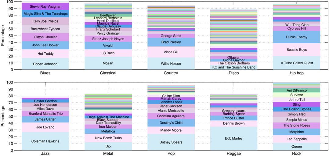Figure 1: Artist composition of each GTZAN category. We do not include unidentified excerpts. <details> <summary>Image 1 Details</summary>  ### Visual Description ## Stacked Bar Chart: Artist Prominence by Music Genre ### Overview The image is a dual-section stacked bar chart comparing the relative prominence of artists across 10 music genres. Each bar represents a genre, divided into colored segments corresponding to individual artists. The y-axis shows percentage contribution (0-100%), while the x-axis categorizes genres into two groups: "Traditional/Classic" (Blues, Classical, Country, Disco, Hip hop) and "Modern/Contemporary" (Jazz, Metal, Pop, Reggae, Rock). The right-side legend maps colors to specific artists. ### Components/Axes - **X-axis**: - **Top Section**: Blues, Classical, Country, Disco, Hip hop - **Bottom Section**: Jazz, Metal, Pop, Reggae, Rock - **Y-axis**: Percentage scale (0-100%) with no intermediate markers - **Legend**: Right-aligned, color-coded artist names (e.g., purple = Stevie Ray Vaughan, blue = Bob Marley) - **Bars**: Stacked vertically, with each segment representing an artist's relative prominence ### Detailed Analysis #### Traditional/Classic Genres 1. **Blues** (Leftmost bar): - Stevie Ray Vaughan (purple, ~85%) - Magic Slim & The Teardrops (dark blue, ~75%) - Kelly Joe Phelps (pink, ~65%) - Buckwheat Zydeco (orange, ~55%) - Clifton Chenier (light blue, ~45%) - John Lee Hooker (cyan, ~35%) - Hot Toddy (magenta, ~25%) - Robert Johnson (lavender, ~15%) 2. **Classical** (Second bar): - Beethoven (green, ~90%) - Leonard Bernstein (teal, ~80%) - Mozart (blue, ~70%) - JS Bach (purple, ~60%) - Vivaldi (orange, ~50%) - Franz Joseph Haydn (pink, ~40%) - Claude Debussy (cyan, ~30%) - Percy Granger (magenta, ~20%) 3. **Country** (Third bar): - Willie Nelson (green, ~85%) - George Strait (teal, ~75%) - Brad Paisley (blue, ~65%) - Vince Gill (purple, ~55%) - K.C. and The Sunshine Band (orange, ~45%) - The Gibson Brothers (pink, ~35%) - Ottway (cyan, ~25%) - Gloria Gaynor (magenta, ~15%) 4. **Disco** (Fourth bar): - KC and The Sunshine Band (green, ~90%) - Gloria Gaynor (teal, ~80%) - The Gibson Brothers (blue, ~70%) - Ottawan (purple, ~60%) - Survivor (orange, ~50%) - Public Enemy (pink, ~40%) - Wu-Tang Clan (cyan, ~30%) - Cypress Hill (magenta, ~20%) 5. **Hip hop** (Fifth bar): - Wu-Tang Clan (green, ~85%) - Cypress Hill (teal, ~75%) - Public Enemy (blue, ~65%) - Beastie Boys (purple, ~55%) - A Tribe Called Quest (orange, ~45%) - Survivor (pink, ~35%) - Jehro Tull (cyan, ~25%) - Sting (magenta, ~15%) #### Modern/Contemporary Genres 1. **Jazz** (Leftmost bar in bottom section): - Coleman Hawkins (green, ~90%) - Joe Lovano (teal, ~80%) - Branford Marsalis Trio (blue, ~70%) - Miles Davis (purple, ~60%) - Joe Henderson (orange, ~50%) - Dexter Gordon (pink, ~40%) - James Carter (cyan, ~30%) - Rage Against The Machine (magenta, ~20%) 2. **Metal** (Second bar): - Metallica (green, ~90%) - Iron Maiden (teal, ~80%) - New Bomb Turks (blue, ~70%) - Dio (purple, ~60%) - Rage Against The Machine (orange, ~50%) - Dark Tranquillity (pink, ~40%) - Black Sabbath (cyan, ~30%) - Moby (magenta, ~20%) 3. **Pop** (Third bar): - Celine Dion (green, ~90%) - Mariah Carey (teal, ~80%) - Janet Jackson (blue, ~70%) - Alanis Morissette (purple, ~60%) - Christina Aguilera (orange, ~50%) - Mandy Moore (pink, ~40%) - Britney Spears (cyan, ~30%) - The Stone Roses (magenta, ~20%) 4. **Reggae** (Fourth bar): - Bob Marley (green, ~95%) - Dennis Brown (teal, ~85%) - Gregory Isaacs (blue, ~75%) - Burning Spear (purple, ~65%) - Prince Buster (orange, ~55%) - Simple Minds (pink, ~45%) - The Stone Roses (cyan, ~35%) - The Rolling Stones (magenta, ~25%) 5. **Rock** (Rightmost bar): - Queen (green, ~90%) - Led Zeppelin (teal, ~80%) - The Rolling Stones (blue, ~70%) - Simple Minds (purple, ~60%) - The Stone Roses (orange, ~50%) - Sting (pink, ~40%) - Simple Red (cyan, ~30%) - Ani Difranco (magenta, ~20%) ### Key Observations 1. **Dominant Artists**: - Reggae: Bob Marley occupies ~95% of the bar, dwarfing others. - Hip hop: Wu-Tang Clan (~85%) and Cypress Hill (~75%) dominate. - Classical: Beethoven (~90%) and Bernstein (~80%) lead. 2. **Genre Contrasts**: - **Classical** and **Disco** show tightly packed segments (narrower range of prominence). - **Jazz** and **Metal** have more pronounced hierarchies (e.g., Coleman Hawkins at ~90% vs. Rage Against The Machine at ~20% in Jazz). 3. **Anomalies**: - **Disco**: Public Enemy (~40%) and Wu-Tang Clan (~30%) appear in a genre they did not originate, suggesting cross-genre influence. - **Hip hop**: Beastie Boys (~55%) and A Tribe Called Quest (~45%) are lower than expected for pioneers. ### Interpretation The chart visualizes the **relative cultural weight** of artists within genres, likely reflecting popularity, influence, or historical significance. Dominant figures like Bob Marley (Reggae) and Beethoven (Classical) anchor their genres, while outliers like Public Enemy in Disco suggest cross-genre impact. The stacked format emphasizes **hierarchical prominence**, with top segments representing the most iconic artists. Modern genres (Jazz, Metal) show sharper divisions between top and lesser-known artists compared to traditional genres, where mid-tier artists (e.g., Franz Joseph Haydn in Classical) retain moderate prominence. This could reflect evolving genre dynamics, where contemporary styles fragment influence more rapidly than established ones. 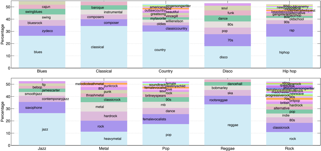</details> Figure 2: Top tags of each GTZAN category. We do not include unidentified excerpts. <details> <summary>Image 2 Details</summary>  ### Visual Description ## Stacked Bar Chart: Genre and Sub-Genre Distribution ### Overview The image is a stacked bar chart divided into two sections: **Genres** (top) and **Sub-Genres** (bottom). Each bar represents a genre or sub-genre, with segments colored to indicate specific terms. The y-axis is labeled "Percentage" (0–50), and the x-axis lists genres (e.g., Blues, Classical, Country, Disco, Hip hop) and sub-genres (e.g., Jazz, Metal, Pop, Reggae, Rock). A legend on the right maps colors to terms. --- ### Components/Axes - **X-Axis**: - Top section: Genres (Blues, Classical, Country, Disco, Hip hop). - Bottom section: Sub-Genres (Jazz, Metal, Pop, Reggae, Rock). - **Y-Axis**: - Labeled "Percentage" (0–50). - **Legend**: - Located on the right, with colors corresponding to terms (e.g., "blues" in light blue, "jazz" in dark blue, "metal" in gray, etc.). - **Bars**: - Stacked vertically, with each segment representing a term. Labels are placed above or below segments. --- ### Detailed Analysis #### Genres Section (Top) 1. **Blues**: - Largest segment: "blues" (light blue, ~30%). - Other segments: "zydeco" (purple, ~10%), "swing" (green, ~5%), "cajun" (pink, ~5%), "bluesrock" (pink, ~5%). 2. **Classical**: - Largest segment: "classical" (light blue, ~40%). - Other segments: "composer" (purple, ~10%), "instrumental" (green, ~5%), "baroque" (pink, ~5%). 3. **Country**: - Largest segment: "country" (light blue, ~40%). - Other segments: "folk" (purple, ~10%), "outlawcountry" (green, ~5%), "americansongwriter" (pink, ~5%). 4. **Disco**: - Largest segment: "disco" (light blue, ~30%). - Other segments: "70s" (purple, ~10%), "dance" (green, ~5%), "80s" (pink, ~5%). 5. **Hip hop**: - Largest segment: "hip hop" (light blue, ~30%). - Other segments: "rap" (purple, ~10%), "rnb" (green, ~5%), "90s" (pink, ~5%). #### Sub-Genres Section (Bottom) 1. **Jazz**: - Largest segment: "jazz" (light blue, ~30%). - Other segments: "saxophone" (purple, ~10%), "contemporaryjazz" (green, ~5%), "smoothjazz" (pink, ~5%). 2. **Metal**: - Largest segment: "metal" (light blue, ~30%). - Other segments: "hardrock" (purple, ~10%), "thrashmetal" (green, ~5%), "80s" (pink, ~5%). 3. **Pop**: - Largest segment: "pop" (light blue, ~30%). - Other segments: "dance" (purple, ~10%), "femalevocalists" (green, ~5%), "90s" (pink, ~5%). 4. **Reggae**: - Largest segment: "reggae" (light blue, ~30%). - Other segments: "ska" (purple, ~10%), "rootsreggae" (green, ~5%), "80s" (pink, ~5%). 5. **Rock**: - Largest segment: "rock" (light blue, ~30%). - Other segments: "classicrock" (purple, ~10%), "hardrock" (green, ~5%), "80s" (pink, ~5%). --- ### Key Observations - **Dominance of Main Genres**: The primary genre term (e.g., "blues," "classical") occupies the largest portion of each bar, indicating its central role. - **Sub-Genre Diversity**: Sub-genres vary in size, with some (e.g., "jazz," "metal") having more distinct sub-categories than others. - **Temporal Labels**: Terms like "80s," "90s," and "disco" suggest historical or cultural influences. - **Color Consistency**: The legend colors match the segments exactly (e.g., "blues" is light blue, "jazz" is dark blue). --- ### Interpretation The chart illustrates the hierarchical structure of musical genres and sub-genres, emphasizing the dominance of core genres while highlighting their subdivisions. For example: - **Hip hop** and **Reggae** show strong ties to "rap" and "ska," respectively, reflecting their cultural roots. - **Pop** and **Jazz** include terms like "femalevocalists" and "saxophone," indicating stylistic or instrumental focuses. - The inclusion of "80s," "90s," and "disco" suggests a focus on historical or era-specific trends. This visualization could represent data from a music database, chart analysis, or cultural study, emphasizing how genres evolve and intersect. The consistent use of color and labeling ensures clarity, though the absence of numerical values for each segment limits precise quantification. </details> We devise the following novel approach to identify the top tags of a music excerpt. Let ω i be its i th tag, and c i be its count. Given the set of |I| tag-count pairs { ( w i , c i ) } i ∈I , we call the top tags of an excerpt T := { ( w j , c j ) } j ∈J⊆I those that contribute the majority of the total tag count, i.e., $$\sum _ { i \in J ^ { \prime } } 1 _ { i \in I } \sum _ { j \in J ^ { \prime } } c _ { i j } ( 1 )$$ For example, consider an excerpt has the set of tag-count pairs: { ('folk' , 11) , ('blues' , 100) , ('blues guitar' , 90) } . Its total tag count is 201, and so its top tags are 'blues' and 'blues guitar', which account for 94 . 6% = 100(100 + 90) / 201 of the total tag count. We argue that the top tags of an excerpt give a satisfactory description of music content since they are given by the majority of users who have tagged the piece of music. In our previous analysis of GTZAN [103], we assume that since there is a category named, e.g., 'Country,' then the content of those excerpts should possess typical and distinguishing characteristics of music using the country genre [114]: stringed instruments such as guitar, mandolin, banjo; emphasized 'twang' in playing and singing; lyrics about patriotism, hard work and hard times; and so on. This leads us to claim in [103] that at least seven excerpts are mislabeled 'Country' because they have few of these characteristics. In fact, we find other work that assumes the concepts of two music genre datasets overlap because they share the same labels, e.g., the taxonomies in [26,58]. We make no such assumption here, and instead consider a label of GTZAN to represent the set of top tags of the set of excerpts labeled so. To find the top tags of the set of excerpts with a label, we first construct for the set of tag-count pairs { ( w k , c k )) } k ∈K by summing the counts for all |K| unique tags of the identified excerpts. We then compute the normalized count of each tag: $$c ( w _ { k } ) := c _ { k } / \sum _ { k \in K } c _ { k }$$ and finally define the top tags of this category by (1). Figure 2 shows the top tags for each category, where we can see that most of the top tags are indicative of genre. Now, we can see how GTZAN Blues means more than the blues of, e.g., Robert Johnson and John Lee Hooker; and how GTZAN Disco is more broad than the dance music from the seventies [114,115]. ## 2.3 Identifying faults: Repetitions We consider four types of repetition, from high to low specificity: exact, recording, artist, and version. We define an exact repetition as when two excerpts are the same to such a degree that their time-frequency fingerprints are highly similar. To find exact repetitions, we implement a simplified version of the Shazam fingerprint [116], compare every pair of excerpts, and then listen to confirm. The second column of Table 2 shows these In total, we find 50 exact repetitions in GTZAN . We define a recording repetition as when two excerpts come from the same recording, but are not detected with fingerprinting. We find these by looking for artists and songs appearing multiple times in the metadata. To confirm, we listen to the excerpts. The second and third columns of Table 2 shows these. We find Pop has the most exact and recording repetitions (16): 'Lady Marmalade' sung by Christina Aguilera et al., as well as 'Bootylicious' by Destiny's Child, each appear four times. In total, we find 21 recording repetitions in GTZAN . We define artist repetition as excerpts performed by the same artist, which are easily found using the metadata. Table 2 shows how every category of GTZAN has artist repetition. We see the 100 excerpts in Blues come from only nine artists; and more than a third of the excerpts labeled Reggae come from Bob Marley. We define a version repetition as when two excerpts are of the same song but performed differently. This could be a studio version, a live version, performed by the same or different artists, or even a remix. We identify these with the metadata, and then confirming by listening. For instance, Classical 44 and 48 are from 'Rhapsody in Blue' by George Gershwin, but performed by different orchestras. Metal 33 is 'Enter Sandman' by Metallica, and Metal 74 is a parody. In total, we find 13 version repetitions in GTZAN . ## 2.4 Identifying faults: Mislabelings In [103], we consider two kinds of mislabelings: contentious and conspicuous. We based these upon non-concrete criteria formed loosely around musicological principles associated with the genre labels of GTZAN - which we have shown above are not indicative of the content of each category. Here, we formalize the identification of mislabeled excerpts by using the concept of top tags we develop above. Consider an excerpt with label g ∈ G has the set of tag-normalized count pairs X = { ( w i , ¯ c i ( w i )) } i ∈I . We know label r ∈ G has the set of top tag-normalized count pairs T r = { ( y j , ¯ d ( y j )) } j ∈J r . We define the r -label score of X $$C ( x , T _ { r } ) = \sum _ { i \in J _ { r } } ^ { c _ { i } } d _ { j } ( y _ { j } ) \sum _ { i \in I _ { r } } ^ { c _ { i } }$$ where δ y j ≡ w i = 1 if y j and w i are identical, or zero otherwise. Note, this compares all tags of an excerpt to only the top tags of label r . Now, if C ( X , T g ) is too small (the tags of the excerpt have too little in common with the top tags of its label), or if C ( X , T r ) is too large for an r = g (the tags of the excerpt have more in common with the top tags of another label), then we say the excerpt is mislabeled. Table 2: Repetitions, mislabelings and distortions in GTZAN . Excerpt numbers are in parentheses. | Label | Exact | Recording | Repetitions | Version | Mislabelings | Distortions | |-----------|-------------------------------------------------------------------------------------------------|-------------------------------------------------|------------------------------------------------------------------------------------------------------------------------------------------------------------------------------------------------------------------------------------------------------------------|-----------------------------------------------------|-----------------------------------------------------------------------------------------------------------------------------------------------------------------------------------------------------------------------------------------------------------------------------------------------------------------------------------------------------------------------------------------------------------------------------------------------------------------|--------------------------------------------------------------------| | Blues | | | Artist John Lee Hooker (0-11); Robert Johnson (12-28); Kelly Joe Phelps (29-39); Stevie Ray Vaughn (40- 49); Magic Slim (50-60); Clifton Chenier (61-72); Buckwheat Zydeco (73-84); Hot Toddy (85-97); Al- bert Collins (98, 99) | | | | | Classical | | (42,53) (51,80) | J. S. Bach (00-10); Mozart (11-29); Debussy (30-33); Ravel (34-37); Dutilleux (38-41); Schubert (63-67); Haydn (68-76); Grainger (82-88); Vivaldi (89-99); and others | (44,48) | | static (49) | | Country | | (08,51) (52,60) | Willie Nelson (19,26,65-80); Vince Gill (50-64); Brad Paisley (81-93); George Strait (94-99); and others | (46,47) | Wayne Toups & Zydecajun 'Johnnie Can't Dance' (39) | static dis- tortion (2) | | Disco | (50,51,70) (55,60,89) (71,74) (98,99) | (38,78) | Gloria Gaynor (1,21, 38,78); Ottawan (17,24,44,45); The Gibson Brothers (22,28,30,35,37); KC and The Sunshine Band (49-51,70,71,73,74); ABBA (67,68,72); and others | (66,69) | Billy Ocean 'Can You Feel It' (11); Clarence Carter 'Patches' (20); Latoya Jackson 'Playboy' (23), '(Baby) Do The Salsa' (26); The Sugarhill Gang 'Rapper's Delight' (27); Evelyn Thomas 'Heart- less' (29), Reflections (34) | clipping dis- tortion (63) | | Hip hop | (39,45) (76,78) | (01,42) (46,65) (47,67) (48,68) (49,69) (50,72) | Wu-Tang Clan (1,7,41,42); Beastie Boys (8-25); A Tribe Called Quest (46-51,62-75); Cypress Hill (55- 61); Public Enemy (81-98); and others | (02,32) | 3LW 'No More (Baby I'ma Do Right)' (26); Aaliyah 'Try Again' (29); Pink 'Can't Take Me Home' (31); Lauryn Hill 'Ex-Factor' (40) | clipping distortion (3,5); skip at start (38) | | Jazz | (33,51) (34,53) (35,55) (36,58) (37,60) (38,62) (39,65) (40,67) (42,68) (43,69) (44,70) (45,71) | | James Carter (2-10); Joe Lovano (11-24); Bran- ford Marsalis Trio (25-32); Coleman Hawkins (33- 46,51,53,55,57, 58,60,62,65,67-72); Dexter Gordon (73-77); Miles Davis (87-92); Joe Henderson (94-99); and others | | Leonard Bernstein 'On the Town: Three Dance Episodes, Mvt. 1' (00) and 'Symphonic dances from West Side Story, Prologue' (01) | clipping distortion (52,54,66) | | Metal | (46,72) (04,13) (34,94) (40,61) (41,62) (42,63) (43,64) (44,65) (45,66) (58) is | | Dark Tranquillity (12-15); Dio (40-45,61-66); The New Bomb Turks (46-57); Queen (58-60); Metallica (33,38,73, 75,78,83,87); Iron Maiden (2,5,34,92-94); Rage Against the Machine (95-99); and others | (33,74) (85) is Ozzy Os- bourne covering Disco (14) | Creed 'I'm Eighteen' (21); Living Colour 'Glam- our Boys' (29); The New Bomb Turks 'Hammerless Nail' (46), 'Jukebox Lean' (50), 'Jeers of a Clown' (51); Queen 'Tie Your Mother Down' (58), 'Tear it up' (59), 'We Will Rock You' (60); Def Leppard 'Pour Some Sugar On Me' (71), 'Photograph' (79); Deep Purple 'Smoke On The Water' (72); Bon Jovi 'You Give Love A Bad Name' (86); Rage Against The Machine 'Wake Up' (97) | clipping distortion (33,73,84) | | Pop | Rock (16) (15,22) (30,31) (45,46) (47,80) (52,57) (54,60) (56,59) (67,71) | (68,73) (15,21,22) (47,48,51) (52,54) (57,60) | Mandy Moore (00,87-96); Mariah Carey (2,97-99); Alanis Morissette (3-9); Celine Dion (11,39,40); Britney Spears (15-38); Christina Aguilera (44- 51,80); Destiny's Child (52-62); Janet Jackson (67- 73); Jennifer Lopez (74-78,82); Madonna (84-86); and others | (10,14) (16,17) (74,77) (75,82) (88,89) (93,94) | Alanis Morissette 'You Oughta Know' (9); Des- tiny's Child 'Apple Pie a La Mode' (61); Diana Ross 'Ain't No Mountain High Enough' (63); Prince 'The Beautiful Ones' (65); Ladysmith Black Mam- bazo 'Leaning On The Everlasting Arm' (81) | (37) is from same recording as (15,21,22) but with sound ef- fects | | Reggae | (87,90) (03,54) (05,56) (08,57) (10,60) (13,58) (41,69) (73,74) (80,81,82) | (07,59) (33,44) (85,96) | Bob Marley (00-27,54-60); Dennis Brown (46-48,64- 68,71); Prince Buster (85,94-99); Burning Spear (33,42,44,50, 63); Gregory Isaacs (70,76-78); and others | (23,55) | Pras 'Ghetto Supastar (That Is What You Are)' (52); | last 25 s of (86) are use- less | | Rock | (75,91,92) (16) is Metal (58) | | Morphine (0-9); Ani DiFranco (10-15); Queen (16- 26); The Rolling Stones (28-31,33,35,37); Led Zep- pelin (32,39-48); Simple Minds (49-56); Sting (57- 63); Jethro Tull (64-70); Simply Red (71-78); Sur- vivor (79-85); The Stone Roses (91-99) | | Morphine 'I Know You Pt. III' (1), 'Early To Bed' (2), 'Like Swimming' (4); Ani DiFranco (10-15); Queen '(You're So Square) Baby I Don't Care' (20); The Beach Boys 'Good Vibrations' (27); Billy Joel 'Movin' Out' (36); Guns N' Roses 'Knockin' On Heaven's Door' (38); Led Zeppelin 'The Crunge' (40), 'The Wanton Song' (47); Sting 'Consider Me Gone' (62), 'Moon Over Bourbon Street' (63); Simply Red (71-78); The Tokens 'The Lion Sleeps Tonight' (90) | jitter (27) | Table 3: The paired label scores for GTZAN , C ( T g , T r ) in (3). Last column shows values we use to test for significant differences. | | Blues | Classical | Country | Disco | Hip hop | Jazz | Metal | Pop | Reggae | Rock | ∆ g | |-----------|---------|-------------|-----------|---------|-----------|--------|---------|--------|----------|--------|--------| | Blues | 0.0841 | 0 | 0 | 0 | 0 | 0 | 0 | 0 | 0 | 0 | 0.0084 | | Classical | 0 | 0.1261 | 0 | 0 | 0 | 0 | 0 | 0 | 0 | 0 | 0.0126 | | Country | 0 | 0 | 0.0947 | 0 | 0 | 0 | 0 | 0 | 0 | 0 | 0.0095 | | Disco | 0 | 0 | 0 | 0.0527 | 0.0008 | 0 | 0.0012 | 0.0124 | 0 | 0.0055 | 0.004 | | Hip hop | 0 | 0 | 0 | 0.0008 | 0.0791 | 0 | 0.0004 | 0.0016 | 0 | 0.0014 | 0.0078 | | Jazz | 0 | 0 | 0 | 0 | 0 | 0.083 | 0 | 0 | 0 | 0.0025 | 0.0081 | | Metal | 0 | 0 | 0 | 0.0012 | 0.0004 | 0 | 0.0367 | 0.0017 | 0 | 0.0158 | 0.0021 | | Pop | 0 | 0 | 0 | 0.0124 | 0.0016 | 0 | 0.0017 | 0.0453 | 0 | 0.0089 | 0.0033 | | Reggae | 0 | 0 | 0 | 0 | 0 | 0 | 0 | 0 | 0.122 | 0 | 0.0122 | | Rock | 0 | 0 | 0 | 0.0055 | 0.0014 | 0.0025 | 0.0158 | 0.0089 | 0 | 0.0249 | 0.0009 | To test for these conditions, we use the scores between the top tag-normalized count pairs of the GTZAN labels, C ( T g , T r ), which we call paired label scores . These values are shown in Table 3. For example, the fourth element along the diagonal is the score in GTZAN Disco for a song having the same tags and normalized counts as GTZAN Disco - the 'perfect' GTZAN Disco excerpt since its tags reflect the majority description of GTZAN Disco. The element to its right is its score in GTZAN Hip hop; and the element to its left is its score in GTZAN Country. We say an excerpt labeled g is mislabeled if its score in its label is an order of magnitude smaller than the paired label score, i.e., $$( 4 )$$ or if its score for another category r = g is too large, i.e., $$( 5 )$$ where ∆ g is one-tenth the largest magnitude difference between all pairs of elements from { C ( T g , T r ) } g,r ∈G . The values of ∆ g for each label are shown in the last column of Table 3. We divide by 10 in order to allow differences in scores that are an order of magnitude less than the largest difference in each row. We also find experimentally that this finds many of the same mislabelings mentioned in our previous work [103]. For example, Pop 81 is 'Leaning On The Everlasting Arm' by Ladysmith Black Mambazo, and has top tags (with normalized counts): 'african' (0.270), 'world' (0.195) and 'southafrica' (0.097). Its only non-zero score is 0 . 00010 in GTZAN Rock, and so we consider this excerpt mislabeled (but not necessarily better labeled GTZAN Rock). Disco 11 - 'Can You Feel It' by Billy Ocean from 1998 - has top tags 'rock' (0.33) and 'pop' (0.33), and has a score in GTZAN Disco of 0 . 018 > 0 . 0527 / 10; but its score in GTZAN Pop is 0 . 06415 > 0 . 018 -0 . 004. Hence, we consider it mislabeled. We do not consider the 81 excerpts we have yet to identify. In total, we find 93 mislabelings, and show 59 in Table 2. ## 2.5 Identifying faults: Distortions The last column of Table 2 lists some distortions we find by listening to every excerpt in GTZAN . 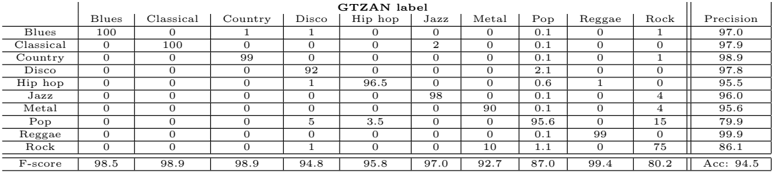This dataset was purposely created to have a variety of fideli- Table 4: The statistics ( × 10 -2 ) of the 'perfect' classifier for GTZAN considering the 59 mislabelings in Table 2, and that the 81 excerpts we have yet to identify have 'correct' labels <details> <summary>Image 3 Details</summary>  ### Visual Description ## Confusion Matrix: GTZAN Label Classification Performance ### Overview The image presents a confusion matrix comparing predicted music genre classifications (rows) against ground truth labels (columns) for the GTZAN dataset. The matrix includes precision metrics for each genre and an overall accuracy score of 94.5%. The data reveals classification performance across 11 music genres with notable variations in precision scores. ### Components/Axes - **Rows**: Predicted genre classifications (Blues, Classical, Country, Disco, Hip hop, Jazz, Metal, Pop, Reggae, Rock) - **Columns**: Ground truth genre labels (Blues, Classical, Country, Disco, Hip hop, Jazz, Metal, Pop, Reggae, Rock) - **Final Column**: Precision scores for each predicted genre - **Bottom Row**: F-scores for each genre (average of precision and recall) - **Accuracy**: 94.5% (bottom-right corner) ### Detailed Analysis 1. **Class-Specific Performance**: - **Blues**: Perfect self-classification (100) with minor errors (1 in Country, 1 in Disco, 1 in Rock). Precision: 97.0% - **Classical**: Dominant self-classification (100) with 2 errors in Jazz. Precision: 97.9% - **Country**: Strong self-classification (99) with 1 error in Rock. Precision: 98.9% - **Disco**: High self-classification (92) with 2 errors in Pop. Precision: 97.8% - **Hip hop**: Dominant self-classification (96.5) with 1 error in Reggae. Precision: 95.5% - **Jazz**: Strong self-classification (98) with 4 errors in Rock. Precision: 96.0% - **Metal**: High self-classification (90) with 4 errors in Rock. Precision: 95.6% - **Pop**: Poor self-classification (5) with 15 errors in Rock. Precision: 79.9% - **Reggae**: Perfect self-classification (99) with 1 error in Hip hop. Precision: 99.9% - **Rock**: Severe misclassification (75 errors) across all genres. Precision: 86.1% 2. **F-Score Trends**: - Highest F-score: Reggae (99.4) - Lowest F-score: Pop (87.0) - Rock shows significant underperformance (80.2 F-score) 3. **Accuracy Context**: - Overall accuracy of 94.5% suggests strong general performance - Discrepancy between high accuracy and low Rock precision indicates class imbalance ### Key Observations 1. **Pop Genre Anomaly**: - Only 5 correct classifications out of 24 total predictions (21% accuracy) - 15 misclassifications as Rock (62.5% of errors) - Lowest precision (79.9%) and F-score (87.0) 2. **Rock Genre Challenges**: - 75 total misclassifications (31.3% of all errors) - High error rates from all other genres (4-15 instances each) - Lowest precision (86.1%) despite being the most frequent misclassification target 3. **Class Imbalance**: - Rock appears to be the most frequent genre in the dataset (75 instances) - Other genres show better self-classification despite lower absolute counts ### Interpretation This confusion matrix reveals a machine learning model trained on the GTZAN dataset with strong overall performance (94.5% accuracy) but significant challenges with specific genres. The Pop genre demonstrates particularly poor classification (79.9% precision), likely due to overlapping characteristics with Rock. The Rock genre's high error rate (75 misclassifications) suggests either: 1. Dataset imbalance favoring Rock samples 2. Model bias toward Rock classification 3. Inherent acoustic similarities between Rock and other genres The high F-scores for Reggae (99.4) and Blues (98.5) indicate these genres have distinct acoustic signatures that the model effectively distinguishes. The Jazz genre's 4 Rock misclassifications (4.1% of total errors) suggest potential confusion between complex rhythmic patterns in these genres. The data implies opportunities for model improvement through: - Balanced dataset curation - Feature engineering emphasizing genre-specific acoustic markers - Ensemble methods to reduce Rock/Pop classification errors </details> | | GTZAN label | GTZAN label | GTZAN label | GTZAN label | GTZAN label | GTZAN label | GTZAN label | GTZAN label | GTZAN label | GTZAN label | GTZAN label | |-----------|---------------|---------------|---------------|---------------|---------------|---------------|---------------|---------------|---------------|---------------|---------------| | | Blues | Classical | Country | Disco | Hip hop | Jazz | Metal | Pop | Reggae | Rock | Precision | | Blues | 100 | 0 | 1 | 1 | 0 | 0 | 0 | 0.1 | 0 | 1 | 97.0 | | Classical | 0 | 100 | 0 | 0 | 0 | 2 | 0 | 0.1 | 0 | 0 | 97.9 | | Country | 0 | 0 | 99 | 0 | 0 | 0 | 0 | 0.1 | 0 | 1 | 98.9 | | Disco | 0 | 0 | 0 | 92 | 0 | 0 | 0 | 2.1 | 0 | 0 | 97.8 | | Hip hop | 0 | 0 | 0 | 1 | 96.5 | 0 | 0 | 0.6 | 1 | 0 | 95.5 | | Jazz | 0 | 0 | 0 | 0 | 0 | 98 | 0 | 0.1 | 0 | 4 | 96.0 | | Metal | 0 | 0 | 0 | 0 | 0 | 0 | 90 | 0.1 | 0 | 4 | 95.6 | | Pop | 0 | 0 | 0 | 5 | 3.5 | 0 | 0 | 95.6 | 0 | 15 | 79.9 | | Reggae | 0 | 0 | 0 | 0 | 0 | 0 | 0 | 0.1 | 99 | 0 | 99.9 | | Rock | 0 | 0 | 0 | 1 | 0 | 0 | 10 | 1.1 | 0 | 75 | 86.1 | | F-score | 98.5 | 98.9 | 98.9 | 94.8 | 95.8 | 97.0 | 92.7 | 87.0 | 99.4 | 80.2 | Acc: 94.5 | ties in the excerpts [92]; however, one of the excerpts (Reggae 86) is so severely distorted that its last 25 seconds are useless. ## 2.6 Estimating statistics of 'perfect' performance We now estimate several figures of merit for the 'perfect' MGR system evaluated using Classify [1] in GTZAN . Table 4 estimates the 'ideal' confusion table, which we construct using the scores of the mislabeled excerpts in Table 2. For instance, Country 39 has its highest score in Blues, so we add one to the Blues label in the Country column. On the other hand, Hip hop 40 has its highest score in Hip hop, but its score in Pop is high enough to consider it significant (per the definition above), so we add 0.5 to both Hip hop and Pop. For Pop 81, where hardly any of the tags match the top tags of the GTZAN labels, we assign a weight of 0.1 to all labels. We also assume that the first 5 seconds of Reggae 86 are representative enough of GTZAN Reggae. Finally, we assume that the 81 excerpts we have yet to identify have 'correct' labels. From Table 4, we can estimate the best recalls (the diagonal), the best precisions (last column), and the best F-scores (last row). The best classification accuracy (bottom right corner) is around 94.5%. Hence, if the classification accuracy of an MGR system tested in GTZAN is better that this, then it might actually be performing worse than the 'perfect' system. ## 3 GTZAN in MGR Research Figure 3 shows how the number of publications that use GTZAN has increased since its creation in 2002. The next most used publicly-available dataset is that created for the ISMIR 2004 MGR contest [117], which appears in 75 works, 30 of which use GTZAN as well [4, 20, 30, 31, 37-39, 47-50, 54, 55, 57, 58, 60-64, 67, 72, 73,75-77,86,94,98,100]. Of the 100 works that use GTZAN , 49 of them only use GTZAN [2, 3, 5, 7-11, 13, 14, 16-19, 21-25, 27, 29, 32-34, 36, 41, 42, 45, 46, 51, 53, 59, 65,66,69,71,74,79-85,91,95-97,101]. Figure 3: Annual numbers of published works in MGR with experimental components, divided into ones that use and do no use GTZAN . <details> <summary>Image 4 Details</summary>  ### Visual Description ## Bar Chart: Publications Using vs. Not Using GTZAN (2002–2012) ### Overview The chart compares annual publications categorized by whether they used the GTZAN tool (black bars) or did not use it (gray bars) from 2002 to 2012. The y-axis represents the number of publications, ranging from 0 to 70. The x-axis spans 11 years, with data points for each year. ### Components/Axes - **X-axis (Years)**: 2002, 2003, 2004, 2005, 2006, 2007, 2008, 2009, 2010, 2011, 2012. - **Y-axis (Publications)**: Scale from 0 to 70, with increments of 10. - **Legend**: Located in the top-left corner. Black bars = "using GTZAN"; Gray bars = "not using GTZAN". - **Bars**: Each year has two stacked bars (black for "using," gray for "not using"). ### Detailed Analysis - **2002**: 2 (using GTZAN), 11 (not using GTZAN). - **2003**: 2 (using GTZAN), 18 (not using GTZAN). - **2004**: 1 (using GTZAN), 27 (not using GTZAN). - **2005**: 5 (using GTZAN), 32 (not using GTZAN). - **2006**: 8 (using GTZAN), 41 (not using GTZAN). - **2007**: 3 (using GTZAN), 30 (not using GTZAN). - **2008**: 6 (using GTZAN), 38 (not using GTZAN). - **2009**: 9 (using GTZAN), 49 (not using GTZAN). - **2010**: 22 (using GTZAN), 65 (not using GTZAN). - **2011**: 19 (using GTZAN), 55 (not using GTZAN). - **2012**: 20 (using GTZAN), 47 (not using GTZAN). ### Key Observations 1. **Rising Trend for "Not Using GTZAN"**: Publications not using GTZAN consistently increase from 11 (2002) to 65 (2010), peaking in 2010 before declining to 47 (2012). 2. **Peak for "Using GTZAN" in 2010**: The highest number of publications using GTZAN (22) occurs in 2010, followed by a sharp decline to 20 (2012). 3. **Widening Gap (2002–2010)**: The difference between "not using" and "using" GTZAN grows from 9 (2002) to 43 (2010). 4. **Narrowing Gap (2010–2012)**: After 2010, the gap reduces from 43 to 27 (2012), suggesting increased adoption of GTZAN post-2010. ### Interpretation - **Adoption Surge (2010)**: The peak in GTZAN usage in 2010 may reflect a methodological shift, tool optimization, or increased awareness. However, the subsequent decline suggests potential saturation, competition from alternative tools, or a return to prior practices. - **Dominance of "Not Using"**: Until 2010, publications not using GTZAN far outnumbered those using it, indicating limited adoption. Post-2010, the gap narrows, but "not using" remains dominant. - **Anomalies**: The drop in "using GTZAN" after 2010 (22 → 20) and the decline in "not using" (65 → 47) could signal a stabilization or cyclical trend. The 2007 dip in "not using" (30) might indicate a temporary spike in GTZAN adoption that year. The data highlights a critical inflection point in 2010, where GTZAN usage reached its zenith, followed by a reversal. This could reflect evolving academic or industry standards, tool limitations, or external factors influencing publication practices. </details> ## 3.1 Listening to GTZAN Among 100 works, we find only five (outside our recent work [83-86]), that indicate someone has listened to at least some of GTZAN . The first appears to be Li and Sleep [42], who find that '... two closely numbered files in each genre tend to sound similar than the files numbered far [apart].' Bergstra et al. [12] note that, 'To our ears, the examples are well-labeled ... our impression from listening to the music is that no artist appears twice.' This is contradicted by Seyerlehner et al. [76], who predict 'an artist effect ... as listening to some of the songs reveals that some artists are represented with several songs.' In his doctoral dissertation, Seyerlehner [75] infers there to be a significant replication of artists in GTZAN because of how classifiers trained and tested in that dataset perform as compared to other artist-filtered datasets. Very few works mention specific faults in GTZAN . Hartmann [28] notes finding seven duplicates, but mentions no specifics. In [15,56,71,74], the authors describe GTZAN as having 993 or 999 excerpts. In personal communication, de los Santos mentions that they found seven corrupted files in Classical (though [71,74] report them being in Reggae). Li and Chan [46], who manually estimate the key of all GTZAN excerpts, mention in personal communication that they remember hearing some repetitions. Their key estimates 4 are consistent among the exact repetitions we find in GTZAN . ## 3.2 Using GTZAN In our review of evaluation in MGR [1], we delimit ten different experimental designs. In the 100 works using GTZAN , 96 employ the experimental design Classify [2-14,16-18,20-76,78-100] (an excerpt is assigned a class, and that class is compared against a 'ground truth'). In seven papers, GTZAN is used with the design Retrieve [15,19,22,38,77,79,101] (a query is used to find similar music, and the labels of the retrieved items are compared). The work in [8] uses GTZAN in 4 http://visal.cs.cityu.edu.hk/downloads/#gtzankeys the design Cluster (data is clustered, and the composition of the resulting clusters are inspected). Our work in [83] uses Compose , where a system is trained on GTZAN , and then generates music it finds highly representative of each GTZAN label. With a formal listening test of these representative excerpts, we find humans cannot recognize the genres they supposedly represent. 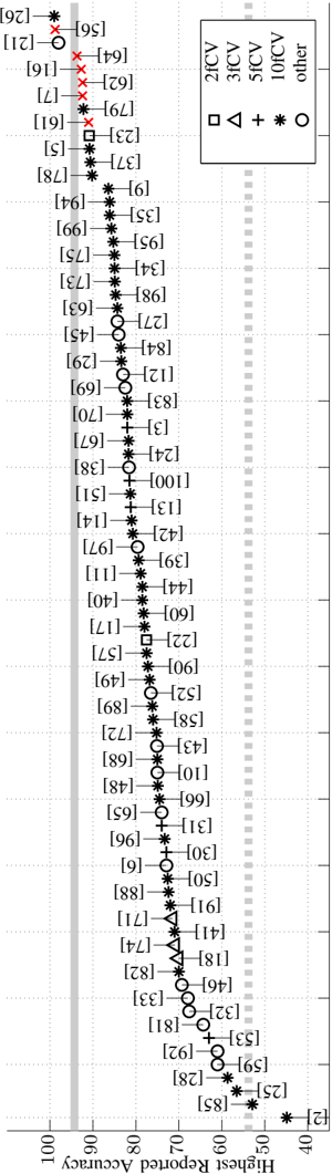The design parameters in these works vary. For Classify , most works measure MGR performance by classification accuracy (the ratio of 'correct' predictions to all observations) computed from k -fold stratified cross-validation ( k fCV), e.g., 2fCV (4 papers) [7,22,23,56], 3fCV (3 papers) [18,71,74], 5fCV (6 papers) [3,13,30, 31,53,100], and 10fCV (55 papers) [2,5,9,11,14,16,17,24-26,28,29,34,35,37,39-42, 44,47-51,57,58,60-64,66-68,70,72,73,75,76,78,79,82-85,88-91,94-96,98,99]. Most of these use a single run of cross-validation; however, some perform multiple runs, e.g., 10 independent runs of 2fCV (10x2CV) [56] or 20x2fCV [22, 23], 10x3fCV [71,74], and 10x10fCV [37,70,72,75,83-85]. In one experiment, Li and Sleep [42] use 10fCV with random partitions; but in another, they partition the excerpts into folds based on their file number - roughly implementing an artist filter. Finally, leave one out cross-validation appears in [32,33]. Some works measure classification accuracy using a split of the data, e.g., 60/40 [8] (60% used to train, 40% used to test), 70/30 [10,43], 75/25 [59], 80/20 [12,45,52,65], 90/10 [10,81,92,93,97], and training/validation/testing of 50/20/30 [27]. Half of these report results from a single split [8, 10, 12, 27, 45, 52]; but the other half reports a mean of many trials, e.g., 5 [43], 30 [97], and 100 trials [65, 81, 92, 93]. Seven papers [6, 21, 38, 56, 59, 69, 87] do not coherently describe their design parameters. In some cases, only a portion of GTZAN is used, e.g., [4] performs 5x5fCV using only Classical, Jazz and Pop; [36] uses Blues, Classical, Country and Disco; [80] uses several combinations of GTZAN categories; and [20] states a three-genre subset is used, but provide no details on which they use. Other works add to GTZAN , e.g., [8] adds 100 excerpts of Portuguese music to GTZAN Classical, Metal, and Reggae; [87] augments the excerpts in Classical and Jazz with recordings of internet radio; and [46] uses all of GTZAN , and augments it with pitch-shifted and/or time-scaled versions. Figure 4: Highest classification accuracies (y-axis) reported (cross-references labeled) with experimental design Classify using all GTZAN . Shapes (legend) denote particular details of the experimental procedure, e.g., '2fCV' is two-fold cross validation; 'other' means randomly partitioning data into training/validation/test sets, or an unspecified experimental procedure. Five 'x' denote results that have been challenged, and/or shown to be invalid. Solid gray line is our estimate of the 'perfect' accuracy in Table 2. Dashed gray line is the best accuracy of the five systems in Section 4 that we evaluate using fault <details> <summary>Image 5 Details</summary>  ### Visual Description ## Line Chart: Accuracy vs. Highest Reported Accuracy ### Overview The image is a line chart comparing the "Highest Reported Accuracy" (x-axis) against "Accuracy" (y-axis). Multiple data series are represented by distinct symbols and colors, with a legend in the top-right corner. The chart includes a vertical line at x=90 and a dashed horizontal line at y=50. Data points are plotted along the y-axis, with numerical labels in brackets. ### Components/Axes - **X-axis (Highest Reported Accuracy)**: Ranges from 100 (left) to 40 (right), with a vertical line at 90. - **Y-axis (Accuracy)**: Discrete numerical values (e.g., 26, 56, 21, etc.) labeled in brackets. - **Legend**: Located in the top-right corner, with the following mappings: - **2fcV**: Square (□) - **3fcV**: Triangle (△) - **5fcV**: Plus (+) - **10fcV**: Asterisk (*) - **Other**: Circle (○) ### Detailed Analysis - **Data Series Trends**: - **10fcV (asterisks)**: Highest accuracy values, clustered near the top of the y-axis (e.g., 100, 99, 95). - **5fcV (pluses)**: Slightly lower than 10fcV, with values like 97, 94, 93. - **3fcV (triangles)**: Lower than 5fcV, with values such as 92, 89, 88. - **2fcV (squares)**: Lower still, with values like 85, 83, 81. - **Other (circles)**: Lowest accuracy, with values like 79, 77, 75. - **Key Data Points**: - Highest reported accuracy: **100** (y=100, x=100). - Lowest reported accuracy: **40** (y=40, x=40). - Vertical line at x=90 separates higher (left) and lower (right) accuracy ranges. - Dashed horizontal line at y=50 may indicate a threshold for acceptable accuracy. ### Key Observations - **Clustering**: Data points are densely packed between y=50 and y=100, with fewer points below y=50. - **Outliers**: A few data points (e.g., y=26, y=21) fall below y=50, suggesting lower accuracy for specific cases. - **Legend Consistency**: Symbols match their corresponding data series (e.g., asterisks for 10fcV). ### Interpretation The chart demonstrates a clear trend where higher fcV values (e.g., 10fcV) correlate with higher reported accuracy. The vertical line at x=90 may represent a benchmark or target for accuracy, while the dashed line at y=50 could signify a minimum acceptable threshold. The "other" category (circles) consistently shows lower accuracy compared to the fcV series, indicating potential differences in performance or methodology. The data suggests that increasing fcV values improves accuracy, though exceptions exist (e.g., lower accuracy for some 2fcV or 3fcV cases). This could imply that fcV is a critical factor in determining accuracy, but further analysis is needed to confirm causality. </details> filtering. In summary, we find that about half of the work using GTZAN uses no other dataset, which means that a majority of evaluations can provide no conclusions about the performance of a system on other datasets, e.g., in the real world [104, 105]. Since 96 of 100 papers use Classify to evaluate MGR systems, most papers report classification accuracy as a figure of merit, and some work use this figure to compare systems for recognizing music genre. We have criticized this approach to evaluation [84], and argued that it lacks the validity necessary to make any meaningful comparisons between systems [105]. ## 3.3 Reported classification accuracies in GTZAN Figure 4 shows the highest classification accuracies reported in 96 papers that consider the 10-class problem of GTZAN (we remove duplicated experiments, e.g., [48] contains the results reported in [47]). The thick gray line in Fig. 4 shows our estimate of the 'perfect' classification accuracy from Table 4. Six results (marked with a red 'x') are incorrect or have been challenged: the results in [61,62,64] are due to a mistake in the experimental procedure [84], as are those in [56]; 5 the result in [16] contradicts many others [85]; and the results in [7] are not likely to come from the system [118]. ## 4 The faults of GTZAN and evaluation In this section, we disprove the following two claims: 1) 'all MGR systems and evaluations are affected in the same ways by the faults in GTZAN '; and 2) 'the performances of all MGR systems in GTZAN , working with the same data and faults, are still meaningfully comparable.' Such claims have been made in reviews of this work, but also appear in [99]. We now study how the faults of GTZAN affect the evaluation of MGR systems, e.g., the estimation of classification accuracy using Classify in GTZAN . It is not difficult to predict how these faults can affect the evaluations of particular systems. For instance, when exact replicas are distributed across train and test sets, the evaluation of some systems can be more biased than others: a nearest neighbor classifier will find features in the training set with zero distance to the test feature, while a Bayesian classifier with a parametric model may not so strongly benefit when its model parameters are estimated from all training features. If there are replicas in the test set only, then they will bias our estimate of a figure of merit because they are not independent tests - if one is classified (in)correctly then its replicas are also classified (in)correctly. Thus, we already have a notion that the two claims above are not true. In addition to exact repetitions, we show above that the number of artists in GTZAN is at most 329. Thus, as Seyerlehner [75, 76] predicts for GTZAN , the evaluation of systems will certainly be biased due to the artist effect [119-122], i.e., the observation that a music similarity system can perform significantly worse 5 Personal communication with J. P. Papa. when artists are disjoint in training and test datasets, than when they are not. Since all results in Fig. 4 come from evaluations without an artist filter, they will likely be optimistic. What has yet to be shown for GTZAN , however, is just how optimistic they might be. After presenting our experimental method, we then present our results, and discuss the veracity of the two claims above. ## 4.1 Method We use three classifiers with the same features [123]: nearest neighbor (NN); minimum distance (MD); and minimum Mahalanobis distance (MMD). We implement these classifiers in PRTools [124]. We create feature vectors from a 30-s excerpt in the following way. For each 46.4 ms frame, and a hop half that, we compute: 13 MFCCs using the approach in [125], zero crossings, and spectral centroid and rolloff. For each 130 consecutive frames, we compute the mean and variance of each dimension, thus producing nine 32-dimensional feature vectors for each excerpt. We normalize the dimensions of the training set features, i.e., we find and apply the transformation mapping each dimension to [0 , 1]. We apply the same transformation to the test set. Each classifier labels an excerpt as follows: NN randomly selects among the majority labels given to the nine feature vectors; MD and MMD both select the label with the maximum log posterior sum over the nine feature vectors. In addition to there, we test two state-of-the-art MGR systems that produce some of the highest classification accuracies reported in GTZAN . The first is SRCAM - proposed in [61] and modified in [84] - which uses psychoacousticallymotivated features in 768 dimensions. SRCAM classifies an excerpt by sparse representation classification [126]. We use the SPGL1 solver [127] with at most 200 iterations, and 2 := 0 . 01. The second system is MAPsCAT, which uses features computed with the scattering transform [3]. This produces 40 feature vectors of 469 dimensions for a 30-s excerpt. MAPsCAT estimates from the training set the mean for each class, the total covariance matrix, and computes for a test feature the log posterior in each class. We define all classes equally likely for MAPsCAT, as well as MD and MMD. We normalize the features of the training and test sets. We give further details of SRCAM and MAPsCAT in [84]. 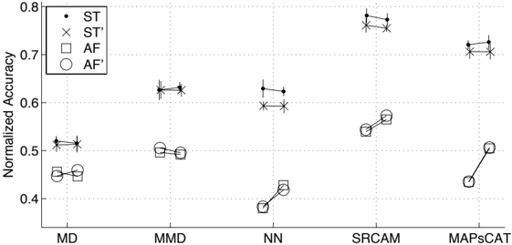We evaluate each system using GTZAN with four different kinds of partitioning: ten realizations of standard non-stratified 2fCV (ST); ST without the 68 exact and recording repetitions and 2 distortions (ST'); a non-stratified 2fCV with artist filtering (AF); AF without the 68 exact and recording repetitions and 2 distortions (AF'). Table 5 shows the composition of each fold of AF in terms of artists. We created AF manually to ensure that: 1) each class is approximately balanced in terms of the number of training and testing excerpts; and 2) each fold of a class has music representative of its top tags (Fig. 2). For instance, the Blues folds have 46 and 54 excerpts, and both have Delta blues and zydeco. We retain the original labels of all excerpts, and evaluate all systems using the same partitions. We look at several figures of merit: confusion, precision, recall, F-score, and Table 5: Composition of each fold of the artist filter partitioning (500 excerpts in each). Italicized artists appear in two categories. | | Fold 1 | Fold 2 | |-----------|------------------------------------------------------------------------------------------------------------------------|--------------------------------------------------------------------------------------------------------| | Blues | John Lee Hooker, Kelly Joe Phelps, Buck- wheat Zydeco, Magic Slim & The Teardrops | Robert Johnson, Stevie Ray Vaughan, Clifton Chenier, Hot Toddy, Albert Collins | | Classical | J. S. Bach, Percy Grainger, Maurice Ravel, Henri Dutilleux, Tchaikovsky, Franz Schu- bert, Leonard Bernstein , misc. | Beethoven, Franz Joseph Haydn, Mozart, Vi- valdi, Claude Debussy, misc. | | Country | Shania Twain, Johnny Cash, Willie Nelson, misc. | Brad Paisley, George Strait, Vince Gill, misc. | | Disco | Donna Summer, KC and The Sunshine Band, Ottawan, The Gibson Brothers, Heatwave, Evelyn Thomas, misc. | Carl Douglas, Village People, The Trammps, Earth Wind and Fire, Boney M., ABBA, Glo- ria Gaynor, misc. | | Hip hop | De La Soul, Ice Cube, Wu-Tang Clan, Cypress Hill, Beastie Boys, 50 Cent, Eminem, misc. | A Tribe Called Quest, Public Enemy, Lauryn Hill , Wyclef Jean | | Jazz | Leonard Bernstein , Coleman Hawkins, Bran- ford Marsalis Trio, misc. | James Carter, Joe Lovano, Dexter Gordon, Tony Williams, Miles Davis, Joe Henderson, misc. | | Metal | Judas Priest, Black Sabbath, Queen , Dio, Def Leppard, Rage Against the Machine, Guns N' Roses , New Bomb Turks, misc. | AC/DC, Dark Tranquillity, Iron Maiden, Ozzy Osbourne, Metallica, misc. | | Pop | Mariah Carey, Celine Dion, Britney Spears, Alanis Morissette, Christina Aguilera, misc. | Destiny's Child, Mandy Moore, Jennifer Lopez, Janet Jackson, Madonna, misc. | | Reggae | Burning Spear, Desmond Dekker, Jimmy Cliff, Bounty Killer, Dennis Brown, Gregory Isaacs, Ini Kamoze, misc. | Peter Tosh, Prince Buster, Bob Marley, Lau- ryn Hill , misc. | | Rock | Sting, Simply Red, Queen , Survivor, Guns N' Roses , The Stone Roses, misc. | The Rolling Stones, Ani DiFranco, Led Zep- pelin, Simple Minds, Morphine, misc. | classification accuracy. Consider that the i th fold of a cross-validation experiment consists of N ( g ) i excerpts of label g ∈ G , and that of these a system classifies as r ∈ G the number M ( g as r ) i ≤ N (g) i . We define the confusion of label g as r of this fold as $$C _ { i } ^ { ( g as r ) } = M _ { q } ^ { ( g as r ) } / N _ { i } ^ { ( g as r ) }$$ Thus, C ( g as g ) i is the recall for class g in the i th fold. The normalized accuracy of a system in the i th fold is defined by $$A _ { 1 } = \frac { 1 } { \vert G \vert } \sum C _ { i } ^ { ( g as g ) }$$ We use normalized accuracy because the classes are not equally represented in the test sets. Finally, the precision of a system for class X in the i th fold is and the F-score of an system for label X in the i th fold is $$F _ { i } ^ { ( X ) } \cdot = 2 P ( X _ { i } C ( X as X ) / | P ( X _ { i } )$$ To test for significant differences in performance between two systems, we first build contingency tables for all observations they classify [128]. Define the rv N to Figure 5: Normalized accuracy (7) of each system (x-axis) for each fold (left and right) of different partitioning (legend). <details> <summary>Image 6 Details</summary>  ### Visual Description ## Scatter Plot: Normalized Accuracy Across Model Categories ### Overview The image is a scatter plot comparing normalized accuracy values across five model categories (MD, MMD, NN, SRCAM, MAPsCAT) for four distinct data series (ST, ST', AF, AF'). The plot uses distinct symbols and colors to differentiate the series, with error bars indicating variability. ### Components/Axes - **X-Axis (Categories)**: Labeled with model types: MD, MMD, NN, SRCAM, MAPsCAT. - **Y-Axis (Normalized Accuracy)**: Scaled from 0.4 to 0.8 in increments of 0.1. - **Legend**: Located in the top-left corner, mapping symbols to series: - **ST**: Filled black circles (●) - **ST'**: Black crosses (✖) - **AF**: Open black squares (■) - **AF'**: Open black circles (○) - **Error Bars**: Present for all data points, suggesting measurement uncertainty. ### Detailed Analysis 1. **MD Category**: - **ST**: ~0.52 (●) - **ST'**: ~0.51 (✖) - **AF**: ~0.47 (■) - **AF'**: ~0.46 (○) 2. **MMD Category**: - **ST**: ~0.63 (●) - **ST'**: ~0.62 (✖) - **AF**: ~0.50 (■) - **AF'**: ~0.50 (○) 3. **NN Category**: - **ST**: ~0.61 (●) - **ST'**: ~0.59 (✖) - **AF**: ~0.38 (■) - **AF'**: ~0.42 (○) 4. **SRCAM Category**: - **ST**: ~0.76 (●) - **ST'**: ~0.75 (✖) - **AF**: ~0.55 (■) - **AF'**: ~0.54 (○) 5. **MAPsCAT Category**: - **ST**: ~0.72 (●) - **ST'**: ~0.71 (✖) - **AF**: ~0.48 (■) - **AF'**: ~0.50 (○) ### Key Observations - **ST and ST' Consistently Outperform AF and AF'**: Across all categories, ST and ST' achieve higher normalized accuracy than AF and AF'. - **SRCAM Dominates**: SRCAM shows the highest accuracy for both ST (~0.76) and ST' (~0.75), suggesting it is the most effective model for these series. - **MAPsCAT Weakness**: MAPsCAT has the lowest accuracy for AF (~0.48) and AF' (~0.50), indicating potential limitations in handling these series. - **NN Anomaly**: NN exhibits a significant drop in AF accuracy (~0.38), the lowest observed value for any series. ### Interpretation The data suggests that ST and ST' (likely supervised or semi-supervised methods) outperform AF and AF' (possibly unsupervised or feature-based approaches) across most model categories. SRCAM’s superior performance for ST/ST' implies it may leverage structural or relational patterns effectively. The NN’s poor AF performance could indicate overfitting or insufficient feature extraction for unsupervised tasks. MAPsCAT’s middling results for AF/AF' suggest moderate adaptability but limited robustness compared to SRCAM. Error bars highlight variability, emphasizing the need for larger datasets or refined models to reduce uncertainty. </details> be the number of times the two systems choose different classes, but one is correct. Let t 12 be the number for which system 1 is correct but system 2 is wrong. Thus, N -t 12 is the number of observations for which system 2 is correct but system 1 is wrong. Define the rv T 12 from which t 12 is a sample. The null hypothesis is that the systems perform equally well given N = n , i.e., E [ T 12 | N = n ] = n/ 2, in which case T 12 is distributed binomial, i.e., $$t \leq n . ( 1 0 )$$ The probability we observe a particular performance given the systems perform equally well is $$\sum _ { t = 0 } ^ { n - t _ { 1 2 } } P [ T _ { 1 2 } \leq t _ { 1 2 } , n - t _ { 1 2 } ] + P [ T _ { 1 2 } \geq t _ { 1 2 } , n - t _ { 1 2 } ]$$ We define statistical significance as α = 0 . 05. In other words, we reject the null hypothesis when p < α . ## 4.2 Experimental results and discussion Figure 5 shows the normalized accuracies (7) of all five systems for each fold of the four different kinds of partitioning. For the ten partitions of ST and ST', we show the mean normalized accuracy, and one standard deviation above and below. It is immediately clear that estimates of the classification accuracy for each system are affected by the faults of GTZAN . We see that the differences between ST and ST' are small for all systems except NN. As we predict above, the performance of NN appears to benefit more than the others from the exact and recording repetitions, which boost its mean normalized accuracy from about 0.6 to 0.63. Between AF and AF', removing the repetitions produces very little change since the artist filter keeps exact and recording repetitions from appearing in both train and test sets. Most clearly, we see for all five systems large decreases in performance between ST and AF. The difference in normalized accuracy of MD between ST and AF appears the smallest (7 points), while that of MAPsCAT appears the most (25 points). Since we have thus found systems with performance evaluations affected to different magnitudes by the faults in GTZAN -that of NN is hurt by removing the repetitions while that of MMD is not - this disproves the first claim above. Testing for significant difference in performance between all pairs of system in both ST and ST', only for MMD and NN do we fail to reject the null hypothesis. Furthermore, in terms of classification accuracy in ST, we can say with statistical significance: MD < { MMD, NN } < MAPsCAT < SRCAM, i.e., SRCAM performs the best and MD performs the worst. In both AF and AF', however, for MAPsCAT and MD, and for MAPsCAT and MMD, do we fail to reject the null hypothesis. In this case, we can say with statistical significance: NN < { MAPsCAT, MD } < { MAPsCAT, MMD } < SRCAM. Therefore, while our conclusion on the basis of our evaluation in ST is that MAPsCAT performs significantly better than all these systems except SRCAM, its evaluation in AF says otherwise. This disproves the second claim above. 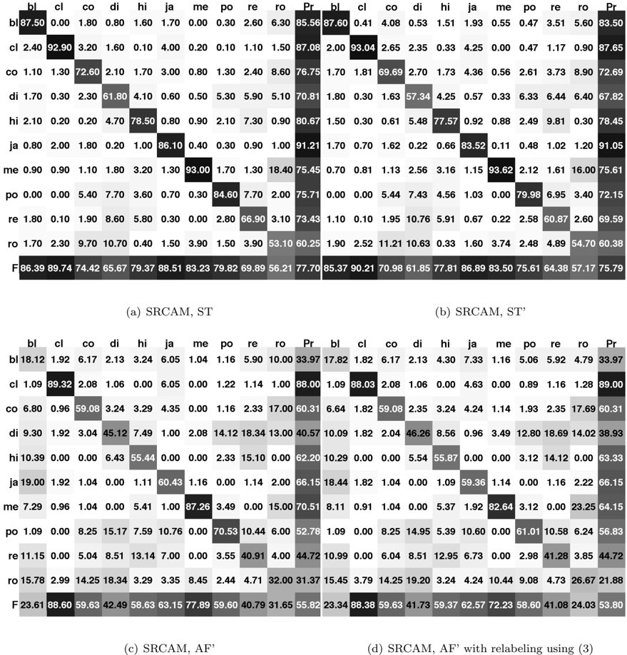We now focus our analysis upon SRCAM. Figure 6 shows other figures of merit for SRCAM averaged over 10 realizations of ST and ST' partitions, as well as for the single partition AF'. Between ST and ST', we see very little change in the recalls for classes with the few exact and recording repetitions: Blues, Classical and Rock. However, for the classes having the most exact and recording repetitions, we find large changes in their recalls. In fact, Fig. 7 shows that the number of exact and recording repetitions in a category is correlated with a decrease in its recall for SRCAM. This makes sense as SRCAM can be seen as a kind of adaptive nearest neighbors. When evaluating SRCAM in AF', Fig. 6 shows our estimate of its classification accuracy in ST decreases by 22 points (28%). With respect to F-score, Classical appears to suffers the least; but we see decreases for all other classes by at least 10%, e.g., 77% for Blues, 46% for Rock, and 44% for Reggae. We see little change in our estimated classification accuracy when testing in AF' instead of AF (not shown), but our estimates of recalls, precisions, and F-scores for four classes increase, while those for thee classes decrease. In all figures of merit above, we have not considered the 59 mislabelings in GTZAN noted in Table 2. We thus assign new labels to each of the 59 excerpts based on which class has highest score (3) for the excerpt. If the score is zero in every class, e.g., Pop 81, we keep the original label. We assume that the 81 excerpts we have yet to identify have 'correct' labels. The new figures of merit for SRCAM, seen in Fig. 6(d), show even further deterioration. Compared to the figures of merit in ST, we are quite far from the 'perfect' statistics in Table 4. Figure 6: Confusion, precision (Pr), F-score (F), and normalized accuracy (bottom right corner) for SRCAM evaluated with (ST) and without repetitions (ST') averaged over 10 realizations, as well as with artist filtering and without replicas (AF'), and finally taking mislabelings into account. Columns are 'true' labels; rows are predictions. Darkness of square corresponds to value. Labels: Blues (bl), Classical (cl), Country (co), Disco (di), Hip hop (hi), Jazz (ja), Metal (me), Pop (po), Reggae (re), Rock (ro). <details> <summary>Image 7 Details</summary>  ### Visual Description ## Heatmaps: SRCAM Model Performance Comparison ### Overview The image contains four comparative heatmaps (a-d) visualizing performance metrics across different configurations of the SRCAM model. Each heatmap uses a color gradient (light to dark) to represent numerical values, with darker shades indicating higher values. The matrices compare pairwise relationships between 11 categories (bl, cl, co, di, hi, ja, me, po, re, ro, Pr) across four experimental setups. ### Components/Axes - **Rows & Columns**: 11 categories labeled with abbreviations: - bl, cl, co, di, hi, ja, me, po, re, ro, Pr - **Legend**: Implied color scale (light = low values, dark = high values) - **X-axis**: Column categories (same as rows) - **Y-axis**: Row categories (same as columns) - **Annotations**: Numerical values in each cell - **Subtitles**: - (a) SRCAM, ST - (b) SRCAM, ST' - (c) SRCAM, AF' - (d) SRCAM, AF' with relabeling using (3) ### Detailed Analysis #### (a) SRCAM, ST - **Highest Value**: 93.00 (ja row, me column) - **Lowest Value**: 0.00 (multiple cells) - **Notable Pattern**: Diagonal dominance with high values along the main diagonal (e.g., 86.10 at ja/ja) #### (b) SRCAM, ST' - **Highest Value**: 93.62 (ja row, me column) - **Lowest Value**: 0.00 (multiple cells) - **Notable Pattern**: Similar diagonal structure to (a), but with increased values in off-diagonal cells (e.g., 88.00 at cl/cl) #### (c) SRCAM, AF' - **Highest Value**: 88.60 (F row, cl column) - **Lowest Value**: 0.00 (multiple cells) - **Notable Pattern**: More uniform distribution with high values in F row (average across categories) #### (d) SRCAM, AF' with relabeling using (3) - **Highest Value**: 93.38 (Pr row, Pr column) - **Lowest Value**: 0.00 (multiple cells) - **Notable Pattern**: Significant improvement in diagonal values (e.g., 93.38 at Pr/Pr) and reduced off-diagonal variability ### Key Observations 1. **Relabeling Impact**: Heatmap (d) shows consistent improvements in diagonal values (e.g., Pr/Pr increases from 83.50 in (c) to 93.38 in (d)) 2. **Category Performance**: - 'ja' category consistently shows high values across all configurations - 'Pr' category demonstrates the most dramatic improvement in (d) 3. **F Row Trends**: Average performance (F row) increases slightly from (a) 77.70 to (d) 55.80, suggesting overall model improvement ### Interpretation The heatmaps reveal that the SRCAM model's performance improves significantly when combined with relabeling using (3) (configuration d). The diagonal dominance across all configurations suggests the model maintains strong intra-category relationships. The 'F' row averages indicate that relabeling (d) achieves better overall performance despite some category-specific variations. The consistent high values in 'ja' and 'Pr' categories suggest these are particularly well-represented in the model's output space. The relabeling technique appears to enhance model consistency across categories while maintaining strong diagonal relationships. </details> Figure 7: Scatter plot of percent change in mean figures of merit (FoM) in Fig. 6 between ST and ST' as a function of the number of exact and recording repetitions in a class. 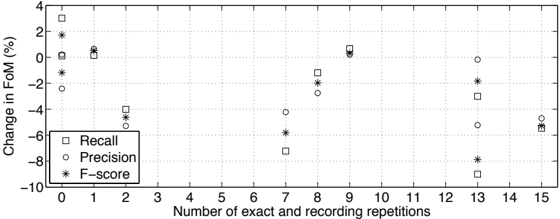<details> <summary>Image 8 Details</summary>  ### Visual Description ## Line Chart: Change in FOM (%) vs. Number of Exact and Recording Repetitions ### Overview The image is a line chart displaying the relationship between the number of exact and recording repetitions (x-axis) and the percentage change in FOM (y-axis). Three data series are represented: Recall (squares), Precision (circles), and F-score (stars). The chart uses a grid background with dotted lines and a legend in the bottom-left corner. ### Components/Axes - **X-axis**: "Number of exact and recording repetitions" (integer values from 0 to 15). - **Y-axis**: "Change in FOM (%)" (ranging from -10% to 4%). - **Legend**: Located in the bottom-left corner, with symbols: - **Recall**: Square (□) - **Precision**: Circle (●) - **F-score**: Star (★) ### Detailed Analysis - **Recall (□)**: - Data points at x = 0, 1, 2, 5, 8, 9, 13, 15. - Values: ~2% (x=0), ~0% (x=1), ~-4% (x=2), ~0% (x=5), ~2% (x=8), ~-2% (x=9), ~-4% (x=13), ~-6% (x=15). - **Precision (●)**: - Data points at x = 0, 1, 2, 5, 7, 8, 9, 13, 15. - Values: ~-2% (x=0), ~0% (x=1), ~-2% (x=2), ~-4% (x=5), ~-2% (x=7), ~0% (x=8), ~-2% (x=9), ~-4% (x=13), ~-6% (x=15). - **F-score (★)**: - Data points at x = 0, 1, 2, 5, 7, 8, 9, 13, 15. - Values: ~2% (x=0), ~-4% (x=1), ~-6% (x=2), ~-4% (x=5), ~-6% (x=7), ~-4% (x=8), ~-6% (x=9), ~-8% (x=13), ~-6% (x=15). ### Key Observations 1. **General Trend**: All three metrics show a **downward trend** as the number of repetitions increases. 2. **Recall**: Peaks at x=8 (~2%) but declines sharply to ~-6% at x=15. 3. **Precision**: Fluctuates but ends at ~-6% at x=15. 4. **F-score**: Consistently negative, reaching ~-8% at x=13 and recovering slightly to ~-6% at x=15. 5. **Outliers**: - Recall and Precision show minor recoveries at x=8 (e.g., ~2% for Recall). - F-score has a sharp drop to ~-8% at x=13. ### Interpretation The data suggests that increasing the number of exact and recording repetitions correlates with a **decline in performance metrics** (Recall, Precision, F-score). This could indicate **overfitting** or **diminishing returns** in the model being evaluated. The F-score, which balances precision and recall, demonstrates the most significant deterioration, implying that the model's overall effectiveness worsens with higher repetition counts. The minor recoveries observed at certain points (e.g., x=8) may reflect temporary improvements due to specific data characteristics or anomalies. The consistent negative trend across all metrics highlights a critical trade-off between repetition frequency and model performance. </details> Table 6: For SRCAM, confusions as Classical, and confusions of Classical. Excerpt numbers in parentheses. | | Non-Classical classified as Classical | Classical misclassifications | |---------|---------------------------------------------------------------------------------------------------------------------------------------------------------------------------------------|----------------------------------------------------------------------------------------------------------------------| | Blues | 'Sugar Mama' John Lee Hooker (5) | 'Ainsi la nuit for String Quartet: VII' Henri Du- tilleux (41); 'Fuge F¨ ur Klavier' Richard Strauss (45) | | Country | 'San Antonio Rose' Floyd Cramer (17); 'My Heroes Have Always Been Cowboys' Willie Nelson (69) | 'Ainsi la nuit for String Quartet: I' Henri Du- tilleux (38) | | Disco | 'WHY?' Bronski Beat (94) | 'Konzert F¨ ur Waldhorn Mit Orchester, Allegro' Richard Strauss (43); 'Violin Concerto No. 1' Karol Szymanowski (46) | | Jazz | ''Round Midnight' James Carter (2); 'You Never Told Me That You Care' James Carter (3); 'My Blue Heaven' Coleman Hawkins (41); 'There Will Never Be Another You' Coleman Hawkins (57) | unidentified (61); 'Piano Sonata No.21 in B flat, D.960, Scherzo' Franz Schubert (65) | | Metal | | 'Solemn Mass for Feast of Santa Maria della Salute' Giovanni Rovetta (56) | | Pop | 'I want you to need me' Celine Dion (40) | | | Reggae | 'Reggae Hit the Town' The Ethiopians (43) | | | Rock | 'The Song Remains The Same' Led Zep- pelin (39) | 'Symphony 6, mvt. 1' Tchaikovsky (51); 'Can- dide Overture' Leonard Bernstein (52) | Based on these results, one might be inclined to argue that, though it is clearly performing poorly overall, SRCAM appears to recognize when music uses the classical genre. This appearance evaporates when we see in Table 6 what Classical excerpts SRCAM confuses for Blues, Country, Disco, Jazz, Metal, and Rock, and which non-Classical excerpts SRCAM confuses for Classical. This argues the contrary that SRCAM has some capacity to recognize when music uses the classical genre. (We see the same kinds of catastrophic failures for Metal, the other class for which SRCAM appears to do well.) ## 5 Conclusions on the future use of GTZAN It should now be incontrovertible that since all 96 systems in Fig. 4 are evaluated using GTZAN in ST, we are unable to judge which is good at reproducing the labels in GTZAN when efforts are taken to deal with the faults of GTZAN , let alone which, if any, has any capacity to recognize genres used by music in the real world, and is thus useful for MGR . MAPsCAT and SRCAM, previously evaluated in GTZAN to have classification accuracies of 83% using ST [83,84], now sit at the bottom of Fig. 4. Where all the others lie, we do not yet know; but we now know that these were two systems with classification accuracies superior to 56 others in Fig. 4. Furthermore, the picture becomes more bleak when we scratch below the surface: for the class in which its figures of merit are the best, SRCAM shows behaviors that are utterly confusing if it really is recognizing that genre. One might now hold little hope that GTZAN has ever been or could ever be useful for tasks such as evaluating systems for MGR, audio similarity, autotagging, etc. However, we have done just that in our analysis above, as well as in previous work [83, 84]. A proper analysis of the results of an MGR system tested on GTZAN must take care of the content of GTZAN , i.e., the music. It is not a question of what figure of merit to use, but of how to draw a valid conclusion with an experimental design that determines whether the decisions and behaviors of a system are related to the musical content that is supposedly behind those decisions [105]. Some argue that our litany of faults above ignores what they say is the most serious problem with GTZAN : that it is too small to produce meaningful results. In some respects, this is justified. While personal music collections may number thousands of pieces of music, commercial datasets and library archives number in the millions. The 1000 excerpts of GTZAN can certainly be argued an insufficient random sample of the population of excerpts 'exemplary' of the genres between which one wishes a useful MGR system to discriminate. Hence, one might argue, it is unreasonably optimistic to assume an MGR system can learn from a fraction of GTZAN those characteristics common to particular genres. It is beyond the scope of this paper whether or not a system can learn from GTZAN the meaning of the descriptors we see in Fig. 2. However, though a dataset may be larger and more modern than GTZAN , does not mean it is free of the same kinds of faults we find in GTZAN . At least with GTZAN , one now has a manageable, public, and finally well-studied dataset, which is now new and improved with metadata. As one final comment, that a dataset is large does not free the creator of an MGR system of the necessarily difficult task of designing, implementing, and analyzing an evaluation having the validity to conclude how well the system solves or even addresses the problem of MGR. In fact, no valid and meaningful conclusion can come from an evaluation of an MGR system using Classify in GTZAN , or for that matter, any dataset having uncontrolled independent variables [84,105]. Other approaches to evaluation are necessary, and luckily, there are many alternatives [1]. ## Acknowledgments Thanks to: Mark Levy for helpful discussions about last.fm tags; Mads G. Christensen, Nick Collins, Cynthia Liem, and Clemens Hage for helping identify several excerpts in GTZAN ; Fabien Gouyon for illuminating discussions about these topics; Carla Sturm for bearing my repeated playing of all excerpts; and to the many anonymous reviewers for many comments that helped move this paper nearer to publishability. ## References - [1] B. L. Sturm, 'A survey of evaluation in music genre recognition,' in Proc. Adaptive Multimedia Retrieval , Copenhagen, Denmark, Oct. 2012. - [2] T. E. Ahonen, 'Compressing lists for audio classification,' in Proc. Int. Workshop Machine Learning and Music , 2010, pp. 45-48. - [3] J. And´ en and S. Mallat, 'Multiscale scattering for audio classification,' in Proc. ISMIR , 2011, pp. 657-662. - [4] A. Anglade, E. Benetos, M. Mauch, and S. Dixon, 'Improving music genre classification using automatically induced harmony rules,' J. New Music Research , vol. 39, no. 4, pp. 349-361, 2010. - [5] A. F. Arabi and G. Lu, 'Enhanced polyphonic music genre classification using high level features,' in IEEE Int. Conf. Signal and Image Process. App. , 2009. - [6] H. B. Ariyaratne and D. Zhang, 'A novel automatic hierachical approach to music genre classification,' in Proc. ICME , July 2012, pp. 564 -569. - [7] U. Ba˘ gci and E. Erzin, 'Automatic classification of musical genres using inter-genre similarity,' IEEE Signal Proc. Letters , vol. 14, no. 8, pp. 521-524, Aug. 2007. - [8] L. Barreira, S. Cavaco, and J. da Silva, 'Unsupervised music genre classification with a modelbased approach,' in Proc. Portugese Conf. Progress Artificial Intell. , 2011, pp. 268-281. - [9] K. Behun, 'Image features in music style recognition,' in Proc. Central European Seminar on Computer Graphics , 2012. - [10] E. Benetos and C. Kotropoulos, 'A tensor-based approach for automatic music genre classification,' in Proc. EUSIPCO , Lausanne, Switzerland, 2008. - [11] E. Benetos and C. Kotropoulos, 'Non-negative tensor factorization applied to music genre classification,' IEEE Trans. Audio, Speech, Lang. Process. , vol. 18, no. 8, pp. 1955-1967, Nov. 2010. - [12] J. Bergstra, N. Casagrande, D. Erhan, D. Eck, and B. K´ egl, 'Aggregate features and AdaBoost for music classification,' Machine Learning , vol. 65, no. 2-3, pp. 473-484, June 2006. - [13] J. Bergstra, 'Algorithms for classifying recorded music by genre,' M.S. thesis, Universit´ e de Montr´ eal, Montr´ eal, Canada, Aug. 2006. - [14] J. Bergstra, M. Mandel, and D. Eck, 'Scalable genre and tag prediction with spectral covariance,' in Proc. ISMIR , 2010. - [15] D. Bogdanov, J. Serra, N. Wack, P. Herrera, and X. Serra, 'Unifying low-level and high-level music similarity measures,' IEEE Trans. Multimedia , vol. 13, no. 4, pp. 687-701, Aug. 2011. - [16] K. Chang, J.-S. R. Jang, and C. S. Iliopoulos, 'Music genre classification via compressive sampling,' in Proc. ISMIR , Amsterdam, The Netherlands, Aug. 2010, pp. 387-392. - [17] D. Chathuranga and L. Jayaratne, 'Musical genre classification using ensemble of classifiers,' in Proc. Int. Conf. Computational Intelligence, Modelling and Simulation , Sep. 2012, pp. 237-242. - [18] K. Chen, S. Gao, Y. Zhu, and Q. Sun, 'Music genres classification using text categorization method,' in Proc. IEEE Workshop Multimedia Signal Process. , Oct. 2006, pp. 221-224. - [19] G. Chen, T. Wang, and P. Herrera, 'Relevance feedback in an adaptive space with one-class SVM for content-based music retrieval,' in Proc. ICALIP , July 2008, pp. 1153-1158. - [20] S. Dixon, M. Mauch, and A. Anglade, 'Probabilistic and logic-based modelling of harmony,' in Proc. CMMR , 2010. - [21] N. A. Draman, S. Ahmad, and A. K. Muda, 'Recognizing patterns of music signals to songs classification using modified AIS-based classifier,' in Software Engineering and Computer Systems , pp. 724-737. Springer Berlin / Heidelberg, 2011. - [22] Z. Fu, G. Lu, K. M. Ting, and D. Zhang, 'Learning naive Bayes classifiers for music classification and retrieval,' in Proc. ICPR , 2010, pp. 4589-4592. - [23] Z. Fu, G. Lu, K. M. Ting, and D. Zhang, 'On feature combination for music classification,' in Proc. Int. Workshop Structural and Syntactic Patt. Recog. , 2010, pp. 453-462. - [24] Z. Fu, G. Lu, K. M. Ting, and D. Zhang, 'Music classification via the bag-of-features approach,' Patt. Recgn. Lett. , vol. 32, no. 14, pp. 1768-1777, Oct. 2011. - [25] M. Genussov and I. Cohen, 'Musical genre classification of audio signals using geometric methods,' in Proc. EUSIPCO , Aalborg, Denmark, Aug. 2010, pp. 497-501. - [26] E. Guaus, Audio content processing for automatic music genre classification: descriptors, databases, and classifiers , Ph.D. thesis, Universitat Pompeu Fabra, Barcelona, Spain, 2009. - [27] P. Hamel and D. Eck, 'Learning features from music audio with deep belief networks,' in Proc. ISMIR , 2010. - [28] M. A. Hartmann, 'Testing a spectral-based feature set for audio genre classification,' M.S. thesis, University of Jyv¨ askyl¨ a, June 2011. - [29] M. Henaff, K. Jarrett, K. Kavukcuoglu, and Y. LeCun, 'Unsupervised learning of sparse features for scalable audio classification,' in Proc. ISMIR , Miami, FL, Oct. 2011. - [30] A. Holzapfel and Y. Stylianou, 'A statistical approach to musical genre classification using non-negative matrix factorization,' in Proc. ICASSP , Apr. 2007, pp. 693-696. - [31] A. Holzapfel and Y. Stylianou, 'Musical genre classification using nonnegative matrix factorization-based features,' IEEE Trans. Audio, Speech and Lang. Process. , vol. 16, no. 2, pp. 424-434, Feb. 2008. - [32] George V. Karkavitsas and George A. Tsihrintzis, 'Automatic music genre classification using hybrid genetic algorithms,' in Intelligent Interactive Multimedia Systems and Services , pp. 323-335. Springer Berlin / Heidelberg, 2011. - [33] G. V. Karkavitsas and F. A. Tsihrintzis, 'Optimization of an automatic music genre classification system via hyper-entities,' in Proc. Int. Conf. Intell. Info. Hiding and Multimedia Signal Process. , 2012, pp. 449-452. - [34] C. Kotropoulos, G. R. Arce, and Y. Panagakis, 'Ensemble discriminant sparse projections applied to music genre classification,' in Proc. ICPR , Aug. 2010, pp. 823-825. - [35] J. Krasser, J. Abeßer, H. Großmann, C. Dittmar, and E. Cano, 'Improved music similarity computation based on tone objects,' in Proc. Audio Mostly Conf. , 2012, pp. 47-54. - [36] A. S. Lampropoulos, P. S. Lampropoulou, and G. A. Tsihrintzis, 'Music genre classification based on ensemble of signals produced by source separation methods,' Intelligent Decision Technologies , vol. 4, no. 3, pp. 229-237, 2010. - [37] C. Lee, J. Shih, K. Yu, and H. Lin, 'Automatic music genre classification based on modulation spectral analysis of spectral and cepstral features,' IEEE Trans. Multimedia , vol. 11, no. 4, pp. 670-682, June 2009. - [38] F. de Leon and K. Martinez, 'Enhancing timbre model using mfcc and its time derivatives for music similarity estimation,' in Proc. EUSIPCO , Bucharest, Romania, Aug. 2012, pp. 2005-2009. - [39] F. de Leon and K. Martinez, 'Towards efficient music genre classification using FastMap,' in Proc. DAFx , 2012. - [40] T. Li, M. Ogihara, and Q. Li, 'A comparative study on content-based music genre classification,' in Proc. ACM SIGIR , 2003. - [41] T. Li and G. Tzanetakis, 'Factors in automatic musical genre classification of audio signals,' in Proc. IEEE Workshop Appl. Signal Process. Audio Acoust. , 2003. - [42] M. Li and R. Sleep, 'Genre classification via an LZ78-based string kernel,' in Proc. ISMIR , 2005. - [43] T. Li and M. Ogihara, 'Music genre classification with taxonomy,' in Proc. ICASSP , Philadelphia, PA, Mar. 2005, pp. 197-200. - [44] T. Li and M. Ogihara, 'Toward intelligent music information retrieval,' IEEE Trans. Multimedia , vol. 8, no. 3, pp. 564-574, June 2006. - [45] T. LH. Li, A. B. Chan, and A. HW. Chun, 'Automatic musical pattern feature extraction using convolutional neural network,' in Proc. Int. Conf. Data Mining and Applications , 2010. - [46] T. Li and A. Chan, 'Genre classification and the invariance of MFCC features to key and tempo,' in Proc. Int. Conf. MultiMedia Modeling , Taipei, China, Jan. 2011. - [47] T. Lidy and A. Rauber, 'Evaluation of feature extractors and psycho-acoustic transformations for music genre classification,' in Proc. ISMIR , 2005. - [48] T. Lidy, 'Evaluation of new audio features and their utilization in novel music retrieval applications,' M.S. thesis, Vienna University of Tech., December 2006. - [49] T. Lidy, A. Rauber, A. Pertusa, and J. M. I nesta, 'Improving genre classification by combination of audio and symbolic descriptors using a transcription system,' in Proc. ISMIR , Vienna, Austria, Sep. 2007, pp. 61-66. - [50] T. Lidy, R. Mayer, A. Rauber, P. P. de Leon, A. Pertusa, and J. Quereda, 'A cartesian ensemble of feature subspace classifiers for music categorization,' in Proc. ISMIR , 2010, pp. 279-284. - [51] S.-C. Lim, S.-J. Jang, S.-P. Lee, and M. Y. Kim, 'Music genre/mood classification using a feature-based modulation spectrum,' in Proc. Int. Conf. Modelling, Identification and Control , 2011. - [52] Y. Liu, L. Wei, and P. Wang, 'Regional style automatic identification for Chinese folk songs,' in World Cong. Computer Science and Information Engineering , 2009. - [53] P.-A Manzagol, T. Bertin-Mahieux, and D. Eck, 'On the use of sparse time-relative auditory codes for music,' in Proc. ISMIR , Philadelphia, PA, Sep. 2008, pp. 603-608. - [54] K. Markov and T. Matsui, 'Music genre classification using self-taught learning via sparse coding,' in Proc. ICASSP , Mar. 2012, pp. 1929 -1932. - [55] K. Markov and T. Matsui, 'Nonnegative matrix factorization based self-taught learning with application to music genre classification,' in Proc. IEEE Int. Workshop Machine Learn. Signal Process. , Sep. 2012, pp. 1-5. - [56] C. Marques, I. R. Guiherme, R. Y. M. Nakamura, and J. P. Papa, 'New trends in musical genre classification using optimum-path forest,' in Proc. ISMIR , 2011. - [57] R. Mayer, A. Rauber, P. J. Ponce de Le´ on, C. P´ erez-Sancho, and J. M. I˜ nesta, 'Feature selection in a cartesian ensemble of feature subspace classifiers for music categorisation,' in Proc. ACM Int. Workshop Machine Learning and Music , 2010, pp. 53-56. - [58] F. Moerchen, I. Mierswa, and A. Ultsch, 'Understandable models of music collections based on exhaustive feature generation with temporal statistics,' in Int. Conf. Knowledge Discover and Data Mining , 2006. - [59] A. Nagathil, P. G¨ ottel, and R. Martin, 'Hierarchical audio classification using cepstral modulation ratio regressions based on legendre polynomials,' in Proc. ICASSP , July 2011, pp. 2216-2219. - [60] Y. Panagakis, E. Benetos, and C. Kotropoulos, 'Music genre classification: A multilinear approach,' in Proc. ISMIR , Philadelphia, PA, Sep. 2008, pp. 583-588. - [61] Y. Panagakis, C. Kotropoulos, and G. R. Arce, 'Music genre classification via sparse representations of auditory temporal modulations,' in Proc. EUSIPCO , Aug. 2009. - [62] Y. Panagakis, C. Kotropoulos, and G. R. Arce, 'Music genre classification using locality preserving non-negative tensor factorization and sparse representations,' in Proc. ISMIR , Kobe, Japan, Oct. 2009, pp. 249-254. - [63] Y. Panagakis, C. Kotropoulos, and G. R. Arce, 'Non-negative multilinear principal component analysis of auditory temporal modulations for music genre classification,' IEEE Trans. Audio, Speech, Lang. Process. , vol. 18, no. 3, pp. 576-588, Mar. 2010. - [64] Y. Panagakis and C. Kotropoulos, 'Music genre classification via topology preserving nonnegative tensor factorization and sparse representations,' in Proc. ICASSP , Mar. 2010, pp. 249-252. - [65] E. Ravelli, G. Richard, and L. Daudet, 'Audio signal representations for indexing in the transform domain,' IEEE Trans. Audio, Speech, Lang. Process. , vol. 18, no. 3, pp. 434-446, Mar. 2010. - [66] J.-M. Ren and J.-S. R. Jang, 'Time-constrained sequential pattern discovery for music genre classification,' in Proc. ICASSP , 2011, pp. 173-176. - [67] J.-M. Ren and J.-S. R. Jang, 'Discovering time-constrained sequential patterns for music genre classification,' IEEE Trans. Audio, Speech, and Lang. Process. , vol. 20, no. 4, pp. 1134-1144, May 2012. - [68] B. Rocha, 'Genre classification based on predominant melodic pitch contours,' M.S. thesis, Universitat Pompeu Fabra, Barcelona, Spain, Sep. 2011. - [69] H. Rump, S. Miyabe, E. Tsunoo, N. Ono, and S. Sagayama, 'Autoregressive MFCC models for genre classification improved by harmonic-percussion separation,' in Proc. ISMIR , 2010, pp. 87-92. - [70] J. Salamon, B. Rocha, and E. Gomez, 'Musical genre classification using melody features extracted from polyphonic music signals,' in Proc. ICASSP , Kyoto, Japan, Mar. 2012. - [71] C. A. de los Santos, 'Nonlinear audio recurrence analysis with application to music genre classification,' M.S. thesis, Universitat Pompeu Fabra, Barcelona, Spain, 2010. - [72] A. Schindler and A. Rauber, 'Capturing the temporal domain in echonest features for improved classification effectiveness,' in Proc. Adaptive Multimedia Retrieval , Oct. 2012. - [73] J. S. Seo and S. Lee, 'Higher-order moments for musical genre classification,' Signal Process. , vol. 91, no. 8, pp. 2154-2157, 2011. - [74] J. Serra, C. A. de los Santos, and R. G. Andrzejak, 'Nonlinear audio recurrence analysis with application to genre classification,' in Proc. ICASSP , 2011. - [75] K. Seyerlehner, Content-based Music Recommender Systems: Beyond Simple Frame-level Audio Similarity , Ph.D. thesis, Johannes Kepler University, Linz, Austria, Dec. 2010. - [76] K. Seyerlehner, G. Widmer, and T. Pohle, 'Fusing block-level features for music similarity estimation,' in DAFx , 2010. - [77] K. Seyerlehner, M. Schedl, R. Sonnleitner, D. Hauger, and B. Ionescu, 'From improved autotaggers to improved music similarity measures,' in Proc. Adaptive Multimedia Retrieval , Copenhagen, Denmark, Oct. 2012. - [78] J. Shen, J. Shepherd, and A. Ngu, 'On efficient music genre classification,' in Database Systems for Advanced Applications , pp. 990-990. Springer Berlin / Heidelberg, 2005. - [79] J. Shen, J. Shepherd, and A. H. H. Ngu, 'Towards effective content-based music retrieval with multiple acoustic feature combination,' IEEE Trans. Multimedia , vol. 8, no. 6, pp. 1179-1189, Dec. 2006. - [80] D. Sotiropoulos, A. Lampropoulos, and G. Tsihrintzis, 'Artificial immune system-based music genre classification,' in New Directions in Intelligent Interactive Multimedia , pp. 191-200. Springer Berlin / Heidelberg, 2008. - [81] H. Srinivasan and M. Kankanhalli, 'Harmonicity and dynamics-based features for audio,' in Proc. ICASSP , May 2004, vol. 4, pp. 321-324. - [82] B. L. Sturm and P. Noorzad, 'On automatic music genre recognition by sparse representation classification using auditory temporal modulations,' in Proc. CMMR , London, UK, June 2012. - [83] B. L. Sturm, 'Two systems for automatic music genre recognition: What are they really recognizing?,' in Proc. ACM MIRUM Workshop , Nara, Japan, Nov. 2012. - [84] B. L. Sturm, 'Classification accuracy is not enough: On the evaluation of music genre recognition systems,' J. Intell. Info. Systems (accepted) , 2013. - [85] B. L. Sturm, 'On music genre classification via compressive sampling,' in Proc. ICME , 2013. - [86] B. L. Sturm, 'Music genre recognition with risk and rejection,' in Proc. ICME , 2013. - [87] B. H. Tietche, O. Romain, B. Denby, L. Benaroya, and S. Viateur, 'FPGA-based radio-ondemand broadcast receiver with musical genre identification,' in Proc. IEEE Int. Symp. Industrial Elect. , May 2012, pp. 1381-1385. - [88] E. Tsunoo, G. Tzanetakis, N. Ono, and S. Sagayama, 'Audio genre classification by clustering percussive patterns,' in Proc. Acoustical Society of Japan , 2009. - [89] E. Tsunoo, G. Tzanetakis, N. Ono, and S. Sagayama, 'Audio genre classification using percussive pattern clustering combined with timbral features,' in Proc. ICME , 2009. - [90] E. Tsunoo, G. Tzanetakis, N. Ono, and S. Sagayama, 'Beyond timbral statistics: Improving music classification using percussive patterns and bass lines,' IEEE Trans. Audio, Speech, and Lang. Process. , vol. 19, no. 4, pp. 1003-1014, May 2011. - [91] D. Turnbull and C. Elkan, 'Fast recognition of musical genres using RBF networks,' IEEE Trans. Knowl. Data Eng. , vol. 17, no. 4, pp. 580-584, Apr. 2005. - [92] G. Tzanetakis and P. Cook, 'Musical genre classification of audio signals,' IEEE Trans. Speech Audio Process. , vol. 10, no. 5, pp. 293-302, July 2002. - [93] G. Tzanetakis, Manipulation, Analysis and Retrieval Systems for Audio Signals , Ph.D. thesis, Princeton University, June 2002. - [94] M.-J. Wu, Z.-S. Chen, J.-S. R. Jang, and J.-M. Ren, 'Combining visual and acoustic features for music genre classification,' in Int. Conf. Machine Learning and Applications , 2011. - [95] J. W¨ ulfing and M. Riedmiller, 'Unsupervised learning of local features for music classification,' in Proc. ISMIR , Porto, Portugal, Oct. 2012. - [96] X. Yang, Q. Chen, S. Zhou, and X. Wang, 'Deep belief networks for automatic music genre classification,' in Proc. INTERSPEECH , 2011, pp. 2433-2436. - [97] Y. Yaslan and Z. Cataltepe, 'Audio music genre classification using different classifiers and feature selection methods,' in Proc. ICPR , 2006, pp. 573-576. - [98] C.-C. M. Yeh and Y.-H. Yang, 'Supervised dictionary learning for music genre classification,' in Proc. ACM Int. Conf. Multimedia Retrieval , Hong Kong, China, Jun. 2012. - [99] C.-C. M. Yeh, L. Su, and Y.-H. Yang, 'Dual-layer bag-of-frames model for music genre classification,' in Proc. ICASSP , 2013. - [100] Z. Zeng, S. Zhang, H. Li, W. Liang, and H. Zheng, 'A novel approach to musical genre classification using probabilistic latent semantic analysis model,' in Proc. ICME , 2009, pp. 486-489. - [101] G.-T. Zhou, K. M. Ting, F. T. Liu, and Y. Yin, 'Relevance feature mapping for content-based multimedia information retrieval,' Patt. Recog. , vol. 45, pp. 1707-1720, 2012. - [102] Z. Fu, G. Lu, K. M. Ting, and D. Zhang, 'A survey of audio-based music classification and annotation,' IEEE Trans. Multimedia , vol. 13, no. 2, pp. 303-319, Apr. 2011. - [103] B. L. Sturm, 'An analysis of the GTZAN music genre dataset,' in Proc. ACM MIRUM Workshop , Nara, Japan, Nov. 2012. - [104] J. Urbano, 'Information retrieval meta-evaluation: Challenges and opportunities in the music domain,' in ISMIR , 2011, pp. 609-614. - [105] B. L. Sturm, 'Evaluating music emotion recognition: Lessons from music genre recognition?,' in Proc. ICME , 2013. - [106] C. McKay and I. Fujinaga, 'Music genre classification: Is it worth pursuing and how can it be improved?,' in Proc. ISMIR , Victoria, Canada, Oct. 2006. - [107] A. Craft, G. A. Wiggins, and T. Crawford, 'How many beans make five? The consensus problem in music-genre classification and a new evaluation method for single-genre categorisation systems,' in Proc. ISMIR , 2007. - [108] A. Craft, 'The role of culture in the music genre classification task: human behaviour and its effect on methodology and evaluation,' Tech. Rep., Queen Mary University of London, Nov. 2007. - [109] G. A. Wiggins, 'Semantic gap?? Schemantic schmap!! Methodological considerations in the scientific study of music,' in Proc. IEEE Int. Symp. Mulitmedia , Dec. 2009, pp. 477-482. - [110] T. Bertin-Mahieux, D. Eck, and M. Mandel, 'Automatic tagging of audio: The state-of-theart,' in Machine Audition: Principles, Algorithms and Systems , W. Wang, Ed. IGI Publishing, 2010. - [111] E. Law, 'Human computation for music classification,' in Music Data Mining , T. Li, M. Ogihara, and G. Tzanetakis, Eds., pp. 281-301. CRC Press, 2011. - [112] T. Bertin-Mahieux, D. Eck, F. Maillet, and P. Lamere, 'Autotagger: A model for predicting social tags from acoustic features on large music databases,' Journal of New Music Research , vol. 37, no. 2, pp. 115-135, 2008. - [113] Luke Barrington, Mehrdad Yazdani, Douglas Turnbull, and Gert R. G. Lanckriet, 'Combining feature kernels for semantic music retrieval,' in ISMIR , 2008, pp. 614-619. - [114] C. Ammer, Dictionary of Music , The Facts on File, Inc., New York, NY, USA, 4 edition, 2004. - [115] P. Shapiro, Turn the Beat Around: The Secret History of Disco , Faber & Faber, London, U.K., 2005. - [116] A. Wang, 'An industrial strength audio search algorithm,' in Proc. Int. Soc. Music Info. Retrieval , Baltimore, Maryland, USA, Oct. 2003. - [117] ISMIR, 'Genre results,' http://ismir2004.ismir.net/genre\_contest/index.htm , 2004. - [118] B. L. Sturm and F. Gouyon, 'Comments on 'automatic classification of musical genres using inter-genre similarity',' 2013 (submitted). - [119] E. Pampalk, A. Flexer, and G. Widmer, 'Improvements of audio-based music similarity and genre classification,' in Proc. ISMIR , London, U.K., Sep. 2005, pp. 628-233. - [120] A. Flexer, 'A closer look on artist filters for musical genre classification,' in Proc. ISMIR , Vienna, Austria, Sep. 2007. - [121] A. Flexer and D. Schnitzer, 'Album and artist effects for audio similarity at the scale of the web,' in Proc. SMC , Porto, Portugal, July 2009, pp. 59-64. - [122] A. Flexer and D. Schnitzer, 'Effects of album and artist filters in audio similarity computed for very large music databases,' Computer Music J. , vol. 34, no. 3, pp. 20-28, 2010. - [123] S. Theodoridis and K. Koutroumbas, Pattern Recognition , Academic Press, Elsevier, Amsterdam, The Netherlands, 4 edition, 2009. - [124] R. P. W. Duin, P. Juszczak, D. de Ridder, P. Paclik, E. Pekalska, and D. M. J. Tax, 'PRTools4.1, a matlab toolbox for pattern recognition,' Delft University of Technology, 2007, http: //prtools.org . - [125] M. Slaney, 'Auditory toolbox,' Tech. Rep., Interval Research Corporation, 1998. - [126] J. Wright, A. Y. Yang, A. Ganesh, S. S. Sastry, and Y. Ma, 'Robust face recognition via sparse representation,' IEEE Trans. Pattern Anal. Machine Intell. , vol. 31, no. 2, pp. 210-227, Feb. 2009. - [127] E. van den Berg and M. P. Friedlander, 'Probing the Pareto frontier for basis pursuit solutions,' SIAM J. on Scientific Computing , vol. 31, no. 2, pp. 890-912, Nov. 2008. - [128] S. L. Salzberg, Data mining and knowledge discovery , chapter On comparing classifiers: Pitfalls to avoid and a recommended approach, pp. 317-328, Kluwer Academic Publishers, 1997.