# Unknown Title
## Piko: A Design Framework for Programmable Graphics Pipelines
Anjul Patney ∗
Stanley Tzeng †
Kerry A. Seitz, Jr. ‡
John D. Owens §
University of California, Davis
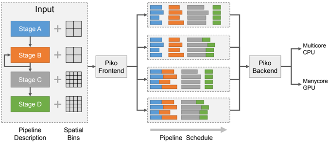
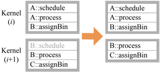
Figure 1: Piko is a framework for designing and implementing programmable graphics pipelines that can be easily retargeted to different application configurations and architectural targets. Piko's input is a functional and structural description of the desired graphics pipeline, augmented with a per-stage grouping of computation into spatial bins (or tiles), and a scheduling preference for these bins. Our compiler generates efficient implementations of the input pipeline for multiple architectures and allows the programmer to tweak these implementations using simple changes in the bin configurations and scheduling preferences.
<details>
<summary>Image 1 Details</summary>
### Visual Description
## Diagram: Piko System Architecture and Pipeline Scheduling
### Overview
This image presents a system diagram illustrating the Piko system, which processes a pipeline description and spatial binning information to generate a pipeline schedule, ultimately targeting different hardware architectures. The diagram is divided into three main conceptual sections: Input, Piko Frontend and Pipeline Schedule, and Piko Backend with its outputs. It shows how a sequential pipeline can be transformed into various parallel schedules.
### Components/Axes
**Left Section: Input**
* **Bounding Box Label**: "Input" (top-center of the dashed box)
* **Pipeline Description**: A vertical sequence of four rectangular blocks, representing stages of a pipeline:
* **Stage A**: Blue rectangle, top.
* **Stage B**: Orange rectangle, second from top. An arrow indicates a feedback loop from the output of Stage C back to the input of Stage B.
* **Stage C**: Grey rectangle, third from top.
* **Stage D**: Green rectangle, bottom.
* **Flow**: Downward arrows connect Stage A to B, B to C, and C to D, indicating sequential execution.
* **Spatial Bins**: To the right of each pipeline stage, a grid icon represents spatial binning:
* **Stage A**: A 2x2 grid (4 cells).
* **Stage B**: A 2x2 grid (4 cells).
* **Stage C**: A 4x4 grid (16 cells).
* **Stage D**: A 4x4 grid (16 cells).
* **Labels below Input section**:
* "Pipeline Description" (bottom-left)
* "Spatial Bins" (bottom-right)
**Middle Section: Piko Frontend and Pipeline Schedule**
* **Piko Frontend**: A grey rectangular block labeled "Piko Frontend", positioned centrally between the Input and Pipeline Schedule sections. An arrow points from the "Input" dashed box to "Piko Frontend".
* **Pipeline Schedule**: Four distinct dashed bounding boxes, arranged vertically, each containing a set of horizontal stacked bar charts. Arrows point from "Piko Frontend" to each of these four schedule boxes, indicating parallel processing or different scheduling options.
* **Axis/Label**: A horizontal grey arrow below these four boxes is labeled "Pipeline Schedule", indicating a timeline or progression.
* **Bar Chart Structure (within each schedule box)**: Each box contains 3 rows of horizontal stacked bars. Each row appears to represent a separate task or thread. Each bar is composed of four colored segments, corresponding to the pipeline stages:
* Blue segment: Stage A
* Orange segment: Stage B
* Grey segment: Stage C
* Green segment: Stage D
**Right Section: Piko Backend and Outputs**
* **Piko Backend**: A grey rectangular block labeled "Piko Backend", positioned centrally to the right of the Pipeline Schedule section. Arrows point from each of the four "Pipeline Schedule" boxes to "Piko Backend".
* **Outputs**: Two output labels with arrows originating from "Piko Backend":
* "Multicore CPU" (top-right)
* "Manycore GPU" (bottom-right)
### Detailed Analysis
**Input Section:**
The input defines a four-stage pipeline (A, B, C, D) with a feedback loop from Stage C to Stage B. Stages A and B operate on a coarser 2x2 spatial binning, while Stages C and D operate on a finer 4x4 spatial binning. This suggests a hierarchical or multi-resolution processing approach.
**Pipeline Schedule Section (Detailed Bar Analysis):**
Each of the four "Pipeline Schedule" blocks shows three horizontal bars, representing three parallel execution units or tasks. The length of each colored segment within a bar indicates the relative duration or workload of that stage for that specific task.
1. **Top Pipeline Schedule Block**:
* **Trend**: All three bars show a predominantly sequential execution of stages A, B, C, and D from left to right.
* **Details**:
* **Bar 1 (Top)**: Blue (A) is short, followed by Orange (B) which is slightly longer, then Grey (C) which is the longest, and Green (D) which is medium length.
* **Bar 2 (Middle)**: Similar to Bar 1, with short Blue (A), slightly longer Orange (B), longest Grey (C), and medium Green (D).
* **Bar 3 (Bottom)**: Similar to Bar 1 and 2, with short Blue (A), slightly longer Orange (B), longest Grey (C), and medium Green (D).
* **Observation**: This schedule appears to be a basic, mostly sequential execution across three parallel tasks, with Stage C consuming the most time.
2. **Second Pipeline Schedule Block (from top)**:
* **Trend**: Similar to the top block, showing sequential execution, but with minor variations in segment lengths and possibly slightly different start times for stages across the tasks.
* **Details**:
* **Bar 1 (Top)**: Blue (A) is short, Orange (B) is slightly longer, Grey (C) is the longest, Green (D) is medium.
* **Bar 2 (Middle)**: Blue (A) is short, Orange (B) is slightly longer, Grey (C) is the longest, Green (D) is medium.
* **Bar 3 (Bottom)**: Blue (A) is short, Orange (B) is slightly longer, Grey (C) is the longest, Green (D) is medium.
* **Observation**: This schedule is very similar to the first, suggesting a baseline or slightly optimized sequential execution.
3. **Third Pipeline Schedule Block (from top)**:
* **Trend**: This block shows significant overlap and parallelization, particularly between Stage A and B, and Stage B and C. The stages are no longer strictly sequential within a single bar.
* **Details**:
* **Bar 1 (Top)**: Blue (A) starts, then Orange (B) starts *before* A finishes, overlapping significantly. Grey (C) starts *before* B finishes, also overlapping. Green (D) starts *before* C finishes, with some overlap.
* **Bar 2 (Middle)**: Similar overlapping pattern as Bar 1, with A, B, C, D segments showing concurrent execution.
* **Bar 3 (Bottom)**: Similar overlapping pattern as Bar 1 and 2.
* **Observation**: This schedule demonstrates pipelining or fine-grained parallelization, where stages begin processing before preceding stages are fully complete, leading to a shorter overall execution time for each task.
4. **Bottom Pipeline Schedule Block**:
* **Trend**: This block continues the trend of the third block, showing extensive overlap and parallelization among stages A, B, C, and D.
* **Details**:
* **Bar 1 (Top)**: Strong overlap between A and B, B and C, and C and D. The total length of the bar (overall task duration) appears shorter than in the first two blocks.
* **Bar 2 (Middle)**: Similar extensive overlapping pattern.
* **Bar 3 (Bottom)**: Similar extensive overlapping pattern.
* **Observation**: This schedule represents a highly optimized, parallel execution, likely leveraging the maximum possible concurrency between pipeline stages.
### Key Observations
* The system takes a "Pipeline Description" (sequential stages with a feedback loop) and "Spatial Bins" (different granularities for stages) as input.
* The "Piko Frontend" transforms this input into various "Pipeline Schedules".
* The "Pipeline Schedule" section demonstrates a progression from mostly sequential execution (top two blocks) to highly parallelized and pipelined execution (bottom two blocks).
* Each schedule block shows three parallel tasks, suggesting the system can schedule multiple instances of the pipeline concurrently.
* The "Piko Backend" takes these schedules and targets them for execution on "Multicore CPU" or "Manycore GPU", implying hardware-specific optimization.
* The feedback loop from Stage C to Stage B in the input pipeline description is a notable feature, suggesting iterative processing or refinement.
* The change in spatial binning from 2x2 to 4x4 between Stage B and C indicates a potential change in data resolution or processing granularity within the pipeline.
### Interpretation
The Piko system appears to be a compiler or runtime system designed to optimize the execution of image processing or data-parallel pipelines.
1. **Input Definition**: The "Input" section defines a computational graph (the pipeline stages) and associated data characteristics (spatial bins). The feedback loop (C to B) suggests an iterative algorithm, possibly for refinement or convergence. The varying spatial bins imply that different stages might operate on different resolutions or data partitions, which is common in image processing (e.g., downsampling, processing, then upsampling).
2. **Frontend's Role**: The "Piko Frontend" likely analyzes this pipeline description and spatial information to identify potential parallelism and dependencies. It then generates different possible execution schedules. The four "Pipeline Schedule" blocks represent different strategies or levels of optimization that the frontend can produce. The progression from sequential to highly parallel schedules demonstrates the frontend's ability to explore the scheduling space.
3. **Scheduling Strategies**:
* The top two schedule blocks show a more conservative, sequential execution, possibly suitable for simpler hardware or when dependencies are strict.
* The bottom two schedule blocks, with their significant overlaps, illustrate aggressive pipelining and parallelization. This suggests that the Piko system can break down stages into smaller, concurrently executable units, or that it can overlap the execution of different stages across different data elements (e.g., processing Stage A for data element 2 while Stage B processes data element 1). This is crucial for maximizing throughput on modern parallel hardware.
4. **Backend's Role and Hardware Targeting**: The "Piko Backend" takes these optimized schedules and translates them into executable code or instructions for specific hardware. The outputs "Multicore CPU" and "Manycore GPU" highlight Piko's capability to target diverse parallel architectures, implying that the backend performs architecture-specific code generation and optimization (e.g., using OpenMP for CPU, CUDA/OpenCL for GPU). The choice of schedule might depend on the target hardware's capabilities and the desired performance characteristics.
In essence, Piko automates the complex task of transforming a high-level, potentially sequential pipeline description into highly optimized, parallel execution schedules tailored for different parallel computing platforms, thereby abstracting away much of the low-level parallel programming effort. The visual representation of varying schedules effectively communicates the system's ability to exploit different levels of parallelism.
</details>
## Abstract
We present Piko, a framework for designing, optimizing, and retargeting implementations of graphics pipelines on multiple architectures. Piko programmers express a graphics pipeline by organizing the computation within each stage into spatial bins and specifying a scheduling preference for these bins. Our compiler, Pikoc , compiles this input into an optimized implementation targeted to a massively-parallel GPU or a multicore CPU.
Piko manages work granularity in a programmable and flexible manner, allowing programmers to build load-balanced parallel pipeline implementations, to exploit spatial and producer-consumer locality in a pipeline implementation, and to explore tradeoffs between these considerations. We demonstrate that Piko can implement a wide range of pipelines, including rasterization, Reyes, ray tracing, rasterization/ray tracing hybrid, and deferred rendering. Piko allows us to implement efficient graphics pipelines with relative ease and to quickly explore design alternatives by modifying the spatial binning configurations and scheduling preferences for individual stages, all while delivering real-time performance that is within a factor six of state-of-the-art rendering systems.
CR Categories: I.3.1 [Computer Graphics]: Hardware architecture-Parallel processing; I.3.2 [Computer Graphics]: Graphics Systems-Stand-alone systems
∗ email:apatney@nvidia.com
† email:stzeng@nvidia.com
‡ email:kaseitz@ucdavis.edu
§ email:jowens@ece.ucdavis.edu
Keywords:
graphics pipelines, parallel computing
## 1 Introduction
Renderers in computer graphics often build upon an underlying graphics pipeline: a series of computational stages that transform a scene description into an output image. Conceptually, graphics pipelines can be represented as a graph with stages as nodes, and the flow of data along directed edges of the graph. While some renderers target the special-purpose hardware pipelines built into graphics processing units (GPUs), such as the OpenGL/Direct3D pipeline (the 'OGL/D3D pipeline'), others use pipelines implemented in software, either on CPUs or, more recently, using the programmable capabilities of modern GPUs. This paper concentrates on the problem of implementing a graphics pipeline that is both highly programmable and high-performance by targeting programmable parallel processors like GPUs.
Hardware implementations of the OGL/D3D pipeline are extremely efficient, and expose programmability through shaders which customize the behavior of stages within the pipeline. However, developers cannot easily customize the structure of the pipeline itself, or the function of non-programmable stages. This limited programmability makes it challenging to use hardware pipelines to implement other types of graphics pipelines, like ray tracing, micropolygon-based pipelines, voxel rendering, volume rendering, and hybrids that incorporate components of multiple pipelines. Instead, developers have recently begun using programmable GPUs to implement these pipelines in software (Section 2), allowing their use in interactive applications.
Efficient implementations of graphics pipelines are complex: they must consider parallelism, load balancing, and locality within the bounds of a restrictive programming model. In general, successful pipeline implementations have been narrowly customized to a particular pipeline and often to a specific hardware target. The abstractions and techniques developed for their implementation are not easily extensible to the more general problem of creating efficient yet structurally- as well as functionally-customizable, or programmable pipelines. Alternatively, researchers have explored more general systems for creating programmable pipelines, but these systems compare poorly in performance against more customized pipelines, primarily because they do not exploit specific characteristics of the pipeline that are necessary for high performance.
Our framework, Piko, builds on spatial bins, or tiles, to expose an interface which allows pipeline implementations to exploit loadbalanced parallelism and both producer-consumer and spatial locality, while still allowing high-level programmability. Like traditional pipelines, a Piko pipeline consists of a series of stages (Figure 1), but we further decompose those stages into three abstract phases (Table 2). These phases expose the salient characteristics of the pipeline that are helpful for achieving high performance. Piko pipelines are compiled into efficient software implementations for multiple target architectures using our compiler, Pikoc . Pikoc uses the LLVM framework [Lattner and Adve 2004] to automatically translate user pipelines into the LLVM intermediate representation (IR) before converting it into code for a target architecture.
We see two major differences from previous work. First, we describe an abstraction and system for designing and implementing generalized programmable pipelines rather than targeting a single programmable pipeline. Second, our abstraction and implementation incorporate spatial binning as a fundamental component, which we demonstrate is a key ingredient of high-performance programmable graphics pipelines.
The key contributions of this paper include:
- Leveraging programmable binning for spatial locality in our abstraction and implementation, which we demonstrate is critical for high performance;
- Factoring pipeline stages into 3 phases, AssignBin , Schedule , and Process , which allows us to flexibly exploit spatial locality and which enhances portability by factoring stages into architecture-specific and -independent components;
- Automatically identifying and exploiting opportunities for compiler optimizations directly from our pipeline descriptions; and
- A compiler at the core of our programming system that automatically and effectively generates pipeline code from the Piko abstraction, achieving our goal of constructing easily-modifiable and -retargetable, high-performance, programmable graphics pipelines.
## 2 Programmable Graphics Abstractions
Historically, graphics pipeline designers have attained flexibility through the use of programmable shading. Beginning with a fixedfunction pipeline with configurable parameters, user programmability began in the form of register combiners, expanded to programmable vertex and fragment shaders (e.g., Cg [Mark et al. 2003]), and today encompasses tessellation, geometry, and even generalized compute shaders in Direct3D 11. Recent research has also proposed programmable hardware stages beyond shading, including a delay stream between the vertex and pixel processing units [Aila et al. 2003] and the programmable culling unit [Hasselgren and Akenine-Möller 2007].
The rise in programmability has led to a number of innovations beyond the OGL/D3D pipeline. Techniques like deferred rendering (including variants like tiled-deferred lighting in compute shaders, as well as subsequent approaches like 'Forward+' and clustered forward rendering), amount to building alternative pipelines that schedule work differently and exploit different trade-offs in locality, parallelism, and so on. In fact, many modern games already implement a deferred version of forward rendering to reduce the cost of shading and reduce the number of rendering passes [Andersson 2009].
Recent research uses the programmable aspects of modern GPUs to implement entire pipelines in software. These efforts include RenderAnts, which implements a GPU Reyes renderer [Zhou et al. 2009]; cudaraster [Laine and Karras 2011], which explores software rasterization on GPUs; VoxelPipe, which targets real-time GPU voxelization [Pantaleoni 2011], and the Micropolis Reyes renderer [Weber et al. 2015]. The popularity of such explorations demonstrates that entirely programmable pipelines are not only feasible but desirable as well. These projects, however, target a single specific pipeline for one specific architecture, and as a consequence their implementations offer limited opportunities for flexibility and reuse.
A third class of recent research seeks to rethink the historical approach to programmability, and is hence most closely related to our work. GRAMPS [Sugerman et al. 2009] introduces a programming model that provides a general set of abstractions for building parallel graphics (and other) applications. Sanchez et al. [2011] implemented a multi-core x86 version of GRAMPS. NVIDIA's high-performance programmable ray tracer OptiX [Parker et al. 2010] also allows arbitrary pipes, albeit with a custom scheduler specifically designed for their GPUs. By and large, GRAMPS addresses expression and scheduling at the level of pipeline organization, but does not focus on handling efficiency concerns within individual stages. Instead, GRAMPS successfully focuses on programmability, heterogeneity, and load balancing, and relies on the efficient design of inter-stage sequential queues to exploit producer-consumer locality. The latter is in itself a challenging implementation task that is not addressed by the GRAMPS abstraction. The principal difference in our work is that instead of using queues, we use 2D tiling to group computation in a manner that helps balance parallelism with locality and is more optimized towards graphcal workloads. While GRAMPS proposes queue sets to possibly expose parallelism within a stage (which may potentially support spatial bins), it does not allow any flexibility in the scheduling strategies for individual bins, which, as we will demonstrate, is important to ensure efficiency by tweaking the balance between spatial/temporal locality and load balance. Piko also merges user stages together into a single kernel for efficiency purposes. GRAMPS relies directly on the programmer's decomposition of work into stages so that fusion, which might be a target-specific optimization, must be done at the level of the input pipeline specification.
Peercy et al. [2000] and FreePipe [Liu et al. 2010] implement an entire OGL/D3D pipeline in software on a GPU, then explore modifications to their pipeline to allow multi-fragment effects. These GPGPU software rendering pipelines are important design points; they describe and analyze optimized GPU-based software implementations of an OGL/D3D pipeline, and are thus important comparison points for our work. We demonstrate that our abstraction allows us to identify and exploit optimization opportunities beyond the FreePipe implementation.
Halide [Ragan-Kelley et al. 2012] is a domain-specific embedded language that permits succinct, high-performance implementations of state-of-the-art image-processing pipelines. In a manner similar to Halide, we hope to map a high-level pipeline description to a lowlevel efficient implementation. However, we employ this strategy in a different application domain, programmable graphics, where data
Table 1: Examples of Binning in Graphics Architectures. We characterize pipelines based on when spatial binning occurs. Pipelines that bin prior to the geometry stage are classified under 'referenceimage binning'. Interleaved and tiled rasterization pipelines typically bin between the geometry and rasterization stage. Tiled depth-based composition pipelines bin at the sample or composition stage. Finally, 'bin everywhere' pipelines bin after every stage by re-distributing the primitives in dynamically updated queues.
| Reference-Image Binning | PixelFlow [Olano and Lastra 1998] Chromium [Humphreys et al. 2002] |
|-------------------------------|------------------------------------------------------------------------------------------------------------------------------------------------------------------------|
| Interleaved Rasterization | AT&T Pixel Machine [Potmesil and Hoffert 1989] SGI InfiniteReality [Montrym et al. 1997] NVIDIA Fermi [Purcell 2010] |
| Tiled Rasterization/ Chunking | RenderMan [Apodaca and Mantle 1990] cudaraster [Laine and Karras 2011] ARMMali [Olson 2012] PowerVR [Imagination Technologies Ltd. 2011] RenderAnts [Zhou et al. 2009] |
| Tiled Depth-Based Composition | Lightning-2 [Stoll et al. 2001] |
| Bin Everywhere | Pomegranate [Eldridge et al. 2000] |
granularity varies much more throughout the pipeline and dataflow is both more dynamically varying and irregular. Spark [Foley and Hanrahan 2011] extends the flexibility of shaders such that instead of being restricted to a single pipeline stage, they can influence several stages across the pipeline. Spark allows such shaders without compromising modularity or having a significant impact on performance, and in fact Spark could be used as a shading language to layer over pipelines created by Piko. We share design goals that include both flexibility and competitive performance in the same spirit as Sequoia [Fatahalian et al. 2006] and StreamIt [Thies et al. 2002] in hopes of abstracting out the computation from the underlying hardware.
## 3 Spatial Binning
Both classical and modern graphics systems often render images by dividing the screen into a set of regions, called tiles or spatial bins , and processing those bins in parallel. Examples include tiled rasterization, texture and framebuffer memory layouts, and hierarchical depth buffers. Exploiting spatial locality through binning has five major advantages. First, it prunes away unnecessary work associated with the bin-primitives not affecting a bin are never processed. Second, it allows the hardware to take advantage of data and execution locality within the bin itself while processing (for example, tiled rasterization leads to better locality in a texture cache). Third, many pipeline stages may have a natural granularity of work that is most efficient for that particular stage; binning allows programmers to achieve this granularity at each stage by tailoring the size of bins. Fourth, it exposes an additional level of data parallelism, the parallelism between bins. And fifth, grouping computation into bins uncovers additional opportunities for exploiting producer-consumer locality by narrowing working-set sizes to the size of a bin.
Spatial binning has been a key part of graphics systems dating to some of the earliest systems. The Reyes pipeline [Cook et al. 1987] tiles the screen, rendering one bin at a time to avoid working sets that are too large; Pixel-Planes 5 [Fuchs et al. 1989] uses spatial binning primarily for increasing parallelism in triangle rendering and other pipelines. More recently, most major GPUs use some form of spatial binning, particularly in rasterization [Olson 2012; Purcell 2010].
Recent software renderers written for CPUs and GPUs also make extensive use of screen-space tiling: RenderAnts [Zhou et al. 2009] uses buckets to limit memory usage during subdivision and sample stages, cudaraster [Laine and Karras 2011] uses a bin hierarchy to eliminate redundant work and provide more parallelism, and VoxelPipe [Pantaleoni 2011] uses tiles for both bucketing purposes and exploiting spatial locality. Table 1 shows examples of graphics systems that have used a variety of spatial binning strategies.
The advantages of spatial binning are so compelling that we believe, and will show, that exploiting spatial binning is a crucial component for performance in efficient implementations of graphics pipelines. Previous work in software-based pipelines that take advantage of binning has focused on specific, hardwired binning choices that are narrowly tailored to one particular pipeline. In contrast, the Piko abstraction encourages pipeline designers to express pipelines and their spatial locality in a more general, flexible, straightforward way that exposes opportunities for binning optimizations and performance gains.
## 4 Expressing Pipelines Using Piko
## 4.1 High-Level Pipeline Abstraction
Graphics algorithms and APIs are typically described as pipelines (directed graphs) of simple stages that compose to create complex behaviors. The OGL/D3D abstraction is described in this fashion, as are Reyes and GRAMPS, for instance. Pipelines aid understanding, make dataflow explicit, expose locality, and permit reuse of individual stages across different pipelines. At a high level, the Piko pipeline abstraction is identical, expressing computation within stages and dataflow as communication between stages. Piko supports complex dataflow patterns, including a single stage feeding input to multiple stages, multiple stages feeding input to a single stage, and cycles (such as Reyes recursive splitting).
Where the abstraction differs is within a pipeline stage. Consider a BASELINE system that would implement one of the above pipelines as a set of separate per-stage kernels, each of which distributes its work to available parallel cores, and the implementation connects the output of one stage to the input of the next through off-chip memory. Each instance of a BASELINE kernel would run over the entire scene's intermediate data, reading its input from off-chip memory and writing its output back to off-chip memory. This implementation would have ordered semantics and distribute work in each stage in FIFO order.
Our BASELINE would end up making poor use of both the producerconsumer locality between stages and the spatial locality within and between stages. It would also require a rewrite of each stage to target a different hardware architecture. Piko specifically addresses these issues by balancing between enabling productivity and portability through a high-level programming model, while specifying enough information to allow high-performance implementations. The distinctive feature of the abstraction is the ability to cleanly separate the implementation of a high-performance graphics pipeline into separable, composable concerns, which provides two main benefits:
- It facilitates modularity and architecture independence.
- It integrates locality and spatial binning in a way that exposes opportunities to explore the space of optimizations involving locality and load-balance.
For the rest of the paper, we will use the following terminology for the parts of a graphics pipeline. Our pipelines are expressed as directed graphs where each node represents a self-contained functional unit or a stage . Edges between nodes indicate flow of data between stages, and each data element that flows through the edges is a primitive . Examples of common primitives are patches, vertices, triangles, and fragments. Stages that have no incoming edges are source stages, and stages with no outgoing edges are drain stages.
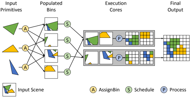
Figure 2: The three phases of a Piko stage. This diagram shows the role of AssignBin , Schedule , and Process in the scan conversion of a list of triangles using two execution cores. Spatial binning helps in (a) extracting load-balanced parallelism by assigning triangles into smaller, more uniform, spatial bins, and (b) preserving spatial locality within each bin by grouping together spatially-local data. The three phases help fine-tune how computation is grouped and scheduled, and this helps quickly explore the optimization space of an implementation.
<details>
<summary>Image 2 Details</summary>
### Visual Description
## Diagram: Geometric Primitive Processing Pipeline
### Overview
This diagram illustrates a multi-stage parallel processing pipeline for geometric primitives, transforming them from individual shapes into a combined rasterized output. The process involves assigning input primitives to spatial bins, scheduling these bins to parallel execution cores, processing the primitives within each core, and finally aggregating the results into a single output grid.
### Components/Axes
The diagram is structured into four main conceptual stages, labeled horizontally from left to right:
1. **Input Primitives**: The initial geometric shapes.
2. **Populated Bins**: Collections of primitives grouped into logical units.
3. **Execution Cores**: Parallel processing units.
4. **Final Output**: The aggregated, rasterized result.
**Legend (located at the bottom of the diagram):**
* **Input Scene**: Represented by a white square containing an overlapping green irregular quadrilateral, a yellow trapezoid, and a blue irregular triangle. This symbol is used to depict the contents of the "Populated Bins" and the inputs to the "Execution Cores".
* **(A) AssignBin**: Represented by a yellow circular node with the letter 'A'. This component is responsible for distributing input primitives to bins.
* **(S) Schedule**: Represented by a green circular node with the letter 'S'. This component is responsible for assigning populated bins to execution cores.
* **(P) Process**: Represented by a blue circular node with the letter 'P'. This component performs the actual processing (e.g., rasterization) of primitives within an execution core.
### Detailed Analysis
**1. Input Primitives (Leftmost Column):**
Three distinct geometric primitives are shown vertically:
* **Top**: A green irregular quadrilateral/pentagon.
* **Middle**: A yellow trapezoid.
* **Bottom**: A blue irregular triangle/quadrilateral.
**2. AssignBin (A) Nodes:**
Three yellow circular 'A' nodes are positioned to the right of the input primitives. Each 'A' node receives an arrow from one input primitive:
* The top 'A' node receives input from the green primitive.
* The middle 'A' node receives input from the yellow primitive.
* The bottom 'A' node receives input from the blue primitive.
Each 'A' node has multiple outgoing arrows connecting to the "Populated Bins", indicating that a single primitive can be assigned to multiple bins.
**3. Populated Bins (Second Column from Left):**
Four white square bins are arranged vertically. Each bin contains a combination of the input primitives, representing an "Input Scene" as per the legend.
* **Bin 1 (Top)**: Contains the majority of the green primitive and a small portion of the blue primitive. It receives input from the top 'A' (green primitive) and the bottom 'A' (blue primitive).
* **Bin 2**: Contains a small portion of the green primitive and a small portion of the yellow primitive. It receives input from the top 'A' (green primitive) and the middle 'A' (yellow primitive).
* **Bin 3**: Contains the majority of the blue primitive and a small portion of the yellow primitive. It receives input from the middle 'A' (yellow primitive) and the bottom 'A' (blue primitive).
* **Bin 4 (Bottom)**: Contains the majority of the yellow primitive. It receives input from the middle 'A' (yellow primitive).
Each bin has an outgoing arrow leading to a "Schedule (S)" node.
**4. Schedule (S) Nodes:**
Four green circular 'S' nodes are positioned to the right of the populated bins. Each 'S' node receives an arrow from one populated bin. These nodes then direct their output to the "Execution Cores" with cross-connections:
* The top 'S' node (from Bin 1) directs its output to the top "Execution Core" (left input scene).
* The second 'S' node (from Bin 2) directs its output to the top "Execution Core" (right input scene).
* The third 'S' node (from Bin 3) directs its output to the bottom "Execution Core" (left input scene).
* The bottom 'S' node (from Bin 4) directs its output to the bottom "Execution Core" (right input scene).
**5. Execution Cores (Third Column from Left):**
Two grey rectangular units represent two parallel execution cores. Each core processes two input scenes and produces two corresponding 4x4 pixel grids.
* **Top Execution Core**:
* **Input Scenes**:
* Left: Contains the green primitive (mostly) and a small part of the blue primitive (from Bin 1).
* Right: Contains a small part of the green primitive and a small part of the yellow primitive (from Bin 2).
* **Process (P) Node**: A blue circular 'P' node is centrally located within the core, indicating the processing step.
* **Output Grids (4x4 pixels)**:
* Left Grid (from left input scene):
* Row 1: 1 blue pixel (bottom-left), 3 white pixels.
* Row 2: 4 green pixels.
* Row 3: 4 green pixels.
* Row 4: 4 green pixels.
* Right Grid (from right input scene):
* Row 1: 4 white pixels.
* Row 2: 4 white pixels.
* Row 3: 1 yellow pixel (bottom-left), 3 white pixels.
* Row 4: 1 green pixel (bottom-left), 3 white pixels.
* **Bottom Execution Core**:
* **Input Scenes**:
* Left: Contains the blue primitive (mostly) and a small part of the yellow primitive (from Bin 3).
* Right: Contains the yellow primitive (mostly) (from Bin 4).
* **Process (P) Node**: A blue circular 'P' node is centrally located within the core.
* **Output Grids (4x4 pixels)**:
* Left Grid (from left input scene):
* Row 1: 4 white pixels.
* Row 2: 4 white pixels.
* Row 3: 1 yellow pixel (bottom-left), 3 white pixels.
* Row 4: 4 blue pixels.
* Right Grid (from right input scene):
* Row 1: 4 white pixels.
* Row 2: 4 white pixels.
* Row 3: 4 white pixels.
* Row 4: 4 yellow pixels.
**6. Final Output (Rightmost Column):**
A single 8x8 pixel grid is shown, representing the combined output from both execution cores. The top 4x8 section is derived from the top core's outputs (left 4x4 and right 4x4 grids concatenated horizontally), and the bottom 4x8 section is derived from the bottom core's outputs.
The combined 8x8 grid is as follows (reading left to right, top to bottom):
* **Row 1**: Blue (1), White (7)
* **Row 2**: Green (4), White (4)
* **Row 3**: Green (4), Yellow (1), White (3)
* **Row 4**: Green (5), White (3)
* **Row 5**: White (8)
* **Row 6**: White (8)
* **Row 7**: Yellow (1), White (7)
* **Row 8**: Blue (4), Yellow (4)
### Key Observations
* **Parallelism**: The diagram clearly depicts parallel processing at multiple stages, with multiple bins and two execution cores operating concurrently.
* **Spatial Partitioning/Binning**: Input primitives are distributed into "bins," which appear to represent spatial regions or subsets of a larger scene. A single primitive can contribute to multiple bins if it overlaps multiple regions.
* **Scheduling**: The "Schedule" step implies a mechanism for distributing workload (bins) efficiently among available "Execution Cores".
* **Rasterization**: The "Process" step within the execution cores transforms vector-like geometric primitives into a rasterized (pixel-based) representation.
* **Color Consistency**: The colors (green, yellow, blue) consistently represent the same underlying primitive throughout the entire pipeline, from input shapes to individual pixels in the final output.
* **Aggregation**: The final output is a composite image formed by combining the rasterized results from the individual execution cores.
### Interpretation
This diagram illustrates a common architecture for processing complex geometric scenes, particularly relevant in computer graphics rendering, simulation, or spatial data analysis.
The data flow suggests the following:
1. **Decomposition**: A complex scene (implied by the "Input Scene" legend and the multiple primitives) is decomposed into smaller, manageable sub-regions or "bins" by the "AssignBin" function. This allows for localized processing. The fact that a single primitive can be assigned to multiple bins indicates that bins likely represent spatial tiles, and primitives are assigned to all tiles they intersect.
2. **Load Balancing/Resource Allocation**: The "Schedule" function acts as a dispatcher, distributing these populated bins to available "Execution Cores". This step is crucial for optimizing performance in a parallel system, ensuring cores are utilized effectively.
3. **Parallel Processing**: The "Execution Cores" perform the core computational work in parallel. Each core takes a subset of the scene (two bins in this example), processes the geometric primitives within those bins (e.g., rasterizing them into pixels), and generates a partial output.
4. **Reconstruction**: The "Final Output" stage demonstrates the reassembly of these partial, rasterized results from the parallel cores into a complete, coherent image.
The pipeline effectively demonstrates how a large computational task (processing a scene with multiple geometric primitives) can be broken down, distributed, processed in parallel, and then reassembled, leading to potentially significant performance gains over a purely sequential approach. The consistent use of color helps to visually trace the contribution of each initial primitive through the various stages of transformation and aggregation.
</details>
Table 2: Purpose and granularity for each of the three phases during each stage. We design these phases to cleanly separate the key steps in a pipeline built around spatial binning. Note: we consider Process a per-bin operation, even though it often operates on a per-primitive basis.
| Phase | Granularity | Purpose |
|-----------|--------------------------|------------------------------------|
| AssignBin | Per-Primitive | How to group computation? |
| Schedule | Per-Bin | When to compute? Where to compute? |
| Process | Per-Bin or Per-primitive | How to compute? |
Programmers divide each Piko pipeline stage into three phases (summarized in Table 2 and Figure 2). The input to a stage is a group or list of primitives, but phases, much like OGL/D3D shaders, are programs that apply to a single input element (e.g., a primitive or bin) or a small group thereof. However, unlike shaders, phases belong in each stage of the pipeline, and provide structural as well as functional information about a stage's computation. The first phase in a stage, AssignBin , specifies how a primitive is mapped to a user-defined bin. The second phase, Schedule , assigns bins to cores. The third phase, Process , performs the actual functional computation for the stage on the primitives in a bin. Allowing the programmer to specify both how primitives are binned and how bins are scheduled onto cores allows Pikoc to take advantage of spatial locality.
Now, if we simply replace n pipeline stages with 3 n simpler phases and invoke our BASELINE implementation, we would gain little benefit from this factorization. Fortunately, we have identified and implemented several high-level optimizations on stages and phases that make this factorization profitable. We describe some of our optimizations in Section 5.
As an example, Listing 1 shows the phases of a very simple fragment shader stage. In the AssignBin stage, each fragment goes into a single bin chosen based on its screen-space position. To maximally exploit the machine parallelism, Schedule requests the runtime to distribute bins in a load-balanced fashion across the machine.
Process then executes a simple pixel shader, since the computation by now is well-distributed across all available cores. For the full source code of this simple raster pipeline, please refer to the supplementary materials. Now, let us describe each phase in more detail.
AssignBin The first step for any incoming primitive is to identify the tile(s) that it may influence or otherwise belongs to. Since this depends on both the tile structure as well as the nature of computation in the stage, the programmer is responsible for mapping primitives to bins. Primitives are put in bins with the assignToBin function that assigns a primitive to a bin. Listing 1 assigns an input fragment f based on its screen-space position.
Schedule The best execution schedule for computation in a pipeline varies with stage, characteristics of the pipeline input, and target architectures. Thus, it is natural to want to customize scheduling preferences in order to retarget a pipeline to a different scenario. Furthermore, many pipelines impose constraints on the observable order in which primitives are processed. In Piko, the programmer explicitly provides such preference and constraints on how bins are scheduled on execution cores. Specifically, once primitives are assigned into bins, the Schedule phase allows the programmer to specify how and when bins are scheduled onto cores. The input to Schedule is a reference to a spatial bin, and the routine can chose to dispatch computation for that bin, and if it does, it can also choose a specific execution core or scheduling preference.
We also recognize two cases of special scheduling constraints in the abstraction: the case where all bins from one stage must complete processing before a subsequent stage can begin, and the case where all primitives from one bin must complete processing before any primitives in that bin can be processed by a subsequent stage. Listing 1 shows an example of a Schedule phase that schedules primitives to cores in a load-balanced fashion.
Because of the variety of scheduling mechanisms and strategies on different architectures, we expect Schedule phases to be the most architecture-dependent of the three. For instance, a manycore GPU implementation may wish to maximize utilization of cores by load balancing its computation, whereas a CPU might choose to schedule in chunks to preserve cache peformance, and hybrid CPU-GPU may wish to preferentially assign some tasks to a particular processor
```
class FragmentShaderStage : public Stage {
// ...
void assignBin(int binID = getBinFrom(f, bin) {
this->assignToBin(f, binID);
}
void schedule(int binID) {
specifySchedule(LOAD_BALANCE);
}
void process(piko_fragment f, int binID) {
cvec3f material = gencvc3f(0.80f, 0.75f, 0.65f);
cvec3f lightvec = normalize(gencvc3f(1.1));
this->emit(f, 0);
}
};
Listing 1: Example Piko routines for a fragment shader pipeline
stage and its corresponding pipeline RasterPipe. In the listing,
blue indicates Piko-specific keywords, purple indicates user-defined
parameters, and red indicates parameters that are not specific to Piko.
```
Listing 1: Example Piko routines for a fragment shader pipeline stage and its corresponding pipeline RasterPipe. In the listing, blue indicates Piko-specific keywords, purple indicates user-defined objects, and sea-green indicates user-defined functions. The template parameters to Stage are, in order: binSizeX, binSizeY, threads per bin, incoming primitive type, and outgoing primitive type. We specify a LoadBalance scheduler to take advantage of the many cores on the GPU.
```
(CPU or GPU).
```
Schedule phases specify not only where computation will take place but also when that computation will be launched. For instance, the programmer may specify dependencies that must be satisfied before launching computation for a bin. For example, an order-independent compositor may only launch on a bin once all its fragments are available, and a fragment shader stage may wait for a sufficiently large batch of fragments to be ready before launching the shading computation. Currently, our implementation Pikoc resolves such constraints by adding barriers between stages, but a future implementation might choose to dynamically resolve such dependencies.
Process While AssignBin defines how primitives are grouped for computation into bins, and Schedule defines where and when that computation takes place, the Process phase defines the typical functional role of the stage. The most natural example for Process is a vertex or fragment shader, but Process could be an intersection test, a depth resolver, a subdivision task, or any other piece of logic that would typically form a standalone stage in a conventional graphics pipeline description. The input to Process is the primitive on which it should operate. Once a primitive is processed and the output is ready, the output is sent to the next stage via the emit keyword. emit takes the output and an ID that specifies the next stage. In the graph analogy of nodes (pipeline stages), the ID tells the current node which edge to traverse down toward the next node. Our notation is that Process emit s from zero to many primitives that are the input to the next stage or stages.
We expect that many Process phases will exhibit data parallelism over the primitives. Thus, by default, the input to Process is a single primitive. However, in some cases, a Process phase may be better implemented using a different type of parallelism or may require access to multiple primitives to work correctly. For these cases, we provide a second version of Process that takes a list of primitives as input. This option allows flexibility in how the phase utilizes parallelism and caching, but it limits our ability to perform pipeline optimizations like kernel fusion (discussed in Section 5.2.1). It is also analogous to the categorization of graphics code into pointwise and groupwise computations, as presented by Foley et al. [2011].
## 4.2 Programming Interface
A developer of a Piko pipeline supplies a pipeline definition with each stage separated into three phases: AssignBin , Schedule , and Process . Pikoc analyzes the code to generate a pipeline skeleton that contains information about the vital flow of the pipeline. From the skeleton, Pikoc performs a synthesis stage where it merges pipeline stages together to output an efficient set of kernels that executes the original pipeline definition. The optimizations performed during synthesis, and different runtime implementations of the Piko kernels, are described in detail in Section 5 and Section 6 respectively.
From the developer's perspective, one writes several pipeline stage definitions; each stage has its own AssignBin , Schedule , and Process . Then the developer writes a pipeline class that connects the pipeline stages together. We express our stages in a simple C++-like language.
These input files are compiled by Pikoc into two files: a file containing the target architecture kernel code, and a header file with a class that connects the kernels to implement the pipeline. The developer creates an object of this class and calls the run() method to run the specified pipeline.
The most important architectural targets for Piko are multi-core CPU architectures and manycore GPUs 1 , and Pikoc is able to generate code for both. In the future we also would like to extend its capabilities to target clusters of CPUs and GPUs, and CPU-GPU hybrid architectures.
## 4.3 Using Directives When Specifying Stages
Pikoc exposes several special keywords, which we call directives , to help a developer directly express commonly-used yet complex implementation preferences. We have found that it is usually best for the developer to explicitly state a particular preference, since it is often much easier to do so, and at the same time it helps enable optimizations which Pikoc might not have gathered using static analysis. For instance, if the developer wishes to broadcast a primitive to all bins in the next stage, he can simply use AssignToAll in AssignBin . Directives act as compiler hints and further increase optimization potential. We summarize our directives in Table 3 and discuss their use in Section 5.
We combine these directives with the information that Pikoc derives in its analysis step to create what we call a pipeline skeleton. The skeleton is the input to Pikoc 's synthesis step, which we also describe in Section 5.
## 4.4 Expressing Common Pipeline Preferences
We now present a few commonly encountered pipeline design strategies, and how we interpret them in our abstraction:
No Tiling In cases where tiling is not a beneficial choice, the simplest way to indicate it in Piko is to set bin sizes of all stages to 0 × 0 ( Pikoc translates it to the screen size). Usually such pipelines (or stages) exhibit parallelism at the per-primitive level. In Piko, we can use All and tileSplitSize in Schedule to specify the size of individual primitive-parallel chunks.
1 In this paper we define a 'core' as a hardware block with an independent program counter rather than a SIMD lane; for instance, an NVIDIA streaming multiprocessor (SM).
Table 3: The list of directives the programmer can specify to Piko during each phase. The directives provide basic structural information about the workflow and facilitate optimizations.
| Phase | Name | Purpose |
|-----------|----------------------------------------------------------------------|-------------------------------------------------------------------------------------------------------------------------------------------------------------------------------------------------------------------------------------------------------------------------------------------------------------------------------------------------------------------------------------------------------------------------------------------|
| AssignBin | AssignPreviousBins AssignToBoundingBox AssignToAll | Assign incoming primitive to the same bin as in the previous stage Assign incoming primitive to bins based on its bounding box Assign incoming primitive to all bins |
| Schedule | DirectMap LoadBalance Serialize All tileSplitSize EndStage(X) EndBin | Statically schedule each bin to available cores in a round-robin fashion Dynamically schedule bins to available cores in a load-balanced fashion Schedule all bins to a single core for sequential execution Schedule a bin to all cores (used with tileSplitSize ) Size of chunks to split a bin across multiple cores (used with All ) Wait until stage X is finished Wait until the previous stage finishes processing the current bin |
Bucketing Renderer Due to resource constraints, often the best way to run a pipeline to completion is through a depth-first processing of bins, that is, running the entire pipeline (or a sequence of stages) over individual bins in serial order. In Piko, it is easy to express this preference through the use of the All directive in Schedule , wherein each bin of a stage maps to all available cores. Our synthesis scheme prioritizes depth-first processing in such scenarios, preferring to complete as many stages for a bin before processing the next bin. See Section 5.2 for details.
Sort-Middle Tiled Renderer A common design methodology for forward renderers divides the pipeline into two phases: world-space geometry processing and screen-space fragment processing. Since Piko allows a different bin size for each stage, we can simply use screen-sized bins with primitive-level parallelism in the geometry phase, and smaller bins for the screen-space processing.
Use of Fixed-Function Hardware Blocks Fixed-function hardware accessible through CUDA or OpenCL (like texture fetch units) is easily integrated into Piko using the mechanisms in those APIs. However, in order to use standalone units like a hardware rasterizer or tessellation unit that cannot be directly addressed, the best way to abstract them in Piko is through a stage that implements a single pass of an OGL/D3D pipeline. For example, a deferred rasterizer could use OGL/D3D for the first stage, then a Piko stage to implement the deferred shading pass.
## 5 Pipeline Synthesis with Pikoc
Pikoc is built on top of the LLVM compiler framework. Since Piko pipelines are written using a subset of C++, Pikoc uses Clang, the C and C++ frontend to LLVM, to compile pipeline source code into LLVMIR. We further use Clang in Pikoc 's analysis step by walking the abstract syntax tree (AST) that Clang generates from the source code. From the AST, we are able to obtain the directives and infer the other optimization information discussed previously, as well as determine how pipeline stages are linked together. Pikoc adds this information to the pipeline skeleton, which summarizes the pipeline and contains all the information necessary for pipeline optimization.
Pikoc then performs pipeline synthesis in three steps. First, we identify the order in which we want to launch individual stages (Section 5.1). Once we have this high-level stage ordering, we optimize the organization of kernels to both maximize producerconsumer locality and eliminate any redundant/unnecessary computation (Section 5.2). The result of this process is the kernel mapping : a scheduled sequence of kernels and the phases that make up the computation inside each. Finally, we use the kernel mapping to output two files that implement the pipeline: the kernel code for the target architecture and a header file that contains host code for setting up and executing the kernel code.
We follow typical convention for building complex applications on GPUs using APIs like OpenCL and CUDA by instantiating a pipeline as a series of kernels. Each kernel represents a machinewide computation consisting of parts of one or more pipeline stages. Rendering each frame consists of launching a sequence of kernels scheduled by a host, or a CPU thread in our case. Neighboring kernel instances do not share local memory, e.g., caches or shared memory.
An alternative to multi-kernel design is to express the entire pipeline as a single kernel, which manages pipeline computation via dynamic work queues and uses a persistent-kernel approach [Aila and Laine 2009; Gupta et al. 2012] to efficiently schedule the computation. This is an attractive strategy for implementation and has been used in OptiX, but we prefer the multi-kernel strategy for two reasons. First, efficient dynamic work-queues are complicated to implement on many core architectures and work best for a single, highly irregular stage. Second, the major advantages of dynamic work queues, including dynamic load balance and the ability to capture producer-consumer locality, are already exposed to our implementation through the optimizations we present in this section.
Currently, Pikoc targets two hardware architectures: multicore CPUs and NVIDIA GPUs. In addition to LLVM's many CPU backends, NVIDIA's libNVVM compiles LLVM IR to PTX assembly code, which can then be executed on NVIDIA GPUs using the CUDA driver API 2 . In the future, Pikoc 's LLVM integration will allow us to easily integrate new back ends (e.g., LLVM backends for SPIR and HSAIL) that will automatically target heterogeneous processors like Intel's Haswell or AMD's Fusion. To integrate a new backend into Pikoc , we also need to map all Piko API functions to their counterparts in the new backend and create a new host code generator that can set up and launch the pipeline on the new target.
## 5.1 Scheduling Pipeline Execution
Given a set of stages arranged in a pipeline, in what order should we run these stages? The Piko philosophy is to use the pipeline skeleton with the programmer-specified directives to build a schedule 3 for these stages. Unlike GRAMPS [Sugerman et al. 2009], which takes a dynamic approach to global scheduling of pipeline stages, we use a largely static global schedule due to our multi-kernel design.
The most straightforward schedule is for a linear, feed-forward pipeline, such as the OGL/D3D rasterization pipeline. In this case,
2 https://developer.nvidia.com/cuda-llvm-compiler
3 Please note that the scheduling described in this section is distinct from the Schedule phase in the Piko abstraction. Scheduling here refers to the order in which we run kernels in a generated Piko pipeline.
we schedule stages in descending order of their distance from the last (drain) stage.
By default, a stage will run to completion before the next stage begins. However, we deviate from this rule in two cases: when we fuse kernels such that multiple stages are part of the same kernel (discussed in Section 5.2.1), and when we launch stages for bins in a depth-first fashion (e.g., chunking), where we prefer to complete an entire bin before beginning another. We generate a depth-first schedule when a stage specification directs the entire machine to operate on a stage's bins in sequential order (e.g., by using the All directive). In this scenario, we continue to launch successive stages for each bin as long as it is possible; we stop when we reach a stage that either has a larger bin size than the current stage or has a dependency that prohibits execution. In other words, when given the choice between launching the same stage on another bin or launching the next stage on the current bin, we choose the latter. This decision is similar to the priorities expressed in Sugerman et al. [2009]. In contrast to GRAMPS, our static schedule prefers launching stages farthest from the drain first, but during any stripmining or depthfirst tile traversal, we prefer stages closer to the drain in the same fashion as the dynamic scheduler in GRAMPS. This heuristic has the following advantage: when multiple branches are feeding into the draining stage, finishing the shorter branches before longer branches runs the risk of over-expanding the state. Launching the stages farthest from the drain ensures that the stages have enough memory to complete their computation.
More complex pipeline graph structures feature branches. With these, we start by partitioning the pipeline into disjoint linear branches, splitting at points of convergence, divergence, or explicit dependency (e.g., EndStage ). This method results in linear, distinct branches with no stage overlap. Within each branch, we order stages using the simple technique described above. However, in order to determine inter-branch execution order, we sort all branches in descending order of the distance-from-drain of the branch's starting stage. We attempt to schedule branches in this order as long as all inter-branch dependencies are contained within the already scheduled branches. If we encounter a branch where this is not true, we skip it until its dependencies are satisfied. Rasterization with a shadow map requires this more complex branch ordering method; the branch of the pipeline that generates the shadow map should be executed before the main rasterization branch.
The final consideration when determining stage execution order is managing pipelines with cycles. For non-cyclic pipelines, we can statically determine stage execution ordering, but cycles create a dynamic aspect because we often do not know at compile time how many times the cycle will execute. For cycles that occur within a single stage (e.g., Reyes's Split in Section 7), we repeatedly launch the same stage until the cycle completes. We acknowledge that launching a single kernel with a dynamic work queue is a better solution in this case, but Pikoc doesn't currently support that. Multi-stage cycles (e.g., the trace loop in a ray tracer) pose a bigger stage ordering challenge. In the case where a stage receives input from multiple stages, at least one of which is not part of a cycle containing the current stage, we allow the current stage to execute (as long as any other dependencies have been met). Furthermore, by identifying the stages that loop back to previously executed stages, we can explicitly determine which portions of the pipeline should be repeated.
Please refer to the supplementary material for some example pipelines and their stage execution order.
## 5.2 Pipeline Optimizations
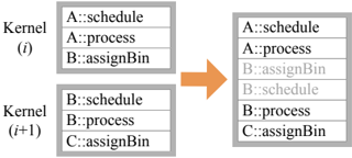
The next step in generating the kernel mapping for a pipeline is determining the contents of each kernel. We begin with a basic, conservative division of stage phases into kernels such that each kernel contains three phases: the current stage's Schedule and Process phases, and the next stage's AssignBin phase. This structure realizes the simple, inefficient BASELINE in which each kernel fetches its bins, schedules them onto cores per Schedule , executes Process on them, and writes the output to the next stage's bins using the latter's AssignBin . The purpose of Pikoc 's optimization step is to use static analysis and programmer-specified directives to find architecture-independent optimization opportunities. We discuss these optimizations below.
## 5.2.1 Kernel Fusion
Combining two kernels into one-'kernel fusion'-both reduces kernel overhead and allows an implementation to exploit producerconsumer locality between the kernels.
<details>
<summary>Image 3 Details</summary>
### Visual Description
## Diagram: Kernel State Merging and Consolidation
### Overview
This image is a diagram illustrating the process of merging or consolidating operations/states from two sequential kernel versions, labeled "Kernel (i)" and "Kernel (i+1)", into a single, combined list. The diagram highlights which operations remain active (black text) and which are potentially superseded or inactive (light gray text) in the merged view.
### Components/Axes
The diagram consists of three main rectangular blocks, each containing a list of text entries, and a large orange arrow connecting the left-side blocks to the right-side block.
* **Left-Top Block:** Labeled "Kernel (i)" on its left side.
* It contains three lines of black text:
* "A::schedule"
* "A::process"
* "B::assignBin"
* **Left-Bottom Block:** Labeled "Kernel (i+1)" on its left side, positioned directly below the "Kernel (i)" block.
* It contains three lines of black text:
* "B::schedule"
* "B::process"
* "C::assignBin"
* **Central Arrow:** A thick, right-pointing orange arrow is positioned to the right of the two "Kernel" blocks, indicating a transformation or merging process.
* **Right Block:** A single, larger rectangular block positioned to the right of the arrow. This block represents the result of the merging process.
* It contains six lines of text, some in black and some in light gray:
* "A::schedule" (black text)
* "A::process" (black text)
* "B::assignBin" (light gray text)
* "B::schedule" (light gray text)
* "B::process" (black text)
* "C::assignBin" (black text)
### Detailed Analysis
The diagram visually represents a consolidation of operations or states from two distinct kernel versions.
1. **Kernel (i) Operations:** The first kernel version includes operations related to components 'A' and 'B'. Specifically, it lists "A::schedule", "A::process", and "B::assignBin".
2. **Kernel (i+1) Operations:** The subsequent kernel version includes operations related to components 'B' and 'C'. Specifically, it lists "B::schedule", "B::process", and "C::assignBin".
3. **Merged List:** The orange arrow signifies a process that combines the operations from "Kernel (i)" and "Kernel (i+1)" into a single, ordered list in the right block. The order of items in the merged list appears to be a direct concatenation, with all items from "Kernel (i)" listed first, followed by all items from "Kernel (i+1)".
* The first two items, "A::schedule" and "A::process", originate from "Kernel (i)" and are displayed in black text.
* The third item, "B::assignBin", also originates from "Kernel (i)" but is displayed in light gray text.
* The fourth item, "B::schedule", originates from "Kernel (i+1)" and is displayed in light gray text.
* The fifth item, "B::process", originates from "Kernel (i+1)" and is displayed in black text.
* The sixth item, "C::assignBin", originates from "Kernel (i+1)" and is displayed in black text.
### Key Observations
* The right block is a union of all unique operations/states present in both Kernel (i) and Kernel (i+1).
* The ordering in the merged list is sequential: all items from Kernel (i) first, then all items from Kernel (i+1).
* The use of light gray text for some entries in the merged list is a key visual cue, indicating a distinction from the black text entries.
* For component 'A', operations "A::schedule" and "A::process" are present only in Kernel (i) and appear in black in the merged list.
* For component 'C', operation "C::assignBin" is present only in Kernel (i+1) and appears in black in the merged list.
* For component 'B', operations are present in both kernels: "B::assignBin" in Kernel (i), and "B::schedule" and "B::process" in Kernel (i+1). In the merged list, "B::assignBin" (from Kernel (i)) and "B::schedule" (from Kernel (i+1)) are gray, while "B::process" (from Kernel (i+1)) is black.
### Interpretation
This diagram likely illustrates a mechanism for managing or tracking operations/states across different versions or iterations of a system, possibly within a kernel or a software component.
The graying out of certain entries in the merged list suggests that these operations or states are either:
1. **Superseded/Inactive:** They are present in the historical record (Kernel (i)) or even the current kernel (Kernel (i+1)), but are no longer the primary or active state for that component in the combined, current view. For instance, "B::assignBin" from Kernel (i) is gray, implying it's superseded by a newer 'B' operation.
2. **Less Significant/Intermediate:** In the case of component 'B', both "B::schedule" and "B::process" are from Kernel (i+1). "B::schedule" is gray, while "B::process" is black. This could imply that "B::process" represents the final or most critical state/operation for component 'B' in Kernel (i+1), while "B::schedule" might be an intermediate step or a less active aspect.
3. **Historical Context:** The merged list provides a comprehensive view of all operations, with the gray text serving to differentiate between currently active/primary operations and those that are historical or less relevant in the current consolidated context.
The overall process demonstrates how a system might maintain a consolidated view of its components' states or operations across iterations, distinguishing between what is currently active and what has been superseded or is of secondary importance. This could be relevant in areas like dependency management, state tracking in concurrent systems, or version control for system components. The diagram effectively communicates a transition or consolidation logic where the most recent and active states are prioritized (black text), while older or less active states are retained for context but visually de-emphasized (gray text).
</details>
Opportunity The simplest case for kernel fusion is when two subsequent stages (a) have the same bin size, (b) map primitives to the same bins, (c) have no dependencies between them, (d) each receive input from only one stage and output to only one stage, and (e) both have Schedule phases that map execution to the same core. For example, a rasterization pipeline's Fragment Shading and Depth Test stages can be fused. If requirements are met, a primitive can proceed from one stage to the next immediately and trivially, so we fuse these two stages into one kernel. These constraints can be relaxed in certain cases (such as a EndBin dependency, discussed below), allowing for more kernel fusion opportunities. We anticipate more complicated cases where kernel fusion is possible but difficult to detect; however, even detecting only the simple case above is highly profitable.
Implementation Two stages, A and B, can be fused by having A's emit statements call B's process phase directly. We can also fuse more than two stages using the same approach.
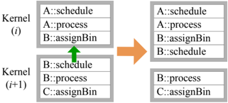
## 5.2.2 Schedule Optimization
While we allow a user to express arbitrary logic in a Schedule routine, we observe that most common patterns of scheduler design can be reduced to simpler and more efficient versions. Two prominent cases include:
## Pre-Scheduling
<details>
<summary>Image 4 Details</summary>
### Visual Description
## Diagram: Kernel State Transformation
### Overview
This diagram illustrates a transformation process involving two distinct kernel states, labeled "Kernel (i)" and "Kernel (i+1)", which represent sequential or related execution contexts. The diagram shows the contents of these kernels before and after a specific operation, highlighting the movement of one particular item from "Kernel (i+1)" to "Kernel (i)". An internal dependency or interaction within the initial state is also depicted.
### Components/Axes
The diagram is structured into two main vertical columns, representing the "before" and "after" states of the kernels, separated by a large horizontal orange arrow indicating the transformation. Each kernel state is represented by a grey-bordered rectangular block containing a list of textual items.
**Left Column (Before Transformation):**
* **Top Block:** Labeled "Kernel (i)" on its left side. This block contains three items, listed vertically:
* "A::schedule"
* "A::process"
* "B::assignBin"
* **Bottom Block:** Labeled "Kernel (i+1)" on its left side. This block contains three items, listed vertically:
* "B::schedule"
* "B::process"
* "C::assignBin"
* **Green Upward Arrow:** A green arrow originates from the "B::schedule" item within the "Kernel (i+1)" block and points upwards to the "B::assignBin" item within the "Kernel (i)" block. This arrow indicates a relationship or flow from "B::schedule" in Kernel (i+1) to "B::assignBin" in Kernel (i).
**Right Column (After Transformation):**
* **Top Block:** This block, corresponding to the transformed "Kernel (i)", contains four items, listed vertically:
* "A::schedule"
* "A::process"
* "B::assignBin"
* "B::schedule"
* **Bottom Block:** This block, corresponding to the transformed "Kernel (i+1)", contains two items, listed vertically:
* "B::process"
* "C::assignBin"
**Transformation Indicator:**
* **Orange Rightward Arrow:** A large, thick orange arrow is positioned horizontally in the center of the diagram, pointing from the left column (before state) to the right column (after state). This signifies the overall transformation or transition.
### Detailed Analysis
**Initial State (Left Column):**
* **Kernel (i):** Contains tasks "A::schedule", "A::process", and "B::assignBin". These appear to be operations or functions prefixed by a module or component identifier (A or B).
* **Kernel (i+1):** Contains tasks "B::schedule", "B::process", and "C::assignBin".
* **Inter-kernel Relationship:** The green arrow explicitly shows a connection where "B::schedule" from Kernel (i+1) is directed towards "B::assignBin" in Kernel (i).
**Transformation (Orange Arrow):**
The orange arrow indicates a change from the initial state to the final state.
**Final State (Right Column):**
* **Transformed Kernel (i):** The contents have changed. It now includes all the original items from Kernel (i) ("A::schedule", "A::process", "B::assignBin") PLUS the item "B::schedule" which was originally in Kernel (i+1).
* **Transformed Kernel (i+1):** The contents have changed. It now contains only "B::process" and "C::assignBin". The item "B::schedule" is no longer present in this kernel.
### Key Observations
1. **Item Movement:** The primary change observed is the movement of the item "B::schedule" from "Kernel (i+1)" to "Kernel (i)".
2. **Kernel (i) Expansion:** "Kernel (i)" gains an item, increasing its task list from three to four.
3. **Kernel (i+1) Contraction:** "Kernel (i+1)" loses an item, decreasing its task list from three to two.
4. **Stable Items:** "A::schedule", "A::process", "B::assignBin" (in Kernel i) and "B::process", "C::assignBin" (in Kernel i+1) remain in their respective kernels, though "B::assignBin" in Kernel (i) is the target of the green arrow.
5. **Green Arrow Context:** The green arrow, originating from the item that moves, and pointing to an item in the destination kernel, suggests a dependency or a reason for the movement.
### Interpretation
This diagram illustrates a mechanism for task or operation migration between sequential kernel states. The "Kernel (i)" and "Kernel (i+1)" likely represent different phases, iterations, or levels of execution within a system.
The core idea is that a task, "B::schedule", initially designated for a later kernel state (i+1), is "pulled" or "promoted" into an earlier kernel state (i). This could be driven by several factors:
* **Dependency Resolution:** The green arrow from "B::schedule" (in i+1) to "B::assignBin" (in i) strongly suggests that "B::schedule" might be a prerequisite or a closely related operation that needs to be executed within the context of "Kernel (i)", possibly before or in conjunction with "B::assignBin". To satisfy this dependency, "B::schedule" is moved.
* **Optimization/Scheduling:** Moving "B::schedule" earlier might be an optimization to improve performance, reduce latency, or ensure critical tasks are handled sooner.
* **Contextual Shift:** The task "B::schedule" might be more relevant or efficient to execute within the environment or resources available to "Kernel (i)" rather than "Kernel (i+1)".
* **Dynamic Reconfiguration:** The diagram could represent a dynamic reconfiguration of kernel tasks based on runtime conditions or specific system requirements.
The "A::" and "C::" prefixed tasks, along with "B::process", remain static, indicating that this specific transformation targets only "B::schedule" and its relationship with "B::assignBin". This suggests a fine-grained control over task placement and execution order across kernel states. The diagram effectively visualizes a "task hoisting" or "pre-scheduling" operation.
</details>
Opportunity For many Schedule phases, core selection is either static or deterministic given the incoming bin ID (specifically, when DirectMap , Serialize , or All are used). In these scenarios, we can pre-calculate the target core ID even before Schedule is ready for execution (i.e., before all dependencies have been met). This both eliminates some runtime work and provides the opportunity to run certain tasks (such as data allocation on heterogeneous implementations) before a stage is ready to execute.
Implementation The optimizer detects the pre-scheduling optimization by identifying one of the three aforementioned Schedule directives. This optimization allows us to move a given stage's Schedule phase into the same kernel as its AssignBin phase so that core selection happens sooner and so that other implementationspecific benefits can be exploited.
## Schedule Elimination
<details>
<summary>Image 5 Details</summary>
### Visual Description
## Diagram: Kernel State Transformation
### Overview
This image presents a diagram illustrating a transformation or filtering process applied to two distinct kernel states, labeled "Kernel (i)" and "Kernel (i+1)". The diagram shows the initial state on the left, an orange arrow indicating a transition, and the resulting state on the right. Each kernel state is represented by a rectangular block containing a list of items, likely representing functions, processes, or components within that kernel.
### Components/Axes
The diagram is structured into two main columns and two rows, with an arrow in the center column indicating a transformation from left to right.
* **Left Column (Initial State):**
* **Top-left block:** Labeled "Kernel (i)" on its left side. This block contains three text entries, each on a new line, within a gray-bordered rectangle.
* **Bottom-left block:** Labeled "Kernel (i+1)" on its left side. This block also contains three text entries within a gray-bordered rectangle, similar in structure to the top-left block.
* **Center Column:**
* An orange, right-pointing arrow is positioned centrally between the left and right columns, spanning both rows.
* **Right Column (Transformed State):**
* **Top-right block:** A gray-bordered rectangle containing three text entries.
* **Bottom-right block:** A gray-bordered rectangle containing two text entries.
### Detailed Analysis
The content of each block is as follows:
* **Kernel (i) - Initial State (Top-left block):**
* A::schedule
* A::process
* B::assignBin
* **Kernel (i+1) - Initial State (Bottom-left block):**
* B::schedule (This text is rendered in a light gray color, distinct from the black text of other entries.)
* B::process
* C::assignBin
* **Transformed State (Top-right block):**
* A::schedule
* A::process
* B::assignBin
(This block is identical in content to the "Kernel (i) - Initial State" block.)
* **Transformed State (Bottom-right block):**
* B::process
* C::assignBin
(This block shows a change from the "Kernel (i+1) - Initial State" block.)
### Key Observations
1. **Kernel (i) Stability:** The content of the "Kernel (i)" block remains entirely unchanged after the transformation. The list "A::schedule", "A::process", "B::assignBin" is present on both the left and right sides for this kernel state.
2. **Kernel (i+1) Modification:** The content of the "Kernel (i+1)" block undergoes a specific change. The entry "B::schedule", which was rendered in light gray text in the initial state, is absent in the transformed state. The other two entries, "B::process" and "C::assignBin", remain present and unchanged.
3. **Significance of Gray Text:** The light gray rendering of "B::schedule" in the initial "Kernel (i+1)" state strongly suggests that this item is a candidate for removal, a temporary element, or an item with a specific status that leads to its exclusion in the subsequent state.
### Interpretation
This diagram illustrates a process of filtering or refinement applied to kernel states. The orange arrow signifies a transition from an initial set of components/tasks to a refined set.
The primary insight is that certain elements, specifically those marked with a distinct visual cue (light gray text), are removed during this transformation. In the context of "Kernel (i+1)", "B::schedule" is identified as an element that does not persist in the transformed state. This could represent:
* **Optimization:** "B::schedule" might be a redundant, unnecessary, or temporary scheduling task that is optimized out.
* **Filtering:** The process might be filtering out specific types of operations or components based on certain criteria, with "B::schedule" meeting those criteria for removal.
* **State Progression:** The transition from Kernel (i) to Kernel (i+1) might involve different sets of operations, and the transformation shown could be a cleanup step for Kernel (i+1) specifically.
The fact that "Kernel (i)" remains entirely unchanged suggests that either the transformation process is not applicable to "Kernel (i)"'s components, or its components are all considered essential and not subject to this particular filtering rule. The diagram effectively highlights a selective removal mechanism, where the visual distinction of "B::schedule" in the initial state provides a strong hint about its fate in the subsequent state.
</details>
Opportunity Modern parallel architectures often support a highly efficient hardware scheduler that offers a reasonably fair allocation of work to computational cores. Despite the limited customizability of such a scheduler, we utilize its capabilities whenever it matches a pipeline's requirements. For instance, if a designer requests bins of a fragment shader to be scheduled in a load-balanced fashion (e.g., using the LoadBalance directive), we can simply offload this task to the hardware scheduler by presenting each bin as an independent unit of work (e.g., a CUDA block or OpenCL workgroup).
Implementation When the optimizer identifies a stage using the LoadBalance directive, it removes that stage's Schedule phase in favor of letting the hardware scheduler allocate the workload.
## 5.2.3 Static Dependency Resolution
<details>
<summary>Image 6 Details</summary>
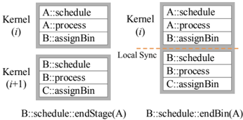
### Visual Description
## Diagram: Kernel Synchronization Comparison
### Overview
This image is a technical diagram illustrating two different approaches to managing kernel operations across consecutive iterations, `Kernel (i)` and `Kernel (i+1)`. It compares a scenario where kernel operations are distinct and separated (left side) with a scenario where they are integrated through a "Local Sync" mechanism (right side), highlighting the impact on specific scheduling events.
### Components/Labels
The diagram is structured into two main vertical sections, left and right, each depicting a different operational model.
**Left Section:**
* **Top Block:** Labeled "Kernel (i)" on its left side. This block has a light grey background and a dark grey border, containing three lines of text:
* "A::schedule"
* "A::process"
* "B::assignBin"
* **Bottom Block:** Labeled "Kernel (i+1)" on its left side. This block also has a light grey background and a dark grey border, positioned directly below the "Kernel (i)" block. It contains three lines of text:
* "B::schedule"
* "B::process"
* "C::assignBin"
* **Bottom Text (Left):** Located below the "Kernel (i+1)" block, the text reads: "B::schedule::endStage(A)"
**Right Section:**
* **Combined Block:** This section features a single, taller block with a light grey background and a dark grey border, vertically divided by a dashed orange line.
* **Label:** "Kernel (i)" is positioned to the left of the upper part of this combined block, at the same vertical level as the "Kernel (i)" label on the left side.
* **Upper Part Content:** Contains the same three lines of text as the "Kernel (i)" block on the left:
* "A::schedule"
* "A::process"
* "B::assignBin"
* **Separator:** A dashed orange horizontal line separates the upper and lower parts of the combined block.
* **Separator Label:** "Local Sync" is positioned to the left of the dashed orange line.
* **Lower Part Content:** Contains the same three lines of text as the "Kernel (i+1)" block on the left:
* "B::schedule"
* "B::process"
* "C::assignBin"
* **Bottom Text (Right):** Located below the combined block, the text reads: "B::schedule::endBin(A)"
### Detailed Analysis
The diagram presents two distinct states or execution models.
**Left Side (Separate Kernels):**
This side shows `Kernel (i)` and `Kernel (i+1)` as two distinct, sequential execution units.
* `Kernel (i)` executes tasks `A::schedule`, `A::process`, and `B::assignBin`.
* Following `Kernel (i)`, `Kernel (i+1)` executes tasks `B::schedule`, `B::process`, and `C::assignBin`.
* The event associated with this model is `B::schedule::endStage(A)`, suggesting that the `B::schedule` operation completes a "stage" related to `A` in this sequential or coarse-grained synchronization model.
**Right Side (Local Sync):**
This side shows `Kernel (i)` and `Kernel (i+1)` operations integrated into a single, continuous block, facilitated by a "Local Sync".
* The upper part of the block, implicitly `Kernel (i)`, contains `A::schedule`, `A::process`, and `B::assignBin`.
* A "Local Sync" operation, indicated by the dashed orange line, occurs after `B::assignBin` from `Kernel (i)`.
* Immediately following the "Local Sync", the lower part of the block, implicitly `Kernel (i+1)`, begins executing `B::schedule`, `B::process`, and `C::assignBin`.
* The event associated with this model is `B::schedule::endBin(A)`, suggesting that the `B::schedule` operation completes a "bin" related to `A` under this local synchronization model.
### Key Observations
* The content of the kernel operations (`A::schedule`, `A::process`, `B::assignBin`, `B::schedule`, `B::process`, `C::assignBin`) remains identical in both scenarios.
* The primary structural difference is the explicit separation of `Kernel (i)` and `Kernel (i+1)` on the left versus their integration via a "Local Sync" on the right.
* The "Local Sync" on the right side effectively merges the execution contexts of `Kernel (i)` and `Kernel (i+1)` into a single, continuous flow, with a synchronization point in between.
* The associated event changes from `B::schedule::endStage(A)` in the separated model to `B::schedule::endBin(A)` in the local sync model. This indicates a change in the granularity or type of completion event for `B::schedule` with respect to `A`.
### Interpretation
This diagram illustrates a conceptual shift in how kernel operations across different iterations (`i` and `i+1`) are synchronized and managed.
The **left side** represents a more traditional or coarse-grained approach. `Kernel (i)` completes all its tasks, and then `Kernel (i+1)` begins. The event `B::schedule::endStage(A)` suggests that the `B::schedule` operation, when it eventually runs in `Kernel (i+1)`, marks the completion of a larger "stage" that might encompass all operations related to `A` from `Kernel (i)` and potentially other preceding tasks. This implies a full barrier or global synchronization between kernel iterations.
The **right side** introduces a "Local Sync" mechanism. This suggests an optimization where the boundary between `Kernel (i)` and `Kernel (i+1)` is not a full global barrier but a more localized synchronization point. After `B::assignBin` from `Kernel (i)`, a "Local Sync" occurs, allowing `B::schedule` from `Kernel (i+1)` to begin immediately. The change in the associated event to `B::schedule::endBin(A)` is crucial. It implies that with "Local Sync", `B::schedule` can complete a smaller, more granular unit of work, a "bin," related to `A`, rather than waiting for a full "stage" to conclude. This could lead to:
* **Improved Latency:** Tasks from `Kernel (i+1)` can start sooner, without waiting for the entire `Kernel (i)` to finish.
* **Better Resource Utilization:** Resources might be released and re-allocated more quickly, or tasks can be pipelined more effectively.
* **Finer-grained Control:** The "Local Sync" allows for more precise control over dependencies between specific tasks across kernel iterations.
In essence, the diagram demonstrates how a "Local Sync" can transform a sequential, stage-based execution model into a more integrated, bin-based execution model, likely for performance or efficiency gains in a system where `Kernel (i)` and `Kernel (i+1)` represent successive computational steps. The specific functions `A::schedule`, `A::process`, `B::assignBin`, `B::schedule`, `B::process`, and `C::assignBin` represent abstract operations within these kernels, and their interaction with `A` and `B` highlights the dependencies being managed.
</details>
Opportunity The previous optimizations allowed us to statically resolve core assignment. Here we also optimize for static resolution of dependencies. The simplest form of dependencies are those that request completion of an upstream stage (e.g., the EndStage directive) or the completion of a bin from the previous stage (e.g., the EndBin directive). The former dependency occurs in rasterization pipelines with shadow mapping, where the Fragment Shade stage cannot proceed until the pipeline has finished generating the shadow map (specifically, the shadow map's Composite stage). The latter dependency occurs when synchronization is required between two stages, but the requirement is spatially localized (e.g., between the Depth Test and Composite stages in a rasterization pipeline with order-independent transparency).
Implementation We interpret EndStage as a global synchronization construct and, thus, prohibit any kernel fusion with a previous stage. By placing a kernel break between stages, we enforce the EndStage dependency because once a kernel has finished running, the stage(s) associated with that kernel are complete.
In contrast, EndBin denotes a local synchronization, so we allow kernel fusion and place a local synchronization within the kernel between stages. However, this strategy only works if a bin is not split across multiple cores. If a bin is split, we fall back to global synchronization.
## 5.2.4 Single-Stage Process Optimizations
Currently, we treat Process stages as architecture-independent. In general, this is a reasonable assumption for graphics pipelines. However, we have noted some specific scenarios where architecturedependent Process routines might be desirable. For instance, with sufficient local storage and small enough bins, a particular architecture might be able to instantiate an on-chip depth buffer, or with a fast global read-only storage, lookup-table-based rasterizers become possible. Exploring architecture-dependent Process stages is an interesting area of future work.
## 6 Runtime Implementation
We designed Piko to target multiple architectures, and we currently focus on two distinct targets: a multicore CPU and a manycore GPU. Certain aspects of our runtime design span both architectures. The uniformity in these decisions provides a good context for comparing differences between the two architectures. The degree of impact of optimizations in Section 5.2 generally varies between architectures, and that helps us tweak pipeline specifications to exploit architectural strengths. Along with using multi-kernel implementations, our runtimes also share the following characteristics:
Bin Management For both architectures, we consider a simple data structure for storing bins: each stage maintains a list of bins, each of which is a list of primitives belonging to the corresponding bin. Currently, both runtimes use atomic operations to read and write to bins. However, using prefix sums for updating bins while maintaining primitive order is a potentially interesting alternative.
Work-Group Organization In order to accommodate the most common scheduling directives of static and dynamic load balance, we simply package execution work groups into CPU threads/CUDA blocks such that they respect the directives we described in Section 4.3:
LoadBalance As discussed in Section 5.2.2, for dynamic load balancing Pikoc simply relies on the hardware scheduler for fair allocation of work. Each bin is assigned to exactly one CPU thread/CUDA block, which is then scheduled for execution by the hardware scheduler.
DirectMap While we cannot guarantee that a specific computation will run on a specific hardware core, here Pikoc packages multiple pieces of computation-for example, multiple binstogether as a single unit to ensure that they will all run on the same physical core.
Piko is designed to target multiple architectures by primarily changing the implementation of the Schedule phase of stages. Due to the intrinsic architectural differences between different hardware targets, the Piko runtime implementation for each target must exploit the unique architectural characteristics of that target in order to obtain efficient pipeline implementations. Below are some architecturespecific runtime implementation details.
Multicore CPU In the most common case, a bin will be assigned to a single CPU thread. When this mapping occurs, we can manage the bins without using atomic operations. Each bin will then be processed serially by the CPU thread.
Generally, we tend to prefer DirectMap Schedule s. This scheduling directive often preserves producer-consumer locality by mapping corresponding bins in different stages to the same hardware core. Today's powerful CPU cache hierarchies allow us to better exploit this locality.
NVIDIA GPU High-end discrete GPUs have a large number of wide-SIMD cores. We thus prioritize supplying large amounts of work to the GPU and ensuring that work is relatively uniform. In specifying our pipelines, we generally prefer Schedule s that use the efficient, hardware-assisted LoadBalance directive whenever appropriate.
Because we expose a threads-per-bin choice to the user when defining a stage, the user can exploit knowledge of the pipeline and/or expected primitive distribution to maximize efficiency. For example, if the user expects many bins to have few primitives in them, then the user can specify a small value for threads-per-bin so that multiple bins get mapped to the same GPU core. This way, we are able to exploit locality within a single bin, but at the same time we avoid losing performance when bins do not have a large number of primitives.
## 7 Evaluation
## 7.1 Piko Pipeline Implementations
In this section, we evaluate performance for two specific pipeline implementations, described below-rasterization and Reyes-but the Piko abstraction can effectively express a range of other pipelines as well. In the supplementary material, we describe several additional Piko pipelines, including a triangle rasterization pipeline with deferred shading, a particle renderer, and and a ray tracer.
BASELINE Rasterizer To understand how one can use Piko to design an efficient graphics pipeline, we begin by presenting a Piko implementation of our BASELINE triangle rasterizer. This pipeline consist of 5 stages connected linearly: Vertex Shader , Rasterizer , Fragment Shader , Depth Test , and Composite . Each of these stages will use full-screen bins, which means that they will not make use of spatial binning. The Schedule phase for each stage will request a LoadBalance scheduler, which will result in each stage being mapped to its own kernel. Thus, we are left with a rasterizer that runs each stage, one-at-a-time, to completion and makes use of neither spatial nor producer-consumer locality. When we run this naive pipeline implementation, the performance leaves much to be desired. We will see how we can improve performance using Piko optimizations in Section 7.2.
Reyes As another example pipeline, let us explore a Piko implementation of a Reyes micropolygon renderer. For our implementation, we split the rendering into four pipeline stages: Split , Dice , Sample , and Shade . One of the biggest differences between Reyes and a forward raster pipeline is that the Split stage in Reyes is irregular in both execution and data. Bezier patches may go through an unbounded number of splits; each split may emit primitives that must be split again ( Split ), or instead diced ( Dice ). These irregularities combined make Reyes difficult to implement efficiently on a GPU. Previous GPU implementations of Reyes required significant amounts of low-level, processor-specific code, such as a custom software scheduler [Patney and Owens 2008; Zhou et al. 2009; Tzeng et al. 2010; Weber et al. 2015].
In contrast, we represent Split in Piko with only a few lines of code. Split is a self-loop stage with two output channels: one back to itself, and the other to Dice . Split 's Schedule stage performs the
Figure 3: We use the above scenes for evaluating characteristics of our rasterizer implementations. Fairy Forest (top-left) is a scene with 174K triangles with many small and large triangles. Buddha (topright) is a scene with 1.1M very small triangles. Mecha (bottom-left) has 254K small- to medium-sized triangles, and Dragon (bottomright) contains 871K small triangles. All tests were performed at a resolution of 1024 × 768.
<details>
<summary>Image 7 Details</summary>
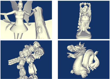
### Visual Description
## 3D Renderings: Collection of Character and Object Models
### Overview
This image displays a grid of four distinct 3D rendered models, each presented in a separate quadrant. The models appear to be computer-generated, showcasing various character types and objects, rendered with a smooth, untextured, monochromatic (light grey/white) surface and distinct lighting, against either a simple two-tone background or a solid dark blue background. The purpose seems to be to highlight the geometric detail and form of the models.
### Image Sections
The image is divided into four approximately equal-sized quadrants, each containing a unique 3D render:
- **Top-Left Quadrant:** Features a fairy-like character alongside a tree trunk.
- **Top-Right Quadrant:** Features a statue of a figure standing on a pedestal.
- **Bottom-Left Quadrant:** Features a robotic mech.
- **Bottom-Right Quadrant:** Features a dragon.
### Detailed Analysis
#### Top-Left Quadrant: Fairy and Tree Trunk
This section displays a light-colored 3D model of a slender, humanoid female figure, resembling a fairy. She has large, delicate wings on her back, a fitted top, and a short, flared skirt. Her hair is styled upwards, and her arms are outstretched. In her left hand, she holds a small, elongated insect with visible wings and a segmented body, possibly a dragonfly or bee. Her right arm is extended towards a roughly cylindrical, light-colored object resembling a tree trunk, which features an oval-shaped indentation or hole on its visible side. The background behind the fairy and tree trunk is split horizontally: the lower portion is a light cream/yellowish color, suggesting ground, while the upper portion is a solid dark blue, suggesting a sky. The models are rendered with smooth surfaces and soft shadows, indicating a focus on form rather than detailed textures.
#### Top-Right Quadrant: Statue on Pedestal
This section features a single, intricately detailed 3D model of a statue, rendered in a light grey/white color against a solid dark blue background. The statue depicts a portly, smiling figure with a large head, prominent ears, and a joyful expression. The figure's arms are raised above its head, holding a spherical object (possibly a globe or pearl) between its hands. The figure is adorned with flowing robes or drapery, which are rendered with numerous folds and details. It stands on a multi-tiered, circular pedestal, which is also rendered in the same light grey/white material, suggesting it is part of the same sculptural piece. The overall appearance is reminiscent of a traditional Asian deity or a stylized chess piece.
#### Bottom-Left Quadrant: Robotic Mech
This section showcases a complex 3D model of a robotic mech or armored suit, rendered in a light grey/white color against a solid dark blue background. The mech is highly detailed with numerous panels, joints, and mechanical components, suggesting heavy armor and articulation. It is depicted in a dynamic pose, leaning slightly forward with its left arm raised and clenched into a large, powerful-looking fist. Its right arm, also heavily armored, extends forward and appears to have weapon-like attachments or barrels. The legs are robust and segmented, indicating powerful locomotion. The design suggests a combat-oriented machine, possibly from a science fiction setting, with visible vents and structural elements.
#### Bottom-Right Quadrant: Dragon
This section presents a detailed 3D model of a dragon, rendered in a light grey/white color against a solid dark blue background. The dragon exhibits characteristics of an Eastern-style dragon, with a long, serpentine body covered in visible scales. It has a large head with an open mouth revealing sharp teeth, prominent horns or antlers, and possibly whiskers or tendrils around its snout. Its limbs are muscular, ending in sharp claws. The dragon's body is coiled and dynamic, suggesting movement or an aggressive posture. The rendering highlights the intricate details of its scales, facial features, and overall form, with clear definition of its musculature and skeletal structure.
### Key Observations
- All models are rendered in a monochromatic light grey/white color, often referred to as a "clay render" or "white render," which emphasizes form, geometry, and lighting without the distraction of textures or colors.
- The lighting in all four renderings appears consistent, casting soft, diffuse shadows and highlighting the contours and details of the models.
- The backgrounds are either a simple two-tone (light ground, dark sky in the top-left) or a solid dark blue, providing a stark contrast that effectively isolates and emphasizes the models.
- The models represent a diverse range of subjects: a fantasy character (fairy), a cultural or mythological statue, a science fiction robot (mech), and a mythical creature (dragon).
- The level of geometric detail in the models is high, particularly evident in the intricate components of the mech and the scales and features of the dragon.
### Interpretation
This collection of 3D renderings likely serves as a portfolio or demonstration of 3D modeling and rendering capabilities. The consistent rendering style (monochromatic, smooth surfaces, simple backgrounds) suggests a focus on the fundamental aspects of 3D asset creation:
1. **Geometric Fidelity and Sculpting Skill:** The images showcase the ability to create complex and varied forms, from organic characters and creatures to intricate mechanical designs and detailed sculptures.
2. **Lighting and Composition:** The uniform lighting across the different scenes demonstrates proficiency in setting up effective lighting to highlight model details and create depth. The simple backgrounds ensure the models are the primary focus.
3. **Versatility in Asset Creation:** The diverse range of subjects indicates the artist's or software's capability to produce assets suitable for various genres, such as fantasy, cultural, and science fiction applications.
4. **Pre-Texturing Visualization:** These "white renders" are commonly used in 3D production pipelines to evaluate the form, silhouette, and overall composition of models before the more time-consuming processes of texturing and material application begin. They allow for critical assessment of the model's structure and aesthetic appeal.
In essence, the images collectively demonstrate a strong foundation in 3D asset creation, emphasizing the mastery of form, structure, and basic rendering principles.
</details>
split operation and depending on the need for more splitting, writes its output to one of the two output channels. Dice takes in Bezier patches as input and outputs diced micropolygons from the input patch. Both Dice and Sample closely follow the GPU algorithm described by Patney et al. [2008] but without its implementation complexity. Shade uses a diffuse shading model to color in the final pixels.
Split and Dice follow a LoadBalance scheme for scheduling work with fullscreen bins. These bins do not map directly to screen space as Bezier patches are not tested for screen coverage. Instead, in these stages, the purpose of the bins is to help distribute work evenly. Since Sample does test for screen coverage, its bins partition the screen evenly into 32 × 32 bins. Shade uses a DirectMap scheme to ensure that generated fragments from Sample can be consumed quickly. To avoid the explosion of memory typical of Reyes implementations, our implementation strip-mines the initial set of patches via a tweakable knob so that any single pass will fit within the GPU's available resources.
§
Since a Piko pipeline is written as a series of separate stages, we can reuse these stages in other pipelines. For instance, the Shade stage in the Reyes pipeline is nearly identical to the Fragment Shader stage in the raster pipeline. Furthermore, since Piko factors out programmable binning into the AssignBin phase, we can also share binning logic between stages. In Reyes, both Split and Dice use the same round-robin AssignBin routine to ensure an even distribution of Bézier patches. The Vertex Shader stage of our binned rasterization pipeline (described in Section 7.2.2) uses this AssignBin routine as well. In addition, Reyes's Sample stage uses the same AssignBin as the rasterizer's Rasterizer stage, since these two stages perform similar operations of screen-primitive intersection. Being able to reuse code across multiple pipelines and stages is a key strength of Piko. Users can easily prototype and develop new pipelines by connecting existing pipeline stages together.
## 7.2 Piko Lets Us Easily Explore Design Alternatives
The performance of a graphics pipeline can depend heavily on the scene being rendered. Scenes can differ in triangle size, count, and distribution, as well as the complexity of the shaders used to render the scene. Furthermore, different target architectures vary greatly in their design, often requiring modification of the pipeline design in order to achieve optimal performance on different architectures. Now we will walk through a design exercise, using the Fairy Forest and Buddha scenes (Figure 3), and show how simple changes to Piko pipelines can allow both exploration and optimization of design alternatives.
## 7.2.1 Changing BASELINE's Scheduler
Our BASELINE pipeline separates each stage into separate kernels; it leverages neither spatial nor producer-consumer locality, but dynamically load-balances all primitives in each stage by using the LoadBalance scheduling directive. Let's instead consider a pipeline design that assumes primitives are statically load-balanced and optimizes for producer-consumer locality. If we now specify the DirectMap scheduler, Pikoc aggressively fuses all stages together into a single kernel; this simple change results in an implementation faithful to the FreePipe design [Liu et al. 2010].
Figure 4a shows how the relative performance of this single-kernel pipeline varies with varying pixel shader complexity. As shader complexity increases, the computation time of shading a primitive significantly outweighs the time spent loading the primitive from and storing it to memory. Thus, the effects of poor load-balancing in the FreePipe design become apparent because many of the cores of the hardware target will idle while waiting for a few cores to finish their workloads. For simple shaders, the memory bandwidth requirement overshadows the actual computation time, so FreePipe's ability to preserve producer-consumer locality becomes a primary concern. This difference is particularly evident when running the pipeline on the GPU, where load balancing is crucial to keep the device's computation cores saturated with work. Piko lets us quickly explore this tradeoff by only changing the Schedule s of the pipeline stages.
## 7.2.2 Adding Binning to BASELINE
Neither BASELINE nor the FreePipe designs exploit the spatial locality that we argue is critical to programmable graphics pipelines. Thus, let's return to the LoadBalance Schedule s and apply that schedule to a binned pipeline; Piko allows us to change the bin sizes of each stage by simply changing the template parameters, as shown in Listing 1. By rapidly experimenting with different bin sizes, we were able to obtain a speedup in almost all cases (Figure 4b). We achieve a significant speedup on the GPU using the Fairy Forest scene. However, the overhead of binning results in a performance loss on the Buddha scene because the triangles are small and similarly sized. Thus, a naive, non-binned distribution of work suffices for this scene, and binning provides no benefits. On the CPU, a more capable cache hierarchy means that adding bins to our scenes is less useful, but we still achieve some speedup nonetheless. For Piko users, small changes in pipeline descriptions allows them to quickly make significant changes in pipeline configuration or differentiate between different architectures.
## 7.2.3 Exploring Binning with Scheduler Variations
Piko also lets us easily combine Schedule optimizations with binning. For example, using a DirectMap schedule for the Rasterizer and Fragment Shader stages means that these two stages can be automatically fused together by Pikoc . For GPUs in particular, this is a profitable optimization for low shader complexity (Figure 4c).
Through this exploration, we have shown that design decisions that prove advantageous on one scenario or hardware target can actually harm performance on a different one. To generalize, the complex cache hierarchies on modern CPUs allow for better exploitation of spatial and producer-consumer locality, whereas the wide SIMD
Table 4: Performance comparison of an optimized Piko rasterizer against cudaraster, the current state-of-the-art in software rasterization on GPUs. We find that a Piko-generated rasterizer is about 3-6 × slower than cudaraster.
| Scene | cudaraster (ms/frame) | Piko raster (ms/frame) | Relative Performance |
|--------------|-------------------------|--------------------------|------------------------|
| Fairy Forest | 1.58 | 8.8 | 5.57 × |
| Buddha | 2.63 | 11.2 | 4.26 × |
| Mecha | 1.91 | 6.4 | 3.35 × |
| Dragon | 2.58 | 10.2 | 3.95 × |
processors and hardware work distributors on modern GPUs can better utilize load-balanced implementations. Using Piko, we can quickly make these changes to optimize a pipeline for multiple targets. Pikoc does all of the heavy lifting in restructuring the pipeline and generating executable code, allowing Piko users to spend their time experimenting with different design decisions, rather than having to implement each design manually.
## 7.3 Piko Delivers Real-Time Performance
As we have demonstrated, Piko allows pipeline writers to explore design trade-offs quickly in order to discover efficient implementations. In this section, we compare our Piko triangle rasterization pipeline and Reyes micropolygon pipeline against their respective state-of-the-art implementations to show that Piko pipelines can, in fact, achieve respectable performance. We ran our Piko pipelines on an NVIDIA Tesla K40c GPU.
## 7.3.1 Triangle Rasterization
We built a high-performance GPU triangle rasterizer using Piko. Our implementation inherits many ideas from cudaraster [Laine and Karras 2011], but our programming model helps us separately express the algorithmic and optimization concerns. Table 4 compares the performance of Piko's rasterizer against cudaraster. Across several test scenes (Figure 3), we find that cudaraster is approximately 3-6 × faster than Piko rasterizer.
We justify this gap in performance by identifying the difference between the design motivations of the two implementations. Cudaraster is extremely specialized to NVIDIA's GPU architecture and hand-optimized to achieve maximum performance for triangle rasterization on that architecture. It benefits from several architecturespecific features that are difficult to generalize into a higher-level abstraction, including its use of core-local shared memory to stage data before and after fetching from off-chip memory, and use of texture caches to accelerate read-only memory access.
While a Piko implementation also prioritizes performance and is built with knowledge of the memory hierarchy, we have designed it with equal importance to programmability, flexibility, and portability. We believe that achieving performance within 3-6 × of cudaraster while maintaining these goals demonstrates Piko's ability to realize efficient pipeline implementations.
## 7.3.2 Reyes Micropolygon Renderer
Figure 5 shows the performance of our Reyes renderer with two scenes: Bigguy and Teapot. We compared the performance of our Reyes renderer to Micropolis [Weber et al. 2015], a recentlypublished Reyes implementation with a similarly-structured split loop to ours.
We compared the performance of our Split stage, written using Piko, to Micropolis's 'Breadth' split stage. On the Teapot scene,
Figure 4: Impact of various Piko configurations on the rendering performance of a rasterization pipeline. Frametimes are relative to BASELINE for (a) and (b) and relative to using all LoadBalance schedules for (c); lower is better. Shader complexity was obtained by varying the number of lights in the illumination computation. (a) Relative to no fusion, FreePipe-style aggressive stage fusion is increasingly inefficient as shading complexity increases. However, it is a good choice for simple shaders. (b) In almost all cases, using spatial binning results in a performance improvement. Because the triangles in the Buddha scene are small and regularly distributed, the benefits of binning are overshadowed by the overhead of assigning these many small triangles to bins. (c) Compared to using all LoadBalance schedules, the impact of fusing the Rasterization and Fragment Shader stages depends heavily on the target architecture. Both versions benefit from spatial binning, but only the fused case leverages producer-consumer locality. On the CPU, the cache hierarchy allows for better exploitation of this locality. However, on the GPU, the resultant loss in load-balancing due to the fusion greatly harms performance. Piko lets us quickly explore these design alternatives, and many others, without rewriting any pipeline stages.
<details>
<summary>Image 8 Details</summary>
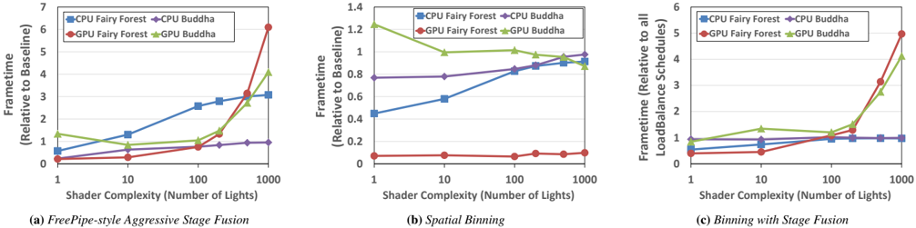
### Visual Description
## Charts/Graphs: Frametime Performance Across Different Rendering Techniques and Hardware
### Overview
This image presents three line charts, labeled (a), (b), and (c), each illustrating the "Frametime" performance relative to a baseline or other schedules, as "Shader Complexity (Number of Lights)" increases. The charts compare the performance of "CPU Fairy Forest", "CPU Buddha", "GPU Fairy Forest", and "GPU Buddha" across three different rendering techniques: "FreePipe-style Aggressive Stage Fusion", "Spatial Binning", and "Binning with Stage Fusion". The x-axis for all charts is logarithmic, representing shader complexity, while the y-axis is linear, representing frametime.
### Components/Axes
The image consists of three distinct sub-charts arranged horizontally. Each sub-chart shares a common x-axis label and legend, but has a unique y-axis label and scale.
**Common X-axis:**
- **Title:** "Shader Complexity (Number of Lights)"
- **Scale:** Logarithmic, ranging from 1 to 1000.
- **Markers:** 1, 10, 100, 1000.
**Common Legend (positioned in the top-right corner of each sub-chart):**
- **CPU Fairy Forest:** Blue square marker, blue line.
- **CPU Buddha:** Purple diamond marker, purple line.
- **GPU Fairy Forest:** Red circle marker, red line.
- **GPU Buddha:** Green triangle marker, green line.
**Chart (a) Specific Y-axis:**
- **Title:** "Frametime (Relative to Baseline)"
- **Scale:** Linear, ranging from 0 to 7.
- **Markers:** 0, 1, 2, 3, 4, 5, 6, 7.
**Chart (b) Specific Y-axis:**
- **Title:** "Frametime (Relative to Baseline)"
- **Scale:** Linear, ranging from 0 to 1.4.
- **Markers:** 0, 0.2, 0.4, 0.6, 0.8, 1.0, 1.2, 1.4.
**Chart (c) Specific Y-axis:**
- **Title:** "Frametime (Relative to all LoadBalance Schedules)"
- **Scale:** Linear, ranging from 0 to 6.
- **Markers:** 0, 1, 2, 3, 4, 5, 6.
### Detailed Analysis
#### (a) FreePipe-style Aggressive Stage Fusion
This chart, located in the bottom-left, shows frametime relative to baseline using "FreePipe-style Aggressive Stage Fusion".
- **CPU Fairy Forest (Blue Square):** The frametime starts at approximately 0.5 at 1 light, increases to about 1.3 at 10 lights, then to 2.6 at 100 lights, and finally reaches approximately 3.0 at 1000 lights. The trend is a steady increase, with a slight acceleration between 10 and 100 lights, then a slower increase.
- **CPU Buddha (Purple Diamond):** The frametime starts at approximately 0.3 at 1 light, increases to about 0.5 at 10 lights, then to 0.8 at 100 lights, and stabilizes around 0.9 at 1000 lights. The trend shows a moderate increase followed by a flattening.
- **GPU Fairy Forest (Red Circle):** The frametime starts very low, at approximately 0.2 at 1 light, remains low at about 0.3 at 10 lights, then increases to 0.8 at 100 lights, and sharply rises to approximately 5.5 at 1000 lights. The trend is relatively flat at low complexity, followed by a dramatic exponential increase at high complexity.
- **GPU Buddha (Green Triangle):** The frametime starts at approximately 1.3 at 1 light, decreases to about 0.9 at 10 lights, then increases to 1.5 at 100 lights, and sharply rises to approximately 3.8 at 1000 lights. The trend shows an initial decrease, followed by a sharp increase at higher complexities.
#### (b) Spatial Binning
This chart, located in the bottom-center, shows frametime relative to baseline using "Spatial Binning".
- **CPU Fairy Forest (Blue Square):** The frametime starts at approximately 0.45 at 1 light, increases to about 0.58 at 10 lights, then to 0.85 at 100 lights, and reaches approximately 0.95 at 1000 lights. The trend is a consistent, moderate increase.
- **CPU Buddha (Purple Diamond):** The frametime starts at approximately 0.78 at 1 light, remains around 0.78 at 10 lights, then increases slightly to 0.85 at 100 lights, and reaches approximately 0.95 at 1000 lights. The trend is largely flat at lower complexities, with a slight increase at higher complexities.
- **GPU Fairy Forest (Red Circle):** The frametime starts very low, at approximately 0.08 at 1 light, remains around 0.08 at 10 lights and 100 lights, and slightly increases to approximately 0.1 at 1000 lights. The trend is remarkably flat and consistently very low across all complexities.
- **GPU Buddha (Green Triangle):** The frametime starts at approximately 1.25 at 1 light, decreases to about 1.0 at 10 lights, remains around 1.0 at 100 lights, and slightly decreases to approximately 0.95 at 1000 lights. The trend shows an initial decrease, then flattens out.
#### (c) Binning with Stage Fusion
This chart, located in the bottom-right, shows frametime relative to all LoadBalance Schedules using "Binning with Stage Fusion".
- **CPU Fairy Forest (Blue Square):** The frametime starts at approximately 0.5 at 1 light, increases to about 0.6 at 10 lights, then to 0.7 at 100 lights, and remains around 0.7 at 1000 lights. The trend shows a slight increase followed by a flattening.
- **CPU Buddha (Purple Diamond):** The frametime starts at approximately 0.6 at 1 light, increases to about 0.7 at 10 lights, then to 0.8 at 100 lights, and remains around 0.8 at 1000 lights. The trend shows a slight increase followed by a flattening.
- **GPU Fairy Forest (Red Circle):** The frametime starts at approximately 0.4 at 1 light, increases to about 0.5 at 10 lights, then to 0.8 at 100 lights, and sharply rises to approximately 5.0 at 1000 lights. The trend is relatively flat at low complexity, followed by a dramatic exponential increase at high complexity.
- **GPU Buddha (Green Triangle):** The frametime starts at approximately 0.9 at 1 light, increases to about 1.2 at 10 lights, then to 1.5 at 100 lights, and sharply rises to approximately 4.0 at 1000 lights. The trend shows a steady increase at lower complexities, followed by a sharp exponential increase at high complexity.
### Key Observations
- **GPU Fairy Forest Performance:** In both "FreePipe-style Aggressive Stage Fusion" (a) and "Binning with Stage Fusion" (c), GPU Fairy Forest exhibits a dramatic increase in frametime at high shader complexities (1000 lights), becoming the worst performer. However, in "Spatial Binning" (b), GPU Fairy Forest consistently maintains the lowest frametime across all complexities.
- **CPU Performance Stability:** CPU-based methods (CPU Fairy Forest and CPU Buddha) generally show more stable and predictable frametime increases compared to GPU methods, especially at higher complexities, in charts (a) and (c). Their frametime curves tend to flatten or increase linearly rather than exponentially.
- **Spatial Binning Effectiveness:** "Spatial Binning" (b) appears to be highly effective for GPU Fairy Forest, keeping its frametime very low. It also shows that CPU Buddha and CPU Fairy Forest have frametimes below 1.0 (relative to baseline) for all complexities, suggesting good performance. GPU Buddha in (b) also performs well, staying below 1.25.
- **Impact of Stage Fusion:** The addition of "Stage Fusion" (a) and (c) seems to negatively impact GPU performance at high complexities, leading to significant frametime spikes for both GPU Fairy Forest and GPU Buddha.
- **CPU Buddha Consistency:** CPU Buddha generally maintains a relatively low and stable frametime across all three techniques and complexities, often performing better than CPU Fairy Forest, especially at higher complexities in (a) and (c).
### Interpretation
The data suggests that the choice of rendering technique significantly impacts performance, particularly for GPU-based rendering as shader complexity increases.
1. **Spatial Binning (b) is highly optimized for GPU Fairy Forest:** The "Spatial Binning" technique demonstrates exceptional efficiency for "GPU Fairy Forest", maintaining a frametime close to zero relative to the baseline, even with 1000 lights. This indicates that spatial binning effectively manages the workload for this specific GPU configuration and scene type, preventing the performance degradation seen in other techniques. CPU methods also perform well under spatial binning, staying below the baseline.
2. **Stage Fusion introduces scalability challenges for GPUs:** Both "FreePipe-style Aggressive Stage Fusion" (a) and "Binning with Stage Fusion" (c) show that when stage fusion is involved, GPU performance (especially "GPU Fairy Forest" and "GPU Buddha") degrades significantly and non-linearly at higher shader complexities. This suggests that the overhead or architectural limitations related to stage fusion become a bottleneck for GPUs when processing a large number of lights. The exponential rise in frametime indicates a potential resource exhaustion or a non-optimal scaling of the fusion process on GPUs.
3. **CPUs handle stage fusion complexity more gracefully:** In contrast to GPUs, CPU-based rendering ("CPU Fairy Forest" and "CPU Buddha") with stage fusion (a and c) shows a more controlled increase in frametime. While frametime does increase, it tends to flatten out or increase linearly, suggesting that CPUs might be better equipped to handle the specific type of workload introduced by stage fusion, or that their performance degradation model is different and less severe than GPUs in these scenarios. "CPU Buddha" consistently shows better or comparable performance to "CPU Fairy Forest" across all scenarios, indicating its potential efficiency.
4. **Baseline and Relative Performance:** The y-axis labels are crucial. In (a) and (b), "Relative to Baseline" implies a comparison to a standard or initial performance. In (c), "Relative to all LoadBalance Schedules" suggests a comparison against a set of load-balancing techniques, implying that the values represent how well "Binning with Stage Fusion" performs compared to other load-balancing approaches. Values below 1.0 are generally desirable, indicating better performance than the baseline/other schedules.
In summary, for scenarios with high shader complexity, "Spatial Binning" appears to be the superior technique, especially for GPU rendering. However, when "Stage Fusion" is employed, CPU-based rendering, particularly "CPU Buddha", demonstrates more robust and scalable performance compared to GPU-based methods, which suffer significant performance drops. This highlights a trade-off between different rendering techniques and hardware platforms depending on the specific demands of the scene (shader complexity) and the chosen optimization strategies.
</details>
Figure 5: Test scenes from our Reyes pipeline generated by Pikoc . The left scene, Bigguy, renders at 127.6 ms. The right scene, Teapot, renders at 85.1 ms.
<details>
<summary>Image 9 Details</summary>
### Visual Description
## 3D Renderings: Two Objects Displayed in Graphics Pipeline Windows
### Overview
The image displays two distinct 3D rendered objects, each presented within what appears to be a separate application window, against a solid black background. The objects are a stylized blue creature and a classic yellow teapot, both rendered with smooth shading. The right window's title bar explicitly identifies the application as "Mesa Pipeline".
### Components/Axes
The image is composed of two primary display regions, each representing a graphical output window:
1. **Left Display Region (Left Window)**:
* **Content**: A 3D model of a stylized, bipedal creature.
* **Background**: Solid black.
* **Window Frame**: A thin, light grey border is visible along the top and left edges, indicating a window boundary. The window title bar is present at the very top, but no text is clearly legible within it.
2. **Right Display Region (Right Window)**:
* **Content**: A 3D model of a teapot.
* **Background**: Solid black.
* **Window Frame**: A thin, light grey border is visible along the top and right edges, indicating a window boundary.
* **Window Title**: Located centrally within the top window frame, the text "Mesa Pipeline" is clearly legible.
### Detailed Analysis
**Left Display Region (Stylized Creature Model):**
* **Object Description**: The object is a 3D model of a creature, rendered in a uniform light blue color. It has a bulky, somewhat hunched posture.
* **Body Shape**: The torso is large and rounded, with visible folds or rolls suggesting a soft, fleshy form. The head is integrated into the upper torso, featuring what appear to be closed eyes or prominent brow ridges.
* **Limbs**: It possesses short, thick legs ending in broad, flat feet. The arms are also short and thick, with large, somewhat simplified hands.
* **Surface Properties**: The surface is smooth and matte, with subtle shading indicating curvature and depth. Highlights suggest a primary light source from the upper-left or front-left direction, casting soft shadows that define the contours of the body.
* **Positioning**: The creature is centered horizontally within its display region and occupies approximately 70-80% of the vertical space. It appears to be standing on an implied ground plane.
**Right Display Region (Teapot Model):**
* **Object Description**: The object is a 3D model of a teapot, rendered in a uniform light yellow color. This model is consistent with the "Utah Teapot," a standard reference object in computer graphics.
* **Body Shape**: The main body is spherical. It features a distinct lid with a small, rounded knob on top. A curved handle extends from the left side of the body, and a tapered spout extends from the right side.
* **Surface Properties**: Similar to the creature model, the teapot has a smooth, matte surface with subtle shading. Highlights and shadows indicate a primary light source from the upper-left or front-left, consistent with the lighting of the creature model.
* **Positioning**: The teapot is centered horizontally within its display region and occupies approximately 70-80% of the vertical space. It appears to be resting on an implied ground plane.
### Key Observations
* Both 3D models are rendered using a smooth shading technique (e.g., Gouraud or Phong shading), without visible textures or complex materials, suggesting a focus on geometric form and basic lighting.
* The lighting conditions appear consistent across both renderings, implying they might be generated by the same rendering engine or pipeline configuration.
* The black background provides a stark contrast, making the rendered objects stand out clearly.
* The presence of "Mesa Pipeline" in the title bar of the right window is a significant piece of information, indicating the software or graphics library used for rendering. Mesa is an open-source implementation of the OpenGL specification.
### Interpretation
The image serves as a demonstration of basic 3D rendering capabilities, likely showcasing the output of a graphics pipeline such as Mesa. The two distinct objects—a complex organic model (the creature) and a classic geometric primitive (the Utah Teapot)—illustrate the pipeline's ability to render different types of 3D geometry.
The consistent lighting and shading across both windows suggest that these are not merely static images but active renderings from a graphics application. The "Mesa Pipeline" label strongly implies that these are real-time or near real-time renders produced by the Mesa 3D Graphics Library, which is commonly used for software rendering or as an open-source driver for hardware acceleration. This type of output is typical for testing, development, or educational demonstrations of 3D graphics programming and rendering techniques. The simplicity of the rendering (smooth shading, no textures) points towards a focus on the underlying geometry processing and lighting calculations rather than advanced material properties or photorealism.
</details>
we achieved 9.44 million patches per second (Mp/s), vs. Micropolis's 12.92 Mp/s; while a direct comparison of GPUs is difficult, Micropolis ran on an AMD GPU with 1.13x more peak compute and 1.11x more peak bandwidth than ours. Our implementation is 1.37x slower, but Micropolis is a complex, heavily-optimized and -tuned implementation targeted to a single GPU, whereas ours is considerably simpler, easier to write, understand, and modify, and more portable. For many scenarios, these concerns may outweigh modest performance differences.
## 8 Conclusion
Programmable graphics pipelines offer a new opportunity for existing and novel rendering ideas to impact next-generation interactive graphics. Our contribution, the Piko framework, targets high performance with programmability. Piko's main design decisions are the use of binning to exploit spatial locality as a fundamental building block for programmable pipelines, and the decomposition of pipeline stages into AssignBin , Schedule and Process phases to enable high-level exploration of the optimization alternatives. This helps implement performance optimizations and enhance programmability and portability. More broadly, we hope our work contributes to the conversation about how to think about implementing programmable pipelines.
One of the most important challenges in this work is how a high-level programming system can enable the important optimizations nec- essary to generate efficient pipelines. We believe that emphasizing spatial locality, so prevalent in both hardware-accelerated graphics and in the fastest programmable pipelines, is a crucial ingredient in efficient implementations. In the near future, we hope to investigate two extensions to this work, non-uniform bin sizes (which may offer better load balance) and spatial binning in higher dimensions (for applications like voxel rendering and volume rendering). Certainly special-purpose hardware takes advantage of binning in the form of hierarchical or tiled rasterizers, low-precision on-chip depth buffers, texture derivative computation, among others. However, our current binning implementations are all in software. Could future GPU programming models offer more native support for programmable spatial locality and bins?
From the point of view of programmable graphics, Larrabee [Seiler et al. 2008] took a novel approach: it eschewed special-purpose hardware in favor of pipelines that were programmed at their core in software. One of the most interesting aspects of Larrabee's approach to graphics was software scheduling. Previous generations of GPUs had relied on hardware schedulers to distribute work to parallel units; the Larrabee architects instead advocated software control of scheduling. Piko's schedules are largely statically compilergenerated, avoiding the complex implementations of recent work on GPU-based software schedulers, but dynamic, efficient scheduling has clear advantages for dynamic workloads (the reason we leverage the GPU's scheduling hardware for limited distribution within Piko already). Exploring the benefits and drawbacks of more general dynamic work scheduling, such as more task-parallel strategies, is another interesting area of future work.
In this paper, we consider pipelines that are entirely implemented in software, as our underlying APIs have no direct access to fixedfunction units. As these APIs add this functionality (and this API design alone is itself an interesting research problem), certainly this is worth revisiting, for fixed-function units have significant advantages. A decade ago, hardware designers motivated fixed-function units (and fixed-function pipelines) with their large computational performance per area; today, they cite their superior power efficiency. Application programmers have also demonstrated remarkable success at folding, spindling, and mutilating existing pipelines to achieve complex effects for which those pipelines were never designed. It is certainly fair to say that fixed-function power efficiency and programmer creativity are possible reasons why programmable pipelines may never replace conventional approaches. But thinking about pipelines from a software perspective offers us the opportunity to explore a space of alternative rendering pipelines, possibly as prototypes for future hardware, that would not be considered in a hardware-focused environment. And it is vital to perform a fair comparison against the most capable and optimized programmable pipelines, ones that take advantage of load-balanced parallelism and data locality, to strike the right balance between hardware and software. We hope our work is a step in this direction.
## References
- AILA, T., AND LAINE, S. 2009. Understanding the efficiency of ray traversal on GPUs. In Proceedings of High Performance Graphics 2009 , 145-149.
- AILA, T., MIETTINEN, V., AND NORDLUND, P. 2003. Delay streams for graphics hardware. ACM Transactions on Graphics 22 , 3 (July), 792-800.
- ANDERSSON, J. 2009. Parallel graphics in Frostbite-current & future. In Beyond Programmable Shading (ACM SIGGRAPH 2009 Course) , ACM, New York, NY, USA, SIGGRAPH '09, 7:1-7:312.
- APODACA, A. A., AND MANTLE, M. W. 1990. RenderMan: Pursuing the future of graphics. IEEE Computer Graphics & Applications 10 , 4 (July), 44-49.
- COOK, R. L., CARPENTER, L., AND CATMULL, E. 1987. The Reyes image rendering architecture. In Computer Graphics (Proceedings of SIGGRAPH 87) , 95-102.
- ELDRIDGE, M., IGEHY, H., AND HANRAHAN, P. 2000. Pomegranate: A fully scalable graphics architecture. In Proceedings of ACM SIGGRAPH 2000 , Computer Graphics Proceedings, Annual Conference Series, 443-454.
- FATAHALIAN, K., HORN, D. R., KNIGHT, T. J., LEEM, L., HOUSTON, M., PARK, J. Y., EREZ, M., REN, M., AIKEN, A., DALLY, W. J., AND HANRAHAN, P. 2006. Sequoia: Programming the memory hierarchy. In SC '06: Proceedings of the 2006 ACM/IEEE Conference on Supercomputing , 83.
- FOLEY, T., AND HANRAHAN, P. 2011. Spark: modular, composable shaders for graphics hardware. ACM Transactions on Graphics 30 , 4 (July), 107:1-107:12.
- FUCHS, H., POULTON, J., EYLES, J., GREER, T., GOLDFEATHER, J., ELLSWORTH, D., MOLNAR, S., TURK, G., TEBBS, B., AND ISRAEL, L. 1989. Pixel-Planes 5: A heterogeneous multiprocessor graphics system using processor-enhanced memories. In Computer Graphics (Proceedings of SIGGRAPH 89) , vol. 23, 79-88.
- GUPTA, K., STUART, J., AND OWENS, J. D. 2012. A study of persistent threads style GPU programming for GPGPU workloads. In Proceedings of Innovative Parallel Computing , InPar '12.
- HASSELGREN, J., AND AKENINE-MÖLLER, T. 2007. PCU: The programmable culling unit. ACM Transactions on Graphics 26 , 3 (July), 92:1-92:10.
- HUMPHREYS, G., HOUSTON, M., NG, R., FRANK, R., AHERN, S., KIRCHNER, P., AND KLOSOWSKI, J. 2002. Chromium: A stream-processing framework for interactive rendering on clusters. ACM Transactions on Graphics 21 , 3 (July), 693-702.
- IMAGINATION TECHNOLOGIES LTD. 2011. POWERVR Series5 Graphics SGX architecture guide for developers , 5 July. Version 1.0.8.
- LAINE, S., AND KARRAS, T. 2011. High-performance software rasterization on GPUs. In High Performance Graphics , 79-88.
- LATTNER, C., AND ADVE, V. 2004. LLVM: A compilation framework for lifelong program analysis & transformation. In Proceedings of the 2004 International Symposium on Code Generation and Optimization , CGO '04, 75-86.
- LIU, F., HUANG, M.-C., LIU, X.-H., AND WU, E.-H. 2010. FreePipe: a programmable parallel rendering architecture for efficient multi-fragment effects. In I3D '10: Proceedings of the 2010 ACM SIGGRAPH Symposium on Interactive 3D Graphics and Games , 75-82.
- MARK, W. R., GLANVILLE, R. S., AKELEY, K., AND KILGARD, M. J. 2003. Cg: A system for programming graphics hardware in a C-like language. ACM Transactions on Graphics 22 , 3 (July), 896-907.
- MONTRYM, J. S., BAUM, D. R., DIGNAM, D. L., AND MIGDAL, C. J. 1997. InfiniteReality: A real-time graphics system. In Proceedings of SIGGRAPH 97 , Computer Graphics Proceedings, Annual Conference Series, 293-302.
- OLANO, M., AND LASTRA, A. 1998. A shading language on graphics hardware: The PixelFlow shading system. In Proceedings of SIGGRAPH 98 , Computer Graphics Proceedings, Annual Conference Series, 159-168.
- OLSON, T. J. 2012. Saving the planet, one handset at a time: Designing low-power, low-bandwidth GPUs. In ACM SIGGRAPH 2012 Mobile .
- PANTALEONI, J. 2011. VoxelPipe: A programmable pipeline for 3D voxelization. In High Performance Graphics , HPG '11, 99-106.
- PARKER, S. G., BIGLER, J., DIETRICH, A., FRIEDRICH, H., HOBEROCK, J., LUEBKE, D., MCALLISTER, D., MCGUIRE, M., MORLEY, K., ROBISON, A., AND STICH, M. 2010. OptiX: A general purpose ray tracing engine. ACM Transactions on Graphics 29 , 4 (July), 66:1-66:13.
- PATNEY, A., AND OWENS, J. D. 2008. Real-time Reyes-style adaptive surface subdivision. ACM Transactions on Graphics 27 , 5 (Dec.), 143:1-143:8.
- PEERCY, M. S., OLANO, M., AIREY, J., AND UNGAR, P. J. 2000. Interactive multi-pass programmable shading. In Proceedings of ACM SIGGRAPH 2000 , Computer Graphics Proceedings, Annual Conference Series, 425-432.
- POTMESIL, M., AND HOFFERT, E. M. 1989. The Pixel Machine: A parallel image computer. In Computer Graphics (Proceedings of SIGGRAPH 89) , vol. 23, 69-78.
- PURCELL, T. 2010. Fast tessellated rendering on Fermi GF100. In High Performance Graphics Hot3D .
- RAGAN-KELLEY, J., ADAMS, A., PARIS, S., LEVOY, M., AMARASINGHE, S., AND DURAND, F. 2012. Decoupling algorithms from schedules for easy optimization of image processing pipelines. ACM Transactions on Graphics 31 , 4 (July), 32:132:12.
- SANCHEZ, D., LO, D., YOO, R. M., SUGERMAN, J., AND KOZYRAKIS, C. 2011. Dynamic fine-grain scheduling of pipeline parallelism. In Proceedings of the 2011 International Conference on Parallel Architectures and Compilation Techniques , IEEE Computer Society, Washington, DC, USA, PACT '11, 22-32.
- SEILER, L., CARMEAN, D., SPRANGLE, E., FORSYTH, T., ABRASH, M., DUBEY, P., JUNKINS, S., LAKE, A., SUGERMAN, J., CAVIN, R., ESPASA, R., GROCHOWSKI, E., JUAN, T., AND HANRAHAN, P. 2008. Larrabee: A many-core x86 architecture for visual computing. ACM Transactions on Graphics 27 , 3 (Aug.), 18:1-18:15.
- STOLL, G., ELDRIDGE, M., PATTERSON, D., WEBB, A., BERMAN, S., LEVY, R., CAYWOOD, C., TAVEIRA, M., HUNT, S., AND HANRAHAN, P. 2001. Lightning-2: A high-performance
display subsystem for PC clusters. In Proceedings of ACM SIGGRAPH 2001 , Computer Graphics Proceedings, Annual Conference Series, 141-148.
- SUGERMAN, J., FATAHALIAN, K., BOULOS, S., AKELEY, K., AND HANRAHAN, P. 2009. GRAMPS: A programming model for graphics pipelines. ACM Transactions on Graphics 28 , 1 (Jan.), 4:1-4:11.
- THIES, W., KARCZMAREK, M., AND AMARASINGHE, S. P. 2002. StreamIt: A language for streaming applications. In Proceedings of the 11th International Conference on Compiler Construction , R. N. Horspool, Ed., Lecture Notes in Computer Science. Springer-Verlag, Apr., 179-196.
- TZENG, S., PATNEY, A., AND OWENS, J. D. 2010. Task management for irregular-parallel workloads on the GPU. In Proceedings of High Performance Graphics 2010 , 29-37.
- WEBER, T., WIMMER, M., AND OWENS, J. D. 2015. Parallel Reyes-style adaptive subdivision with bounded memory usage. In Proceedings of the ACM SIGGRAPH Symposium on Interactive 3D Graphics and Games , i3D 2015.
- ZHOU, K., HOU, Q., REN, Z., GONG, M., SUN, X., AND GUO, B. 2009. RenderAnts: Interactive Reyes rendering on GPUs. ACM Transactions on Graphics 28 , 5 (Dec.), 155:1-155:11.