1410.5401v2

## Neural Turing Machines Alex Graves Greg Wayne Ivo Danihelka gravesa@google.com gregwayne@google.com danihelka@google.com Google DeepMind, London, UK ## Abstract We extend the capabilities of neural networks by coupling them to external memory resources, which they can interact with by attentional processes. The combined system is analogous to a Turing Machine or Von Neumann architecture but is differentiable end-toend, allowing it to be efficiently trained with gradient descent. Preliminary results demonstrate that Neural Turing Machines can infer simple algorithms such as copying, sorting, and associative recall from input and output examples. ## 1 Introduction Computer programs make use of three fundamental mechanisms: elementary operations (e.g., arithmetic operations), logical flow control (branching), and external memory, which can be written to and read from in the course of computation (Von Neumann, 1945). Despite its wide-ranging success in modelling complicated data, modern machine learning has largely neglected the use of logical flow control and external memory. Recurrent neural networks (RNNs) stand out from other machine learning methods for their ability to learn and carry out complicated transformations of data over extended periods of time. Moreover, it is known that RNNs are Turing-Complete (Siegelmann and Sontag, 1995), and therefore have the capacity to simulate arbitrary procedures, if properly wired. Yet what is possible in principle is not always what is simple in practice. We therefore enrich the capabilities of standard recurrent networks to simplify the solution of algorithmic tasks. This enrichment is primarily via a large, addressable memory, so, by analogy to Turing's enrichment of finite-state machines by an infinite memory tape, we dub our device a 'Neural Turing Machine' (NTM). Unlike a Turing machine, an NTM is a differentiable computer that can be trained by gradient descent, yielding a practical mechanism for learning programs. In human cognition, the process that shares the most similarity to algorithmic operation is known as 'working memory.' While the mechanisms of working memory remain somewhat obscure at the level of neurophysiology, the verbal definition is understood to mean a capacity for short-term storage of information and its rule-based manipulation (Baddeley et al., 2009). In computational terms, these rules are simple programs, and the stored information constitutes the arguments of these programs. Therefore, an NTM resembles a working memory system, as it is designed to solve tasks that require the application of approximate rules to 'rapidly-created variables.' Rapidly-created variables (Hadley, 2009) are data that are quickly bound to memory slots, in the same way that the number 3 and the number 4 are put inside registers in a conventional computer and added to make 7 (Minsky, 1967). An NTM bears another close resemblance to models of working memory since the NTMarchitecture uses an attentional process to read from and write to memory selectively. In contrast to most models of working memory, our architecture can learn to use its working memory instead of deploying a fixed set of procedures over symbolic data. The organisation of this report begins with a brief review of germane research on working memory in psychology, linguistics, and neuroscience, along with related research in artificial intelligence and neural networks. We then describe our basic contribution, a memory architecture and attentional controller that we believe is well-suited to the performance of tasks that require the induction and execution of simple programs. To test this architecture, we have constructed a battery of problems, and we present their precise descriptions along with our results. We conclude by summarising the strengths of the architecture. ## 2 Foundational Research ## 2.1 Psychology and Neuroscience The concept of working memory has been most heavily developed in psychology to explain the performance of tasks involving the short-term manipulation of information. The broad picture is that a 'central executive' focuses attention and performs operations on data in a memory buffer (Baddeley et al., 2009). Psychologists have extensively studied the capacity limitations of working memory, which is often quantified by the number of 'chunks' of information that can be readily recalled (Miller, 1956). 1 These capacity limitations lead toward an understanding of structural constraints in the human working memory system, but in our own work we are happy to exceed them. In neuroscience, the working memory process has been ascribed to the functioning of a system composed of the prefrontal cortex and basal ganglia (Goldman-Rakic, 1995). Typ- 1 There remains vigorous debate about how best to characterise capacity limitations (Barrouillet et al., 2004). ical experiments involve recording from a single neuron or group of neurons in prefrontal cortex while a monkey is performing a task that involves observing a transient cue, waiting through a 'delay period,' then responding in a manner dependent on the cue. Certain tasks elicit persistent firing from individual neurons during the delay period or more complicated neural dynamics. A recent study quantified delay period activity in prefrontal cortex for a complex, context-dependent task based on measures of 'dimensionality' of the population code and showed that it predicted memory performance (Rigotti et al., 2013). Modeling studies of working memory range from those that consider how biophysical circuits could implement persistent neuronal firing (Wang, 1999) to those that try to solve explicit tasks (Hazy et al., 2006) (Dayan, 2008) (Eliasmith, 2013). Of these, Hazy et al.'s model is the most relevant to our work, as it is itself analogous to the Long Short-Term Memory architecture, which we have modified ourselves. As in our architecture, Hazy et al.'s has mechanisms to gate information into memory slots, which they use to solve a memory task constructed of nested rules. In contrast to our work, the authors include no sophisticated notion of memory addressing, which limits the system to storage and recall of relatively simple, atomic data. Addressing, fundamental to our work, is usually left out from computational models in neuroscience, though it deserves to be mentioned that Gallistel and King (Gallistel and King, 2009) and Marcus (Marcus, 2003) have argued that addressing must be implicated in the operation of the brain. ## 2.2 Cognitive Science and Linguistics Historically, cognitive science and linguistics emerged as fields at roughly the same time as artificial intelligence, all deeply influenced by the advent of the computer (Chomsky, 1956) (Miller, 2003). Their intentions were to explain human mental behaviour based on information or symbol-processing metaphors. In the early 1980s, both fields considered recursive or procedural (rule-based) symbol-processing to be the highest mark of cognition. The Parallel Distributed Processing (PDP) or connectionist revolution cast aside the symbol-processing metaphor in favour of a so-called 'sub-symbolic' description of thought processes (Rumelhart et al., 1986). Fodor and Pylyshyn (Fodor and Pylyshyn, 1988) famously made two barbed claims about the limitations of neural networks for cognitive modeling. They first objected that connectionist theories were incapable of variable-binding , or the assignment of a particular datum to a particular slot in a data structure. In language, variable-binding is ubiquitous; for example, when one produces or interprets a sentence of the form, 'Mary spoke to John,' one has assigned 'Mary' the role of subject, 'John' the role of object, and 'spoke to' the role of the transitive verb. Fodor and Pylyshyn also argued that neural networks with fixedlength input domains could not reproduce human capabilities in tasks that involve processing variable-length structures . In response to this criticism, neural network researchers including Hinton (Hinton, 1986), Smolensky (Smolensky, 1990), Touretzky (Touretzky, 1990), Pollack (Pollack, 1990), Plate (Plate, 2003), and Kanerva (Kanerva, 2009) investigated specific mechanisms that could support both variable-binding and variable-length structure within a connectionist framework. Our architecture draws on and potentiates this work. Recursive processing of variable-length structures continues to be regarded as a hallmark of human cognition. In the last decade, a firefight in the linguistics community staked several leaders of the field against one another. At issue was whether recursive processing is the 'uniquely human' evolutionary innovation that enables language and is specialized to language, a view supported by Fitch, Hauser, and Chomsky (Fitch et al., 2005), or whether multiple new adaptations are responsible for human language evolution and recursive processing predates language (Jackendoff and Pinker, 2005). Regardless of recursive processing's evolutionary origins, all agreed that it is essential to human cognitive flexibility. ## 2.3 Recurrent Neural Networks Recurrent neural networks constitute a broad class of machines with dynamic state; that is, they have state whose evolution depends both on the input to the system and on the current state. In comparison to hidden Markov models, which also contain dynamic state, RNNs have a distributed state and therefore have significantly larger and richer memory and computational capacity. Dynamic state is crucial because it affords the possibility of context-dependent computation; a signal entering at a given moment can alter the behaviour of the network at a much later moment. A crucial innovation to recurrent networks was the Long Short-Term Memory (LSTM) (Hochreiter and Schmidhuber, 1997). This very general architecture was developed for a specific purpose, to address the 'vanishing and exploding gradient' problem (Hochreiter et al., 2001a), which we might relabel the problem of 'vanishing and exploding sensitivity.' LSTM ameliorates the problem by embedding perfect integrators (Seung, 1998) for memory storage in the network. The simplest example of a perfect integrator is the equation x ( t + 1) = x ( t ) + i ( t ) , where i ( t ) is an input to the system. The implicit identity matrix I x ( t ) means that signals do not dynamically vanish or explode. If we attach a mechanism to this integrator that allows an enclosing network to choose when the integrator listens to inputs, namely, a programmable gate depending on context, we have an equation of the form x ( t + 1) = x ( t ) + g ( context ) i ( t ) . We can now selectively store information for an indefinite length of time. Recurrent networks readily process variable-length structures without modification. In sequential problems, inputs to the network arrive at different times, allowing variablelength or composite structures to be processed over multiple steps. Because they natively handle variable-length structures, they have recently been used in a variety of cognitive problems, including speech recognition (Graves et al., 2013; Graves and Jaitly, 2014), text generation (Sutskever et al., 2011), handwriting generation (Graves, 2013) and machine translation (Sutskever et al., 2014). Considering this property, we do not feel that it is urgent or even necessarily valuable to build explicit parse trees to merge composite structures greedily (Pollack, 1990) (Socher et al., 2012) (Frasconi et al., 1998). 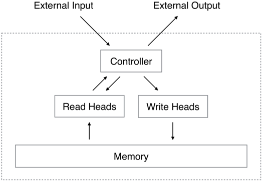Other important precursors to our work include differentiable models of attention (Graves, Figure 1: Neural Turing Machine Architecture. During each update cycle, the controller network receives inputs from an external environment and emits outputs in response. It also reads to and writes from a memory matrix via a set of parallel read and write heads. The dashed line indicates the division between the NTM circuit and the outside world. <details> <summary>Image 1 Details</summary>  ### Visual Description ## Block Diagram: System Architecture Overview ### Overview The diagram illustrates a simplified system architecture with data flow between components. It depicts bidirectional communication between a central controller and peripheral systems, with external input/output interfaces and memory storage. ### Components/Axes 1. **External Input** (Top-left): Arrows point toward the controller, indicating data entry point. 2. **Controller** (Central): Rectangular box acting as the central processing unit. 3. **Read Heads** (Bottom-left): Connected to memory via upward arrow, suggesting data retrieval. 4. **Write Heads** (Bottom-right): Connected to memory via downward arrow, indicating data storage. 5. **Memory** (Bottom): Horizontal rectangle serving as data storage medium. 6. **External Output** (Top-right): Arrows point away from controller, showing data exit point. ### Flow Relationships - External Input → Controller (unidirectional) - Controller ↔ Read Heads (bidirectional) - Controller ↔ Write Heads (bidirectional) - Read Heads → Memory (unidirectional) - Write Heads → Memory (unidirectional) - Controller → External Output (unidirectional) ### Key Observations 1. The controller acts as the central hub for all data processing. 2. Memory operates in a read/write architecture with dedicated interfaces. 3. External communication is strictly input/output with no direct memory access. 4. Bidirectional controller connections suggest real-time processing capabilities. ### Interpretation This architecture resembles a simplified computer memory controller system: - The controller manages data flow between external systems and internal memory - Read/Write Heads represent memory access interfaces - Bidirectional controller connections imply command/acknowledgment signaling - The design emphasizes separation of concerns between processing (controller) and storage (memory) The diagram suggests a Von Neumann architecture variant with explicit memory controller separation. The bidirectional controller connections indicate potential for complex command signaling beyond simple data transfer, possibly including error correction or timing synchronization protocols. </details> 2013) (Bahdanau et al., 2014) and program search (Hochreiter et al., 2001b) (Das et al., 1992), constructed with recurrent neural networks. ## 3 Neural Turing Machines A Neural Turing Machine (NTM) architecture contains two basic components: a neural network controller and a memory bank. Figure 1 presents a high-level diagram of the NTM architecture. Like most neural networks, the controller interacts with the external world via input and output vectors. Unlike a standard network, it also interacts with a memory matrix using selective read and write operations. By analogy to the Turing machine we refer to the network outputs that parametrise these operations as 'heads.' Crucially, every component of the architecture is differentiable, making it straightforward to train with gradient descent. We achieved this by defining 'blurry' read and write operations that interact to a greater or lesser degree with all the elements in memory (rather than addressing a single element, as in a normal Turing machine or digital computer). The degree of blurriness is determined by an attentional 'focus' mechanism that constrains each read and write operation to interact with a small portion of the memory, while ignoring the rest. Because interaction with the memory is highly sparse, the NTM is biased towards storing data without interference. The memory location brought into attentional focus is determined by specialised outputs emitted by the heads. These outputs define a normalised weighting over the rows in the memory matrix (referred to as memory 'locations'). Each weighting, one per read or write head, defines the degree to which the head reads or writes at each location. A head can thereby attend sharply to the memory at a single location or weakly to the memory at many locations. ## 3.1 Reading Let M t be the contents of the N × M memory matrix at time t, where N is the number of memory locations, and M is the vector size at each location. Let w t be a vector of weightings over the N locations emitted by a read head at time t . Since all weightings are normalised, the N elements w t ( i ) of w t obey the following constraints: <!-- formula-not-decoded --> The length M read vector r t returned by the head is defined as a convex combination of the row-vectors M t ( i ) in memory: <!-- formula-not-decoded --> which is clearly differentiable with respect to both the memory and the weighting. ## 3.2 Writing Taking inspiration from the input and forget gates in LSTM, we decompose each write into two parts: an erase followed by an add . Given a weighting w t emitted by a write head at time t , along with an erase vector e t whose M elements all lie in the range (0 , 1) , the memory vectors M t -1 ( i ) from the previous time-step are modified as follows: <!-- formula-not-decoded --> where 1 is a row-vector of all 1 -s, and the multiplication against the memory location acts point-wise. Therefore, the elements of a memory location are reset to zero only if both the weighting at the location and the erase element are one; if either the weighting or the erase is zero, the memory is left unchanged. When multiple write heads are present, the erasures can be performed in any order, as multiplication is commutative. Each write head also produces a length M add vector a t , which is added to the memory after the erase step has been performed: <!-- formula-not-decoded --> Once again, the order in which the adds are performed by multiple heads is irrelevant. The combined erase and add operations of all the write heads produces the final content of the memory at time t . Since both erase and add are differentiable, the composite write operation is differentiable too. Note that both the erase and add vectors have M independent components, allowing fine-grained control over which elements in each memory location are modified. 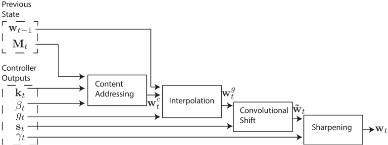Figure 2: Flow Diagram of the Addressing Mechanism. The key vector , k t , and key strength , β t , are used to perform content-based addressing of the memory matrix, M t . The resulting content-based weighting is interpolated with the weighting from the previous time step based on the value of the interpolation gate , g t . The shift weighting , s t , determines whether and by how much the weighting is rotated. Finally, depending on γ t , the weighting is sharpened and used for memory access. <details> <summary>Image 2 Details</summary>  ### Visual Description ## Block Diagram: Control System Processing Pipeline ### Overview The diagram illustrates a sequential data processing pipeline for a control system. It begins with inputs from a "Previous State" and "Controller Outputs," which are processed through five stages: Content Addressing, Interpolation, Convolutional Shift, and Sharpening. The final output is labeled **w_t**, representing the processed state at time **t**. --- ### Components/Axes 1. **Previous State** - Contains two variables: - **w_t-1**: Previous weight vector (input to Content Addressing). - **M_t**: Matrix associated with the previous state (input to Content Addressing). 2. **Controller Outputs** - Five variables feeding into Content Addressing: - **k_t**: Gain parameter. - **β_t**: Beta parameter. - **g_t**: Gamma parameter. - **s_t**: Sigma parameter. - **γ_t**: Additional control signal. 3. **Content Addressing** - Inputs: **w_t-1**, **M_t**, **k_t**, **β_t**, **g_t**, **s_t**, **γ_t**. - Output: **w_c** (content-addressed vector). 4. **Interpolation** - Input: **w_c**. - Output: **w_g** (interpolated vector). 5. **Convolutional Shift** - Input: **w_g**. - Output: **w_t~** (convolutionally shifted vector). 6. **Sharpening** - Input: **w_t~**. - Output: **w_t** (final processed state). --- ### Flow and Relationships - **Data Flow**: 1. **Previous State** and **Controller Outputs** are combined as inputs to **Content Addressing**. 2. **Content Addressing** processes these inputs to produce **w_c**, which is passed to **Interpolation**. 3. **Interpolation** generates **w_g**, which is fed into **Convolutional Shift**. 4. **Convolutional Shift** outputs **w_t~**, which is refined by **Sharpening** to produce **w_t**. - **Temporal Dependency**: The use of **w_t-1** (previous state) suggests the system incorporates historical data for decision-making. --- ### Key Observations 1. **Modular Design**: Each block performs a distinct transformation (e.g., interpolation, convolutional operations). 2. **Controller Integration**: Controller outputs (**k_t**, **β_t**, etc.) directly influence the Content Addressing stage, enabling real-time adjustments. 3. **Temporal Context**: The system retains memory of the previous state (**w_t-1**, **M_t**) to inform current processing. 4. **Final Output**: **w_t** represents the culmination of all transformations, likely used for system control or feedback. --- ### Interpretation This pipeline appears to model a **reinforcement learning** or **adaptive control system** where: - **Content Addressing** selects relevant features from historical data (**w_t-1**, **M_t**) and controller signals. - **Interpolation** and **Convolutional Shift** refine these features spatially or temporally. - **Sharpening** enhances critical details in the output (**w_t**), possibly for decision-making or actuation. The system’s reliance on **w_t-1** and **M_t** implies it operates in a dynamic environment requiring memory of past states. The inclusion of multiple controller parameters (**k_t**, **β_t**, etc.) suggests fine-grained tunability for optimization or stability. No numerical data or trends are present in the diagram; it focuses on architectural relationships and data flow. </details> ## 3.3 Addressing Mechanisms Although we have now shown the equations of reading and writing, we have not described how the weightings are produced. These weightings arise by combining two addressing mechanisms with complementary facilities. The first mechanism, 'content-based addressing,' focuses attention on locations based on the similarity between their current values and values emitted by the controller. This is related to the content-addressing of Hopfield networks (Hopfield, 1982). The advantage of content-based addressing is that retrieval is simple, merely requiring the controller to produce an approximation to a part of the stored data, which is then compared to memory to yield the exact stored value. However, not all problems are well-suited to content-based addressing. In certain tasks the content of a variable is arbitrary, but the variable still needs a recognisable name or address. Arithmetic problems fall into this category: the variable x and the variable y can take on any two values, but the procedure f ( x, y ) = x × y should still be defined. A controller for this task could take the values of the variables x and y , store them in different addresses, then retrieve them and perform a multiplication algorithm. In this case, the variables are addressed by location, not by content. We call this form of addressing 'location-based addressing.' Content-based addressing is strictly more general than location-based addressing as the content of a memory location could include location information inside it. In our experiments however, providing location-based addressing as a primitive operation proved essential for some forms of generalisation, so we employ both mechanisms concurrently. Figure 2 presents a flow diagram of the entire addressing system that shows the order of operations for constructing a weighting vector when reading or writing. ## 3.3.1 Focusing by Content For content-addressing, each head (whether employed for reading or writing) first produces a length M key vector k t that is compared to each vector M t ( i ) by a similarity measure K [ · , · ] . The content-based system produces a normalised weighting w c t based on the similarity and a positive key strength , β t , which can amplify or attenuate the precision of the focus: <!-- formula-not-decoded --> In our current implementation, the similarity measure is cosine similarity: <!-- formula-not-decoded --> ## 3.3.2 Focusing by Location The location-based addressing mechanism is designed to facilitate both simple iteration across the locations of the memory and random-access jumps. It does so by implementing a rotational shift of a weighting. For example, if the current weighting focuses entirely on a single location, a rotation of 1 would shift the focus to the next location. A negative shift would move the weighting in the opposite direction. Prior to rotation, each head emits a scalar interpolation gate g t in the range (0 , 1) . The value of g is used to blend between the weighting w t -1 produced by the head at the previous time-step and the weighting w c t produced by the content system at the current time-step, yielding the gated weighting w g t : <!-- formula-not-decoded --> If the gate is zero, then the content weighting is entirely ignored, and the weighting from the previous time step is used. Conversely, if the gate is one, the weighting from the previous iteration is ignored, and the system applies content-based addressing. After interpolation, each head emits a shift weighting s t that defines a normalised distribution over the allowed integer shifts. For example, if shifts between -1 and 1 are allowed, s t has three elements corresponding to the degree to which shifts of -1, 0 and 1 are performed. The simplest way to define the shift weightings is to use a softmax layer of the appropriate size attached to the controller. We also experimented with another technique, where the controller emits a single scalar that is interpreted as the lower bound of a width one uniform distribution over shifts. For example, if the shift scalar is 6.7, then s t (6) = 0 . 3 , s t (7) = 0 . 7 , and the rest of s t is zero. If we index the N memory locations from 0 to N -1 , the rotation applied to w g t by s t can be expressed as the following circular convolution: <!-- formula-not-decoded --> where all index arithmetic is computed modulo N . The convolution operation in Equation (8) can cause leakage or dispersion of weightings over time if the shift weighting is not sharp. For example, if shifts of -1, 0 and 1 are given weights of 0.1, 0.8 and 0.1, the rotation will transform a weighting focused at a single point into one slightly blurred over three points. To combat this, each head emits one further scalar γ t ≥ 1 whose effect is to sharpen the final weighting as follows: <!-- formula-not-decoded --> The combined addressing system of weighting interpolation and content and locationbased addressing can operate in three complementary modes. One, a weighting can be chosen by the content system without any modification by the location system. Two, a weighting produced by the content addressing system can be chosen and then shifted. This allows the focus to jump to a location next to, but not on, an address accessed by content; in computational terms this allows a head to find a contiguous block of data, then access a particular element within that block. Three, a weighting from the previous time step can be rotated without any input from the content-based addressing system. This allows the weighting to iterate through a sequence of addresses by advancing the same distance at each time-step. ## 3.4 Controller Network The NTM architecture architecture described above has several free parameters, including the size of the memory, the number of read and write heads, and the range of allowed location shifts. But perhaps the most significant architectural choice is the type of neural network used as the controller. In particular, one has to decide whether to use a recurrent or feedforward network. A recurrent controller such as LSTM has its own internal memory that can complement the larger memory in the matrix. If one compares the controller to the central processing unit in a digital computer (albeit with adaptive rather than predefined instructions) and the memory matrix to RAM, then the hidden activations of the recurrent controller are akin to the registers in the processor. They allow the controller to mix information across multiple time steps of operation. On the other hand a feedforward controller can mimic a recurrent network by reading and writing at the same location in memory at every step. Furthermore, feedforward controllers often confer greater transparency to the network's operation because the pattern of reading from and writing to the memory matrix is usually easier to interpret than the internal state of an RNN. However, one limitation of a feedforward controller is that the number of concurrent read and write heads imposes a bottleneck on the type of computation the NTM can perform. With a single read head, it can perform only a unary transform on a single memory vector at each time-step, with two read heads it can perform binary vector transforms, and so on. Recurrent controllers can internally store read vectors from previous time-steps, so do not suffer from this limitation. ## 4 Experiments This section presents preliminary experiments on a set of simple algorithmic tasks such as copying and sorting data sequences. The goal was not only to establish that NTM is able to solve the problems, but also that it is able to do so by learning compact internal programs. The hallmark of such solutions is that they generalise well beyond the range of the training data. For example, we were curious to see if a network that had been trained to copy sequences of length up to 20 could copy a sequence of length 100 with no further training. For all the experiments we compared three architectures: NTM with a feedforward controller, NTM with an LSTM controller, and a standard LSTM network. Because all the tasks were episodic, we reset the dynamic state of the networks at the start of each input sequence. For the LSTM networks, this meant setting the previous hidden state equal to a learned bias vector. For NTM the previous state of the controller, the value of the previous read vectors, and the contents of the memory were all reset to bias values. All the tasks were supervised learning problems with binary targets; all networks had logistic sigmoid output layers and were trained with the cross-entropy objective function. Sequence prediction errors are reported in bits-per-sequence. For more details about the experimental parameters see Section 4.6. ## 4.1 Copy The copy task tests whether NTM can store and recall a long sequence of arbitrary information. The network is presented with an input sequence of random binary vectors followed by a delimiter flag. Storage and access of information over long time periods has always been problematic for RNNs and other dynamic architectures. We were particularly interested to see if an NTM is able to bridge longer time delays than LSTM. The networks were trained to copy sequences of eight bit random vectors, where the sequence lengths were randomised between 1 and 20. The target sequence was simply a copy of the input sequence (without the delimiter flag). Note that no inputs were presented to the network while it receives the targets, to ensure that it recalls the entire sequence with no intermediate assistance. 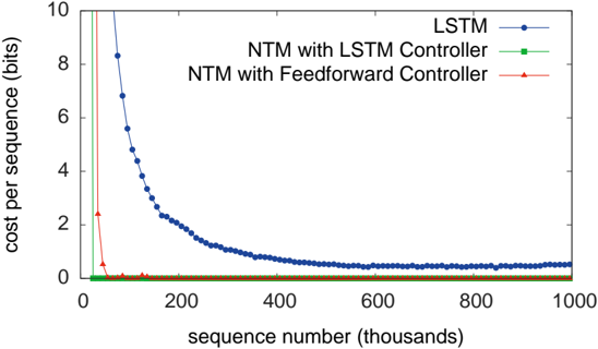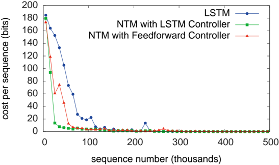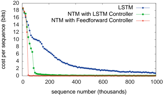As can be seen from Figure 3, NTM (with either a feedforward or LSTM controller) learned much faster than LSTM alone, and converged to a lower cost. The disparity between the NTM and LSTM learning curves is dramatic enough to suggest a qualitative, Figure 3: Copy Learning Curves. <details> <summary>Image 3 Details</summary>  ### Visual Description ## Line Graph: Cost per Sequence vs. Sequence Number (Thousands) ### Overview The image is a line graph comparing the cost per sequence (in bits) across three different models: LSTM, NTM with LSTM Controller, and NTM with Feedforward Controller. The x-axis represents sequence numbers (in thousands), and the y-axis represents cost per sequence (in bits). The graph shows distinct trends for each model, with the LSTM model exhibiting a sharp decline in cost, while the NTM controllers remain stable at near-zero cost. --- ### Components/Axes - **X-axis**: Labeled "sequence number (thousands)", ranging from 0 to 1000 (in thousands). - **Y-axis**: Labeled "cost per sequence (bits)", ranging from 0 to 10. - **Legend**: Located on the right side of the graph, with three entries: - **Blue line with circles**: LSTM - **Green line with squares**: NTM with LSTM Controller - **Red line with triangles**: NTM with Feedforward Controller --- ### Detailed Analysis 1. **LSTM (Blue Line)**: - Starts at approximately **8.5 bits** at sequence 0. - Declines sharply to **~0.5 bits** by sequence 200k. - Plateaus at **~0.5 bits** for sequences 200k–1000k. - Data points are plotted as circles. 2. **NTM with LSTM Controller (Green Line)**: - Remains at **0 bits** for all sequence numbers. - Data points are plotted as squares. 3. **NTM with Feedforward Controller (Red Line)**: - Remains at **0 bits** for all sequence numbers. - Data points are plotted as triangles. --- ### Key Observations - The LSTM model shows a **rapid decrease in cost** (from ~8.5 to ~0.5 bits) over the first 200k sequences, followed by stabilization. - Both NTM controllers (LSTM and Feedforward) maintain **zero cost** across all sequence numbers, indicating perfect efficiency or no cost incurred. - The LSTM model’s cost reduction suggests improved performance or optimization over time, while the NTM controllers are consistently optimal from the start. --- ### Interpretation - **LSTM Behavior**: The sharp decline in cost for the LSTM model implies that its performance improves as it processes more sequences, possibly due to learning or adaptive mechanisms. The plateau at ~0.5 bits suggests a lower bound on its efficiency. - **NTM Controllers**: The NTM with LSTM Controller and NTM with Feedforward Controller both achieve **zero cost**, indicating they are either inherently more efficient or designed to avoid cost entirely. This could reflect architectural advantages or task-specific optimizations. - **Comparison**: The LSTM model starts with higher costs but converges toward the NTM controllers’ efficiency over time. This highlights a trade-off between initial performance and long-term optimization. --- ### Spatial Grounding and Trend Verification - **Legend Placement**: Right-aligned, clearly associating colors with models. - **Line Trends**: - LSTM (blue): Steep downward slope followed by a flat line. - NTM Controllers (green/red): Horizontal lines at 0. - **Data Point Consistency**: All data points match their legend colors (blue circles for LSTM, green squares for NTM with LSTM Controller, red triangles for NTM with Feedforward Controller). --- ### Content Details - **LSTM Data Points**: - Sequence 0: ~8.5 bits - Sequence 200k: ~0.5 bits - Sequence 1000k: ~0.5 bits - **NTM Controllers**: All data points at 0 bits across all sequences. --- ### Final Notes The graph demonstrates that while LSTM models improve efficiency over time, NTM controllers with specialized architectures (LSTM or Feedforward) achieve optimal performance from the outset. This could inform decisions about model selection based on computational constraints and task requirements. </details> rather than quantitative, difference in the way the two models solve the problem. 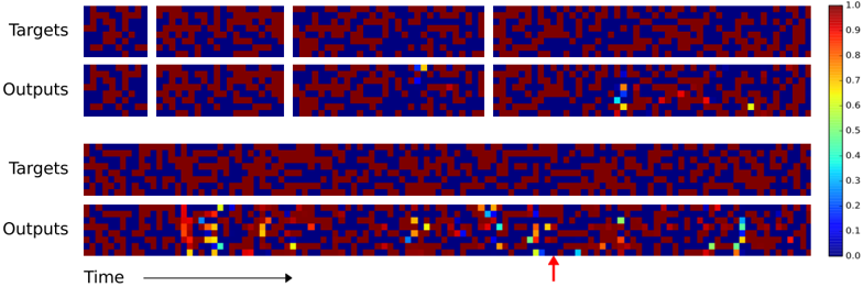We also studied the ability of the networks to generalise to longer sequences than seen during training (that they can generalise to novel vectors is clear from the training error). Figures 4 and 5 demonstrate that the behaviour of LSTM and NTM in this regime is radically different. NTM continues to copy as the length increases 2 , while LSTM rapidly degrades beyond length 20. The preceding analysis suggests that NTM, unlike LSTM, has learned some form of copy algorithm. To determine what this algorithm is, we examined the interaction between the controller and the memory (Figure 6). We believe that the sequence of operations performed by the network can be summarised by the following pseudocode: ``` ``` ## end while This is essentially how a human programmer would perform the same task in a low- 2 The limiting factor was the size of the memory (128 locations), after which the cyclical shifts wrapped around and previous writes were overwritten. 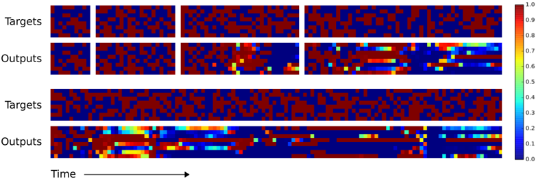Figure 4: NTM Generalisation on the Copy Task. The four pairs of plots in the top row depict network outputs and corresponding copy targets for test sequences of length 10, 20, 30, and 50, respectively. The plots in the bottom row are for a length 120 sequence. The network was only trained on sequences of up to length 20. The first four sequences are reproduced with high confidence and very few mistakes. The longest one has a few more local errors and one global error: at the point indicated by the red arrow at the bottom, a single vector is duplicated, pushing all subsequent vectors one step back. Despite being subjectively close to a correct copy, this leads to a high loss. <details> <summary>Image 4 Details</summary>  ### Visual Description ## Heatmap Visualization: Target vs. Output Patterns Over Time ### Overview The image presents a comparative visualization of "Targets" and "Outputs" across two distinct formats: a 2x2 grid of small panels (top section) and two elongated panels (bottom section). Both sections use a color-coded heatmap to represent values, with a vertical color scale from 0.0 (blue) to 1.0 (red). A red arrow highlights a specific region in the bottom "Outputs" panel. --- ### Components/Axes 1. **Top Section (2x2 Grid)**: - **Labels**: - Top row: "Targets" (left) and "Outputs" (right). - Bottom row: Repeats "Targets" and "Outputs". - **Structure**: - Four equal-sized panels arranged in a 2x2 grid. - No explicit axes or numerical labels. - **Color Scale**: - Vertical legend on the right (0.0–1.0), with red (1.0) at the top and blue (0.0) at the bottom. 2. **Bottom Section (Long Panels)**: - **Labels**: - Top row: "Targets" (left) and "Outputs" (right). - Bottom row: Repeats "Targets" and "Outputs". - **Axes**: - Horizontal axis labeled "Time" with an arrow pointing right. - No explicit y-axis label. - **Color Scale**: - Same vertical legend as the top section. --- ### Detailed Analysis 1. **Top Section**: - **Targets Panels**: - Dominated by red (high values) and blue (low values) squares. - Minimal yellow/green/cyan squares (values ~0.6–0.8). - **Outputs Panels**: - Similar red/blue distribution but with scattered yellow, green, and cyan squares (values ~0.3–0.7). - Notable: A single yellow square in the top-right "Outputs" panel. 2. **Bottom Section**: - **Targets Panel**: - Long horizontal strip with dense red/blue patterns. - No colored squares beyond red/blue. - **Outputs Panel**: - Scattered colored squares (yellow, green, cyan) distributed across the panel. - Red arrow points to a cluster of yellow/green squares near the right edge. - Values range from 0.1 (cyan) to 0.9 (red). --- ### Key Observations 1. **Color Distribution**: - Outputs consistently show more colored squares (yellow/green/cyan) than targets, suggesting dynamic changes or activations. - The red arrow highlights a localized region of heightened activity in the bottom "Outputs" panel. 2. **Temporal Progression**: - The "Time" axis implies outputs evolve over time, with the arrow marking a specific temporal point of interest. 3. **Value Ranges**: - Targets: Primarily high (red) and low (blue) values. - Outputs: Broader range, including intermediate values (yellow/green/cyan). --- ### Interpretation 1. **Model Performance**: - The outputs likely represent a model's predictions or activations compared to static target patterns. - The presence of colored squares in outputs (vs. targets) suggests the model identifies or generates features not explicitly present in the targets. 2. **Anomaly Detection**: - The red arrow points to a region where the model's output exhibits concentrated activity (yellow/green), potentially indicating a focus on specific temporal or spatial features. 3. **Color Scale Consistency**: - All panels use the same scale, confirming that red represents the highest intensity (1.0) and blue the lowest (0.0). Intermediate colors (yellow, green, cyan) correspond to mid-range values (~0.3–0.8). 4. **Structural Differences**: - The top section emphasizes localized patterns (2x2 grid), while the bottom section highlights temporal evolution (long panels with time axis). --- ### Conclusion The visualization demonstrates how outputs diverge from targets over time, with colored squares in outputs reflecting dynamic changes or model-generated features. The red arrow underscores a critical region where the model's activity peaks, suggesting potential insights into its decision-making process or error patterns. </details> level programming language. In terms of data structures, we could say that NTM has learned how to create and iterate through arrays. Note that the algorithm combines both content-based addressing (to jump to start of the sequence) and location-based addressing (to move along the sequence). Also note that the iteration would not generalise to long sequences without the ability to use relative shifts from the previous read and write weightings (Equation 7), and that without the focus-sharpening mechanism (Equation 9) the weightings would probably lose precision over time. ## 4.2 Repeat Copy The repeat copy task extends copy by requiring the network to output the copied sequence a specified number of times and then emit an end-of-sequence marker. The main motivation was to see if the NTM could learn a simple nested function. Ideally, we would like it to be able to execute a 'for loop' containing any subroutine it has already learned. The network receives random-length sequences of random binary vectors, followed by a scalar value indicating the desired number of copies, which appears on a separate input channel. To emit the end marker at the correct time the network must be both able to interpret the extra input and keep count of the number of copies it has performed so far. As with the copy task, no inputs are provided to the network after the initial sequence and repeat number. The networks were trained to reproduce sequences of size eight random binary vectors, where both the sequence length and the number of repetitions were chosen randomly from one to ten. The input representing the repeat number was normalised to have mean zero and variance one. Figure 5: LSTM Generalisation on the Copy Task. The plots show inputs and outputs for the same sequence lengths as Figure 4. Like NTM, LSTM learns to reproduce sequences of up to length 20 almost perfectly. However it clearly fails to generalise to longer sequences. Also note that the length of the accurate prefix decreases as the sequence length increases, suggesting that the network has trouble retaining information for long periods. <details> <summary>Image 5 Details</summary>  ### Visual Description ## Heatmap Visualization: Target vs Output Data Over Time ### Overview The image presents a comparative heatmap visualization of "Targets" and "Outputs" across a temporal dimension. Two distinct sections are displayed: 1. **Top Section**: Four smaller heatmaps (2x2 grid) comparing Targets (top row) and Outputs (bottom row) 2. **Bottom Section**: Two elongated heatmaps (1x2 grid) showing extended temporal data for Targets (top) and Outputs (bottom) ### Components/Axes - **Y-Axis**: - Labels: "Targets" (top row) and "Outputs" (bottom row) - Spatial Position: Top row for Targets, bottom row for Outputs - **X-Axis**: - Label: "Time" with rightward arrow indicating progression - Spatial Position: Bottom of all heatmaps - **Color Legend**: - Scale: 0.0 (blue) to 1.0 (red) - Position: Right side of image - Gradient: Blue → Green → Yellow → Red ### Detailed Analysis #### Top Section (2x2 Grid) - **Targets (Top Row)**: - Four heatmaps show predominantly red (0.8-1.0) and blue (0.0-0.2) regions - Minimal intermediate values (green/yellow) - Spatial Pattern: Clustered red regions with isolated blue patches - **Outputs (Bottom Row)**: - Introduces yellow (0.6-0.8) and green (0.4-0.6) regions - Spatial Pattern: Red regions persist but with localized yellow/green transitions - Notable: Bottom-right heatmap shows most extensive color diversity #### Bottom Section (1x2 Grid) - **Targets (Top Row)**: - Uniform red/blue distribution with no intermediate values - Spatial Pattern: Consistent clustering of red regions across time - **Outputs (Bottom Row)**: - Dominant yellow/green regions (0.4-0.8) with residual red/blue - Spatial Pattern: - Left heatmap: Gradual transition from red to yellow - Right heatmap: Concentrated yellow/green with trailing blue regions - Temporal Progression: Increased color diversity toward the right ### Key Observations 1. **Color Transition**: Outputs consistently show more intermediate values (yellow/green) than Targets 2. **Temporal Dynamics**: - Left-side heatmaps (earlier time) show gradual Output changes - Right-side heatmaps (later time) exhibit more pronounced Output diversity 3. **Spatial Correlation**: - Outputs maintain red regions from Targets but introduce new color zones - Bottom-right Output heatmap shows most significant divergence from Targets ### Interpretation The visualization suggests a system processing input data (Targets) over time, producing modified outputs with: - **Intermediate Value Introduction**: Outputs demonstrate 0.4-0.8 range activity absent in Targets - **Temporal Evolution**: Output complexity increases over time, evidenced by expanding yellow/green regions - **Spatial Transformation**: Outputs preserve some Target characteristics (red regions) while adding new patterns (yellow/green) Notable anomalies include the abrupt blue regions in Outputs (bottom-right heatmap), potentially indicating system resets or error states. The consistent red regions across both Targets and Outputs suggest preserved core data elements through processing. 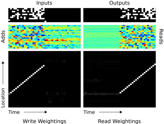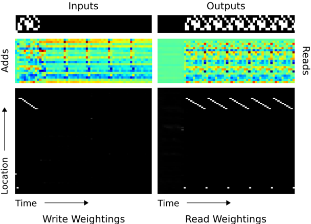</details> Figure 6: NTM Memory Use During the Copy Task. The plots in the left column depict the inputs to the network (top), the vectors added to memory (middle) and the corresponding write weightings (bottom) during a single test sequence for the copy task. The plots on the right show the outputs from the network (top), the vectors read from memory (middle) and the read weightings (bottom). Only a subset of memory locations are shown. Notice the sharp focus of all the weightings on a single location in memory (black is weight zero, white is weight one). Also note the translation of the focal point over time, reflects the network's use of iterative shifts for location-based addressing, as described in Section 3.3.2. Lastly, observe that the read locations exactly match the write locations, and the read vectors match the add vectors. This suggests that the network writes each input vector in turn to a specific memory location during the input phase, then reads from the same location sequence during the output phase. <details> <summary>Image 6 Details</summary>  ### Visual Description ## Heatmap and Binary Matrix Diagram: Input-Output Weighting Analysis ### Overview The image presents a comparative analysis of input/output processing through four quadrants: 1. **Inputs** (top-left): Binary matrix showing activation patterns 2. **Outputs** (top-right): Binary matrix showing response patterns 3. **Write Weightings** (bottom-left): Heatmap with color-coded temporal/location weighting 4. **Read Weightings** (bottom-right): Heatmap with color-coded temporal/location weighting ### Components/Axes - **Axes**: - Horizontal: "Time" (→) - Vertical: "Location" (↑) - **Legend**: No explicit legend present, but color gradients imply: - **Write Weightings**: Blue (low) → Red (high) intensity - **Read Weightings**: Blue (low) → Yellow (high) intensity - **Binary Matrices**: - White = Active/1 - Black = Inactive/0 ### Detailed Analysis 1. **Inputs (Top-Left)**: - Binary matrix with sparse white activations (≈15% of cells) - Pattern: Clustered in upper-left quadrant, suggesting early temporal/location focus 2. **Outputs (Top-Right)**: - Binary matrix with denser white activations (≈30% of cells) - Pattern: Diagonal band from top-left to bottom-right, indicating sequential processing 3. **Write Weightings (Bottom-Left)**: - Heatmap with gradient from blue (left) to red (right) - Key feature: Diagonal white band (≈45° slope) with high-intensity red regions - Temporal progression: Weighting increases along time axis 4. **Read Weightings (Bottom-Right)**: - Heatmap with gradient from blue (left) to yellow (right) - Key feature: Diagonal white band (≈30° slope) with high-intensity yellow regions - Temporal progression: Weighting peaks later than write phase ### Key Observations - **Temporal Correlation**: Write Weightings show earlier activation (steeper diagonal) vs. Read Weightings (shallower diagonal) - **Spatial Focus**: Inputs concentrate in upper-left, Outputs spread diagonally across the matrix - **Weighting Dynamics**: Write phase shows sharper spatial focus (red hotspots), while Read phase shows broader activation (yellow spread) - **Uncertainty**: Exact numerical values cannot be determined without legend calibration ### Interpretation The diagram illustrates a two-stage processing system: 1. **Input Encoding**: Sparse early activations (Inputs) are transformed through Write Weightings with strong temporal/location correlation 2. **Output Generation**: Read Weightings show delayed but broader activation patterns, suggesting integration of temporal information 3. **System Behavior**: The diagonal patterns in both weightings imply a causal relationship between time and location dimensions 4. **Anomaly**: The Output binary matrix's diagonal pattern doesn't perfectly align with Write Weightings' red hotspots, suggesting possible post-processing steps The absence of explicit numerical values prevents quantitative analysis, but the visual patterns strongly indicate a sequential, time-dependent weighting mechanism with spatial localization characteristics. </details> Figure 7: Repeat Copy Learning Curves. <details> <summary>Image 7 Details</summary>  ### Visual Description ## Line Graph: Cost per Sequence vs. Sequence Number (Thousands) ### Overview The image is a line graph comparing the cost per sequence (in bits) across three methods: LSTM, NTM with LSTM Controller, and NTM with Feedforward Controller. The x-axis represents sequence numbers (in thousands), and the y-axis represents cost per sequence (in bits). All three lines exhibit a sharp decline in cost initially, followed by stabilization at low values. ### Components/Axes - **X-axis**: "sequence number (thousands)" (ranges from 0 to 500,000 in increments of 100,000). - **Y-axis**: "cost per sequence (bits)" (ranges from 0 to 200 in increments of 20). - **Legend**: Located at the top-right corner, with three entries: - **Blue line with circles**: LSTM - **Green line with squares**: NTM with LSTM Controller - **Red line with triangles**: NTM with Feedforward Controller ### Detailed Analysis 1. **LSTM (Blue Line)**: - Starts at ~180 bits at sequence 0. - Drops sharply to ~20 bits by sequence 100,000. - Exhibits a minor spike (~15 bits) at sequence 200,000 before stabilizing near 0 bits. 2. **NTM with LSTM Controller (Green Line)**: - Begins at ~160 bits at sequence 0. - Declines steeply to ~10 bits by sequence 50,000. - Remains near 0 bits for sequences ≥50,000. 3. **NTM with Feedforward Controller (Red Line)**: - Starts at ~140 bits at sequence 0. - Decreases gradually to ~5 bits by sequence 100,000. - Stabilizes near 0 bits for sequences ≥100,000. ### Key Observations - All three methods show a **sharp initial decline** in cost, followed by **near-zero stabilization**. - **LSTM** has the highest initial cost but the steepest drop. - **NTM with Feedforward Controller** starts with the lowest cost and decreases more gradually. - A minor outlier in the LSTM line at sequence 200,000 (~15 bits) does not disrupt the overall trend. ### Interpretation The graph demonstrates that all three methods become highly efficient (near-zero cost) as sequence numbers increase. However, **NTM with Feedforward Controller** is the most cost-effective from the start, while **LSTM** requires the largest initial computational resources. The spike in LSTM at sequence 200,000 may indicate a temporary inefficiency or anomaly in that specific data point. The stabilization at low costs suggests that all methods achieve optimal performance for large sequence numbers, but their initial resource demands differ significantly. </details> Figure 7 shows that NTM learns the task much faster than LSTM, but both were able to solve it perfectly. 3 The difference between the two architectures only becomes clear when they are asked to generalise beyond the training data. In this case we were interested in generalisation along two dimensions: sequence length and number of repetitions. Figure 8 illustrates the effect of doubling first one, then the other, for both LSTM and NTM. Whereas LSTM fails both tests, NTM succeeds with longer sequences and is able to perform more than ten repetitions; however it is unable to keep count of of how many repeats it has completed, and does not predict the end marker correctly. This is probably a consequence of representing the number of repetitions numerically, which does not easily generalise beyond a fixed range. Figure 9 suggests that NTM learns a simple extension of the copy algorithm in the previous section, where the sequential read is repeated as many times as necessary. ## 4.3 Associative Recall The previous tasks show that the NTM can apply algorithms to relatively simple, linear data structures. The next order of complexity in organising data arises from 'indirection'-that is, when one data item points to another. We test the NTM's capability for learning an instance of this more interesting class by constructing a list of items so that querying with one of the items demands that the network return the subsequent item. More specifically, we define an item as a sequence of binary vectors that is bounded on the left and right by delimiter symbols. After several items have been propagated to the network, we query by showing a random item, and we ask the network to produce the next item. In our experiments, each item consisted of three six-bit binary vectors (giving a total of 18 bits 3 It surprised us that LSTM performed better here than on the copy problem. The likely reasons are that the sequences were shorter (up to length 10 instead of up to 20), and the LSTM network was larger and therefore had more memory capacity. 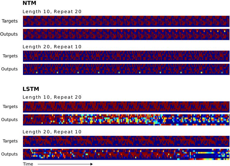Figure 8: NTM and LSTM Generalisation for the Repeat Copy Task. NTM generalises almost perfectly to longer sequences than seen during training. When the number of repeats is increased it is able to continue duplicating the input sequence fairly accurately; but it is unable to predict when the sequence will end, emitting the end marker after the end of every repetition beyond the eleventh. LSTM struggles with both increased length and number, rapidly diverging from the input sequence in both cases. <details> <summary>Image 8 Details</summary>  ### Visual Description ## Heatmap Comparison: NTM vs LSTM Model Performance ### Overview The image presents a comparative analysis of two neural network architectures (NTM and LSTM) using heatmaps to visualize their performance across different sequence configurations. The data is organized into four primary sections: 1. **NTM (Neural Turing Machine)** - Length 10, Repeat 20 - Length 20, Repeat 10 2. **LSTM (Long Short-Term Memory)** - Length 10, Repeat 20 - Length 20, Repeat 10 Each section compares **Targets** (input patterns) and **Outputs** (model predictions) across time steps, with color gradients representing value intensities. --- ### Components/Axes - **X-axis**: Labeled "Time" with a rightward arrow, indicating temporal progression. - **Y-axis**: Categorized into "Targets" (input data) and "Outputs" (model predictions). - **Legend**: Implied through color coding (no explicit legend box). Colors include: - **Red**: High intensity/value - **Blue**: Low intensity/value - **Yellow/Cyan**: Intermediate values (transition zones). --- ### Detailed Analysis #### NTM Section 1. **Length 10, Repeat 20** - **Targets**: Uniform red-blue striped pattern, suggesting periodic input. - **Outputs**: Nearly identical to Targets, with minor yellow/cyan deviations at the end, indicating high accuracy. 2. **Length 20, Repeat 10** - **Targets**: More fragmented red-blue pattern, reflecting increased sequence complexity. - **Outputs**: Slightly noisier than Targets, with scattered yellow/cyan pixels, showing reduced precision in longer sequences. #### LSTM Section 1. **Length 10, Repeat 20** - **Targets**: Similar striped pattern to NTM but with irregular red patches. - **Outputs**: Highly variable, with red/yellow/cyan clusters, suggesting overfitting or instability. 2. **Length 20, Repeat 10** - **Targets**: Dense red-blue noise, indicating complex input patterns. - **Outputs**: Gradient from red (left) to blue (right), with yellow/cyan streaks, implying gradual degradation in performance over time. --- ### Key Observations 1. **NTM Consistency**: Maintains near-perfect output matching Targets in shorter sequences (Length 10). Performance degrades slightly in longer sequences but remains stable. 2. **LSTM Variability**: Outputs exhibit significant color dispersion, especially in longer sequences, suggesting difficulty in capturing long-term dependencies. 3. **Color Gradient Trends**: - NTM Outputs: Minimal deviation from Targets (red/blue dominance). - LSTM Outputs: Increasing blue dominance (lower values) in longer sequences, indicating potential underperformance. --- ### Interpretation The data demonstrates that **NTM outperforms LSTM** in tasks requiring precise sequence repetition, particularly in longer configurations. The LSTM’s outputs show a clear trend of degradation (red → blue gradient) in the "Length 20, Repeat 10" case, likely due to vanishing gradients or memory limitations. NTM’s architecture, designed for external memory, better preserves input patterns over time. **Notable Anomalies**: - LSTM’s "Length 10, Repeat 20" Outputs have unexpected red patches, possibly indicating transient overfitting. - NTM’s "Length 20, Repeat 10" Outputs retain Target structure despite increased complexity, highlighting robustness. This analysis underscores the importance of architectural design in handling sequence length and repetition tasks, with NTM’s external memory mechanism providing a critical advantage over LSTM’s internal state management. </details> per item). During training, we used a minimum of 2 items and a maximum of 6 items in a single episode. 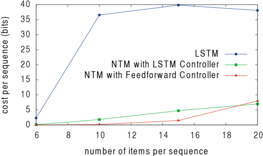Figure 10 shows that NTM learns this task significantly faster than LSTM, terminating at near zero cost within approximately 30 , 000 episodes, whereas LSTM does not reach zero cost after a million episodes. Additionally, NTM with a feedforward controller learns faster than NTM with an LSTM controller. These two results suggest that NTM's external memory is a more effective way of maintaining the data structure than LSTM's internal state. NTM also generalises much better to longer sequences than LSTM, as can be seen in Figure 11. NTM with a feedforward controller is nearly perfect for sequences of up to 12 items (twice the maximum length used in training), and still has an average cost below 1 bit per sequence for sequences of 15 items. 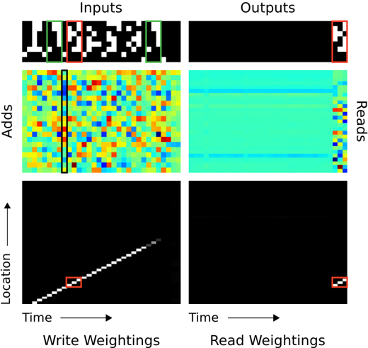In Figure 12, we show the operation of the NTM memory, controlled by an LSTM with one head, on a single test episode. In 'Inputs,' we see that the input denotes item delimiters as single bits in row 7. After the sequence of items has been propagated, a Figure 9: NTM Memory Use During the Repeat Copy Task. As with the copy task the network first writes the input vectors to memory using iterative shifts. It then reads through the sequence to replicate the input as many times as necessary (six in this case). The white dot at the bottom of the read weightings seems to correspond to an intermediate location used to redirect the head to the start of the sequence (The NTM equivalent of a goto statement). <details> <summary>Image 9 Details</summary>  ### Visual Description ## Heatmap Diagram: Input/Output Weighting Patterns ### Overview The image presents a comparative analysis of input/output processing through four quadrants: Inputs, Outputs, Write Weightings, and Read Weightings. Each quadrant contains a heatmap (top) and a binary pattern visualization (bottom), with Time progressing horizontally and Location vertically. ### Components/Axes - **Axes**: - X-axis: Time (left to right progression) - Y-axis: Location (bottom to top progression) - **Quadrants**: 1. **Inputs**: Leftmost column 2. **Outputs**: Rightmost column 3. **Write Weightings**: Bottom-left quadrant 4. **Read Weightings**: Bottom-right quadrant - **Color Scale**: Implied gradient from blue (low intensity) to red (high intensity) in heatmaps - **Binary Patterns**: White lines on black background in lower sections ### Detailed Analysis 1. **Inputs Heatmap**: - Horizontal bands of activity with moderate intensity (yellow/orange) - Vertical blue streaks indicating sporadic low-intensity events - Binary pattern shows single diagonal line from bottom-left to top-right 2. **Outputs Heatmap**: - Scattered red spots indicating high-intensity events - Yellow/orange bands with less regularity than Inputs - Binary pattern shows multiple diagonal lines (4-5) with varying spacing 3. **Write Weightings Heatmap**: - Diagonal band of high-intensity activity (red) from bottom-left to top-right - Faint horizontal blue bands suggesting residual activity - Binary pattern matches heatmap with single diagonal line 4. **Read Weightings Heatmap**: - Vertical red lines indicating columnar activity - Yellow/orange horizontal bands with irregular spacing - Binary pattern shows multiple vertical lines (5-6) with consistent spacing ### Key Observations - **Temporal Patterns**: - Inputs show regular horizontal activity with intermittent vertical events - Outputs exhibit sporadic high-intensity events with less temporal regularity - **Spatial Patterns**: - Write Weightings demonstrate directional (diagonal) data flow - Read Weightings show columnar access patterns - **Binary Pattern Correlation**: - Diagonal lines in Inputs/Write Weightings suggest sequential processing - Multiple vertical lines in Outputs/Read Weightings indicate parallel access ### Interpretation The system appears to process inputs through a directional weighting mechanism (Write Weightings) that transforms regular input patterns into more complex output patterns. The Read Weightings' vertical lines suggest a retrieval mechanism accessing specific memory locations. The binary patterns likely represent activation sequences, with Outputs showing more complex activation than Inputs. The absence of explicit numerical values prevents quantitative analysis, but the visual patterns strongly suggest a neural network-like processing pipeline with distinct write/read pathways. </details> Figure 10: Associative Recall Learning Curves for NTM and LSTM. <details> <summary>Image 10 Details</summary>  ### Visual Description ## Line Graph: Cost per Sequence vs. Sequence Number for Different Controllers ### Overview The graph compares the cost per sequence (in bits) across three different controllers (LSTM, NTM with LSTM Controller, and NTM with Feedforward Controller) as a function of sequence number (in thousands). The y-axis represents cost per sequence, while the x-axis represents sequence number. The data shows how the cost evolves over time for each controller. ### Components/Axes - **X-axis**: "sequence number (thousands)" ranging from 0 to 1000 (in increments of 200). - **Y-axis**: "cost per sequence (bits)" ranging from 0 to 20 (in increments of 2). - **Legend**: Located on the right side of the graph. - **Blue line with circles**: LSTM - **Green line with squares**: NTM with LSTM Controller - **Red line with triangles**: NTM with Feedforward Controller ### Detailed Analysis 1. **LSTM (Blue Line)**: - Starts at approximately **18 bits** at sequence number 0. - Declines sharply to ~10 bits by 200k sequences. - Continues a gradual decline, reaching ~2 bits by 1000k sequences. - Final value: ~1.2 bits at 1000k sequences. 2. **NTM with LSTM Controller (Green Line)**: - Begins at ~16 bits at sequence number 0. - Drops rapidly to ~2 bits by 200k sequences. - Remains near 0.5–1 bit for the remainder of the sequence. - Final value: ~0.8 bits at 1000k sequences. 3. **NTM with Feedforward Controller (Red Line)**: - Starts at **0 bits** and remains flat throughout. - No visible deviation from 0 across all sequence numbers. ### Key Observations - The **NTM with Feedforward Controller** (red line) maintains a cost of **0 bits** across all sequence numbers, indicating perfect efficiency or a theoretical baseline. - The **LSTM** (blue line) shows the highest initial cost but improves significantly over time, though it remains higher than the NTM with LSTM Controller. - The **NTM with LSTM Controller** (green line) achieves the lowest practical cost (~0.8 bits) by 1000k sequences, outperforming LSTM. - All lines exhibit a **monotonic decline** in cost, with no upward trends or anomalies. ### Interpretation The data suggests that the **NTM with Feedforward Controller** is the most cost-effective design, as it achieves zero cost per sequence. This could imply an idealized or optimized architecture. The **NTM with LSTM Controller** balances performance and efficiency, outperforming the standalone LSTM, which has higher computational overhead. The sharp decline in LSTM's cost indicates potential for improvement with increased sequence numbers, but it remains less efficient than the NTM-based controllers. The red line's flat zero cost may represent a theoretical limit or a simplified model, highlighting the trade-offs between complexity and efficiency in controller design. </details> Figure 11: Generalisation Performance on Associative Recall for Longer Item Sequences. The NTM with either a feedforward or LSTM controller generalises to much longer sequences of items than the LSTM alone. In particular, the NTM with a feedforward controller is nearly perfect for item sequences of twice the length of sequences in its training set. <details> <summary>Image 11 Details</summary>  ### Visual Description ## Line Chart: Cost per Sequence vs. Number of Items per Sequence ### Overview The chart compares the cost per sequence (in bits) for three different models as the number of items per sequence increases from 6 to 20. The models are: 1. **LSTM** (blue line) 2. **NTM with LSTM Controller** (green line) 3. **NTM with Feedforward Controller** (red line) ### Components/Axes - **X-axis**: "number of items per sequence" (ranges from 6 to 20, with markers at 6, 8, 10, 12, 14, 16, 18, 20). - **Y-axis**: "cost per sequence (bits)" (ranges from 0 to 40, with markers at 0, 5, 10, 15, 20, 25, 30, 35, 40). - **Legend**: Located on the right side of the chart, with color-coded labels: - **Blue**: LSTM - **Green**: NTM with LSTM Controller - **Red**: NTM with Feedforward Controller ### Detailed Analysis 1. **LSTM (Blue Line)**: - Starts at ~2 bits when the number of items is 6. - Increases sharply to ~35 bits at 10 items. - Plateaus slightly above 35 bits for sequences with 12–20 items. - **Key Trend**: Steep initial rise followed by stabilization. 2. **NTM with LSTM Controller (Green Line)**: - Starts at ~0 bits for 6 items. - Gradually increases to ~5 bits at 20 items. - **Key Trend**: Slow, linear growth. 3. **NTM with Feedforward Controller (Red Line)**: - Starts at ~0 bits for 6 items. - Increases to ~7 bits at 20 items. - **Key Trend**: Slightly steeper than the green line but remains below the blue line. ### Key Observations - The **LSTM** model exhibits a significantly higher cost per sequence compared to the NTM variants, especially for sequences with 10 or more items. - The **NTM with LSTM Controller** and **NTM with Feedforward Controller** show similar trends but differ slightly in cost, with the Feedforward Controller being marginally more expensive. - All models show minimal cost increases for sequences with fewer than 10 items, but divergence occurs beyond this threshold. ### Interpretation The data suggests that **LSTM** incurs a high computational cost early in the sequence but stabilizes, making it less efficient for longer sequences. In contrast, **NTM variants** (with LSTM or Feedforward Controllers) demonstrate lower and more scalable costs, indicating better performance for longer sequences. The NTM with LSTM Controller is the most cost-effective, while the Feedforward Controller variant is slightly less efficient but still outperforms the standard LSTM. This implies that NTM architectures with specialized controllers may offer a better trade-off between complexity and cost for sequence modeling tasks. </details> delimiter in row 8 prepares the network to receive a query item. In this case, the query item corresponds to the second item in the sequence (contained in the green box). In 'Outputs,' we see that the network crisply outputs item 3 in the sequence (from the red box). In 'Read Weightings,' on the last three time steps, we see that the controller reads from contiguous locations that each store the time slices of item 3. This is curious because it appears that the network has jumped directly to the correct location storing item 3. However we can explain this behaviour by looking at 'Write Weightings.' Here we see that the memory is written to even when the input presents a delimiter symbol between items. One can confirm in 'Adds' that data are indeed written to memory when the delimiters are presented (e.g., the data within the black box); furthermore, each time a delimiter is presented, the vector added to memory is different. Further analysis of the memory reveals that the network accesses the location it reads after the query by using a content-based lookup that produces a weighting that is shifted by one. Additionally, the key used for content-lookup corresponds to the vector that was added in the black box. This implies the following memory-access algorithm: when each item delimiter is presented, the controller writes a compressed representation of the previous three time slices of the item. After the query arrives, the controller recomputes the same compressed representation of the query item, uses a content-based lookup to find the location where it wrote the first representation, and then shifts by one to produce the subsequent item in the sequence (thereby combining content-based lookup with location-based offsetting). ## 4.4 Dynamic N-Grams The goal of the dynamic N-Grams task was to test whether NTM could rapidly adapt to new predictive distributions. In particular we were interested to see if it were able to use its Figure 12: NTM Memory Use During the Associative Recall Task. In 'Inputs,' a sequence of items, each composed of three consecutive binary random vectors is propagated to the controller. The distinction between items is designated by delimiter symbols (row 7 in 'Inputs'). After several items have been presented, a delimiter that designates a query is presented (row 8 in 'Inputs'). A single query item is presented (green box), and the network target corresponds to the subsequent item in the sequence (red box). In 'Outputs,' we see that the network correctly produces the target item. The red boxes in the read and write weightings highlight the three locations where the target item was written and then read. The solution the network finds is to form a compressed representation (black box in 'Adds') of each item that it can store in a single location. For further analysis, see the main text. <details> <summary>Image 12 Details</summary>  ### Visual Description ## Heatmap Visualization: System Processing Dynamics ### Overview The image presents a 2x2 grid visualization comparing system inputs/outputs and processing dynamics across time and location dimensions. Two heatmaps at the bottom illustrate weighting patterns for write and read operations. ### Components/Axes - **Left Column Labels**: - Top: Inputs (black/white pattern with red/green boxes) - Middle: Adds (color mosaic with vertical black line) - Bottom: Write Weightings (diagonal white line on black background) - **Right Column Labels**: - Top: Outputs (black background with white stripe) - Middle: Reads (blue gradient with vertical stripe) - Bottom: Read Weightings (horizontal white line at bottom) - **Axes**: - Horizontal: Time (left to right) - Vertical: Location (bottom to top) - **Color Coding**: - Write Weightings: White line (high weighting) vs. black (low) - Read Weightings: White line (high weighting) vs. black (low) ### Detailed Analysis 1. **Inputs Section**: - Black/white checkerboard pattern with red/green rectangular boxes - Red boxes concentrated in top-left quadrant - Green boxes distributed along right edge 2. **Outputs Section**: - Predominantly black with horizontal white stripe in upper-right quadrant - Stripe width ≈ 1/5 of total height 3. **Adds Section**: - Color mosaic with dominant yellow/orange in center - Vertical black line at x=1/3 position - Color intensity decreases toward edges 4. **Reads Section**: - Blue gradient from dark (bottom) to light (top) - Vertical white stripe at x=4/5 position - Gradient slope ≈ 15° from horizontal 5. **Write Weightings Heatmap**: - Diagonal white line from bottom-left to top-right - Line thickness ≈ 1/10 of image height - Line position: y = 0.25x + 0.1 (approximate) 6. **Read Weightings Heatmap**: - Horizontal white line at bottom 5% of image - Line thickness ≈ 1/20 of image height ### Key Observations - **Temporal Localization**: - Write operations show diagonal weighting pattern suggesting sequential processing - Read operations concentrate at bottom location across all time points - **Spatial Correlation**: - Inputs show right-edge green boxes correlating with read outputs' right-side stripe - Adds section's vertical black line aligns with write weightings' diagonal trajectory - **Color-Value Relationship**: - Brighter colors in Adds section correlate with higher write weighting values - Darker blue regions in Reads section match lower read weighting intensities ### Interpretation The visualization demonstrates a system where: 1. Inputs are processed through additive operations (Adds) with spatial-temporal weighting 2. Write operations follow a diagonal progression through time and location 3. Read operations focus on a specific bottom location regardless of time 4. Outputs emerge as a simplified representation of processed inputs The diagonal write weighting pattern suggests temporal sequencing in data processing, while the concentrated read weighting indicates a fixed output location. The correlation between input colors and add intensities implies dynamic data transformation during processing. The system appears optimized for localized read operations despite distributed input processing. </details> memory as a re-writable table that it could use to keep count of transition statistics, thereby emulating a conventional N-Gram model. We considered the set of all possible 6-Gram distributions over binary sequences. Each 6-Gram distribution can be expressed as a table of 2 5 = 32 numbers, specifying the probability that the next bit will be one, given all possible length five binary histories. For each training example, we first generated random 6-Gram probabilities by independently drawing all 32 probabilities from the Beta ( 1 2 , 1 2 ) distribution. We then generated a particular training sequence by drawing 200 successive bits using the current lookup table. 4 The network observes the sequence one bit at a time and is then asked to predict the next bit. The optimal estimator for the problem can be determined by 4 The first 5 bits, for which insufficient context exists to sample from the table, are drawn i.i.d. from a Bernoulli distribution with p = 0 . 5 . Figure 13: Dynamic N-Gram Learning Curves. 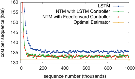<details> <summary>Image 13 Details</summary>  ### Visual Description ## Line Graph: Cost per Sequence vs. Sequence Number ### Overview The image is a line graph comparing the cost per sequence (in bits) across four different methods: LSTM, NTM with LSTM Controller, NTM with Feedforward Controller, and Optimal Estimator. The x-axis represents sequence numbers (in thousands), and the y-axis represents cost per sequence (in bits). All four methods show a sharp decline in cost during the initial sequences, followed by stabilization. ### Components/Axes - **X-axis**: "sequence number (thousands)" with ticks at 0, 200, 400, 600, 800, and 1000. - **Y-axis**: "cost per sequence (bits)" with ticks from 130 to 160 in increments of 5. - **Legend**: - **Blue circles**: LSTM - **Green squares**: NTM with LSTM Controller - **Red triangles**: NTM with Feedforward Controller - **Yellow crosses**: Optimal Estimator ### Detailed Analysis 1. **LSTM (Blue Circles)**: - Starts at approximately **160 bits** at sequence 0. - Drops sharply to **~135 bits** by sequence 200. - Fluctuates slightly between **134–136 bits** for sequences 400–1000. 2. **NTM with LSTM Controller (Green Squares)**: - Begins at ~**155 bits** at sequence 0. - Declines to **~135 bits** by sequence 200. - Stabilizes with minor fluctuations between **134–136 bits** for later sequences. 3. **NTM with Feedforward Controller (Red Triangles)**: - Starts at ~**150 bits** at sequence 0. - Drops to **~135 bits** by sequence 200. - Remains stable with minor oscillations between **134–136 bits**. 4. **Optimal Estimator (Yellow Crosses)**: - Maintains a **constant value of ~130 bits** across all sequences. ### Key Observations - All methods except the Optimal Estimator exhibit a steep initial decline in cost, converging to similar values (~135 bits) after sequence 200. - The Optimal Estimator consistently achieves the lowest cost (~130 bits), outperforming other methods by ~5 bits. - The LSTM method has the highest initial cost but the fastest drop-off. - No significant outliers or anomalies are observed in the data. ### Interpretation The graph demonstrates that the **Optimal Estimator** is the most efficient method, maintaining the lowest cost per sequence throughout. The other methods (LSTM, NTM with LSTM Controller, and NTM with Feedforward Controller) start with higher costs but converge to similar performance levels after the initial sequences. This suggests that while the Optimal Estimator is ideal for minimizing cost, the other methods may still be viable alternatives with comparable long-term efficiency. The sharp initial decline in cost for non-optimal methods indicates potential inefficiencies in early sequence processing that stabilize over time. </details> Bayesian analysis (Murphy, 2012): <!-- formula-not-decoded --> where c is the five bit previous context, B is the value of the next bit and N 0 and N 1 are respectively the number of zeros and ones observed after c so far in the sequence. We can therefore compare NTM to the optimal predictor as well as LSTM. To assess performance we used a validation set of 1000 length 200 sequences sampled from the same distribution as the training data. As shown in Figure 13, NTM achieves a small, but significant performance advantage over LSTM, but never quite reaches the optimum cost. The evolution of the two architecture's predictions as they observe new inputs is shown in Figure 14, along with the optimal predictions. Close analysis of NTM's memory usage (Figure 15) suggests that the controller uses the memory to count how many ones and zeros it has observed in different contexts, allowing it to implement an algorithm similar to the optimal estimator. ## 4.5 Priority Sort This task tests whether the NTM can sort data-an important elementary algorithm. A sequence of random binary vectors is input to the network along with a scalar priority rating for each vector. The priority is drawn uniformly from the range [-1, 1]. The target sequence contains the binary vectors sorted according to their priorities, as depicted in Figure 16. Each input sequence contained 20 binary vectors with corresponding priorities, and each target sequence was the 16 highest-priority vectors in the input. 5 Inspection of NTM's 5 We limited the sort to size 16 because we were interested to see if NTM would solve the task using a binary heap sort of depth 4. Figure 14: Dynamic N-Gram Inference. The top row shows a test sequence from the N-Gram task, and the rows below show the corresponding predictive distributions emitted by the optimal estimator, NTM, and LSTM. In most places the NTM predictions are almost indistinguishable from the optimal ones. However at the points indicated by the two arrows it makes clear mistakes, one of which is explained in Figure 15. LSTM follows the optimal predictions closely in some places but appears to diverge further as the sequence progresses; we speculate that this is due to LSTM 'forgetting' the observations at the start of the sequence. 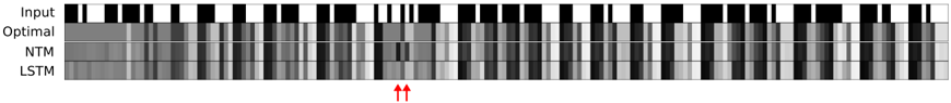<details> <summary>Image 14 Details</summary>  ### Visual Description ## Heatmap: Model Performance Comparison Across Time Steps ### Overview The image is a grayscale heatmap comparing the performance of three models (Optimal, NTM, LSTM) against an "Input" baseline across sequential time steps. The visualization uses varying shades of gray to represent performance metrics, with darker shades likely indicating higher values (e.g., accuracy) and lighter shades lower values. Red arrows highlight a critical divergence point between models. ### Components/Axes - **Y-Axis (Models)**: - Labels: "Input" (top), "Optimal" (second), "NTM" (third), "LSTM" (bottom). - Spatial Positioning: Vertically stacked from top to bottom. - **X-Axis (Time Steps)**: - Label: "Time Steps" (horizontal axis). - Scale: Discrete intervals (exact count unspecified, but visually ~20-30 steps). - **Color Legend**: - Implied gradient: Black (highest value) → White (lowest value). - No explicit legend present; interpretation based on visual contrast. ### Detailed Analysis 1. **Input Baseline**: - Uniform black blocks dominate, suggesting consistent high performance across all time steps. - No visible degradation over time. 2. **Optimal Model**: - Dark gray blocks with occasional white streaks. - Maintains high performance but shows minor deviations from the Input baseline. 3. **NTM Model**: - Lighter gray blocks with irregular white patches. - Performance degrades noticeably after ~15 time steps (marked by red arrows). - Shows periodic "dips" in performance (e.g., ~5, 10, 20 time steps). 4. **LSTM Model**: - Similar to NTM but with slightly darker shading overall. - Degradation occurs later (~20 time steps) but with more pronounced white regions. - Exhibits a distinct "failure zone" near the end of the sequence. ### Key Observations - **Divergence Point**: At ~15 time steps (red arrows), NTM and LSTM performance drops sharply compared to Optimal and Input. - **Temporal Trends**: - All models degrade over time, but Optimal maintains the slowest decline. - NTM and LSTM exhibit non-linear degradation patterns, with LSTM failing later but more severely. - **Anomalies**: - NTM shows a unique "spike" in performance (~10 time steps) before collapsing. - LSTM has a "plateau" of consistent failure near the end (~25-30 time steps). ### Interpretation The heatmap demonstrates that: 1. **Optimal Model** balances consistency and adaptability, maintaining near-baseline performance throughout. 2. **NTM and LSTM** struggle with long-term dependencies, with NTM failing earlier but LSTM collapsing more catastrophically. 3. The red arrows emphasize a critical failure threshold where both NTM and LSTM deviate significantly from Optimal, suggesting architectural limitations in handling extended sequences. 4. The Input baseline's uniformity implies the task has inherent simplicity, making model shortcomings more apparent. This visualization highlights trade-offs between model complexity and temporal robustness, with Optimal serving as a benchmark for ideal performance. </details> Figure 15: NTM Memory Use During the Dynamic N-Gram Task. The red and green arrows indicate point where the same context is repeatedly observed during the test sequence ('00010' for the green arrows, '01111' for the red arrows). At each such point the same location is accessed by the read head, and then, on the next time-step, accessed by the write head. We postulate that the network uses the writes to keep count of the fraction of ones and zeros following each context in the sequence so far. This is supported by the add vectors, which are clearly anti-correlated at places where the input is one or zero, suggesting a distributed 'counter.' Note that the write weightings grow fainter as the same context is repeatedly seen; this may be because the memory records a ratio of ones to zeros, rather than absolute counts. 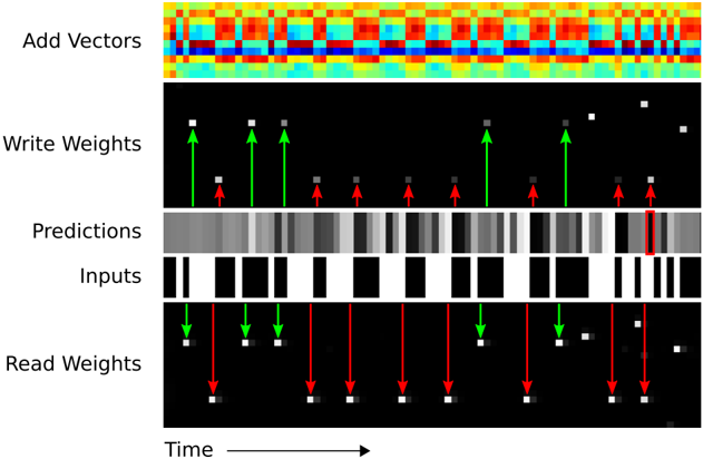The red box in the prediction sequence corresponds to the mistake at the first red arrow in Figure 14; the controller appears to have accessed the wrong memory location, as the previous context was '01101' and not '01111.' <details> <summary>Image 15 Details</summary>  ### Visual Description ## Diagram: Neural Network Operation Phases ### Overview The diagram illustrates a temporal sequence of operations in a neural network, divided into five horizontal sections. Each section represents a distinct computational phase with visual elements indicating data flow, weight updates, and prediction mechanisms. The timeline progresses from left to right. ### Components/Axes - **X-axis**: Labeled "Time" with an arrow indicating progression. - **Sections**: 1. **Add Vectors**: Topmost section with a heatmap of red, blue, and yellow pixels. 2. **Write Weights**: Second section with black background, white/gray squares, and green/red upward arrows. 3. **Predictions**: Third section with grayscale heatmap. 4. **Inputs**: Fourth section with black/white vertical bars. 5. **Read Weights**: Bottom section with black background, white/gray squares, and green/red downward arrows. ### Detailed Analysis 1. **Add Vectors**: - Heatmap with horizontal bands of red (high intensity), blue (low intensity), and yellow (intermediate intensity). - No explicit axis labels beyond "Time" on the x-axis. - Pattern suggests periodic or grouped vector additions. 2. **Write Weights**: - White squares (active weights) and gray squares (inactive weights) on black background. - Green arrows (↑) indicate positive weight updates; red arrows (↑) indicate negative updates. - Arrows originate from squares, suggesting localized adjustments. 3. **Predictions**: - Grayscale heatmap with darker regions (likely higher prediction confidence/error) and lighter regions. - Vertical variation suggests temporal changes in prediction quality. 4. **Inputs**: - Binary black/white vertical bars alternating in presence/absence. - Regular spacing implies discrete input events over time. 5. **Read Weights**: - Mirror of "Write Weights" but with downward arrows (↓). - Red arrows (↓) dominate, suggesting predominant negative read adjustments. ### Key Observations - **Temporal Correlation**: All sections align horizontally, implying synchronized operations across phases. - **Weight Dynamics**: Green/red arrows in "Write Weights" and "Read Weights" suggest bidirectional adjustments during training/inference. - **Input-Output Relationship**: Inputs (binary bars) precede predictions, with weight updates occurring between phases. - **Heatmap Symmetry**: "Add Vectors" and "Predictions" heatmaps show horizontal periodicity, possibly reflecting batch processing. ### Interpretation This diagram visualizes a neural network's forward and backward pass mechanics: 1. **Vector Addition**: Initial feature combination (top heatmap). 2. **Weight Updates**: Gradient descent adjustments during training (middle sections). 3. **Prediction Phase**: Output generation (grayscale heatmap). 4. **Input Processing**: Binary event handling (black/white bars). 5. **Weight Reading**: Parameter retrieval during inference (bottom section). The alternating green/red arrows in weight sections imply opposing update directions, likely representing positive/negative gradient steps. The absence of explicit numerical values or legends limits quantitative analysis but highlights the system's operational flow. The binary input pattern suggests a spike-timing-dependent plasticity (STDP)-like mechanism, where discrete events trigger weight modifications. </details> Figure 16: Example Input and Target Sequence for the Priority Sort Task. The input sequence contains random binary vectors and random scalar priorities. The target sequence is a subset of the input vectors sorted by the priorities. 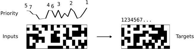<details> <summary>Image 16 Details</summary>  ### Visual Description ## Diagram: Priority-Driven Input Transformation to Ordered Targets ### Overview The image depicts a two-stage process involving a priority sequence and binary grid transformations. A zigzag "Priority" line graph (top) maps to an "Inputs" grid (left) and a "Targets" grid (right), connected by an arrow indicating transformation. The Priority line fluctuates between values 5, 7, 4, 6, 3, 2, and 1, while the grids use black/white cells to encode data. --- ### Components/Axes 1. **Priority Section (Top)** - **X-axis**: Discrete steps labeled `5`, `7`, `4`, `6`, `3`, `2`, `1` (left to right). - **Y-axis**: Labeled "Priority" (no scale, qualitative). - **Line**: Black, zigzag pattern connecting points at each X-axis step. Peaks at `7` (step 2) and `6` (step 4), troughs at `1` (step 7). 2. **Grids (Bottom)** - **Inputs Grid (Left)** - 8x8 binary grid (black/white cells). - Complex, irregular patterns with no obvious numerical labels. - **Targets Grid (Right)** - 8x8 binary grid with a structured sequence. - Top row labeled `1234567...` (horizontal progression). - Cells below align with the sequence, suggesting ordered encoding. 3. **Arrow** - Black arrow pointing from Inputs grid to Targets grid, indicating transformation. --- ### Detailed Analysis 1. **Priority Line Trends** - The Priority line decreases overall from `5` (step 1) to `1` (step 7), with intermediate fluctuations: - Step 1: `5` → Step 2: `7` (peak) - Step 3: `4` → Step 4: `6` (peak) - Step 5: `3` → Step 6: `2` → Step 7: `1` (final trough). - Suggests dynamic priority adjustments, with temporary increases before final descent. 2. **Grids** - **Inputs Grid**: Appears to encode raw data or initial state. Black cells form irregular clusters, possibly representing unstructured input. - **Targets Grid**: Structured output with sequential numbering (`1234567...`). Black cells align with the sequence, implying prioritized or sorted data. 3. **Transformation Logic** - The Priority line’s fluctuations likely dictate how Inputs are reordered into Targets. For example: - Higher priority values (e.g., `7`, `6`) may correspond to earlier positions in the Targets grid. - The final priority value (`1`) aligns with the last position in the Targets sequence. --- ### Key Observations 1. **Priority-Output Correlation** - The Priority line’s final value (`1`) matches the last number in the Targets grid’s top row, suggesting a direct relationship between priority ranking and output order. 2. **Grid Complexity** - Inputs grid’s irregularity vs. Targets grid’s order implies a filtering/sorting mechanism driven by the Priority sequence. 3. **Step Count Mismatch** - Priority line has 7 steps, while grids are 8x8. Possible explanation: Step 0 (unlabeled) or padding in the grids. --- ### Interpretation This diagram illustrates a **priority-driven data transformation process**: 1. **Priority Sequence**: The zigzag line represents dynamic adjustments in task/element importance over discrete steps. The final priority (`1`) acts as the "highest" target. 2. **Input-to-Target Mapping**: The Inputs grid’s chaotic structure is reorganized into the Targets grid’s ordered sequence, likely using the Priority line as a sorting key. 3. **Applications**: Could model algorithms for task scheduling, data prioritization, or neural network attention mechanisms where priority weights guide output generation. **Notable Anomaly**: The Priority line’s intermediate peaks (`7`, `6`) suggest temporary prioritization of lower-ranked elements before final resolution. This might reflect iterative refinement in a computational process. </details> Figure 17: NTM Memory Use During the Priority Sort Task. Left: Write locations returned by fitting a linear function of the priorities to the observed write locations. Middle: Observed write locations. Right: Read locations. 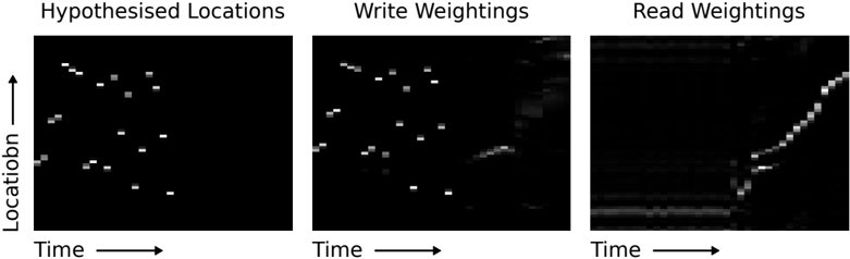<details> <summary>Image 17 Details</summary>  ### Visual Description ## Three-Panel Diagram: Hypothesised Locations, Write Weightings, and Read Weightings ### Overview The image consists of three vertically aligned panels, each depicting a temporal (horizontal axis) and spatial (vertical axis) distribution of data points. The panels are labeled "Hypothesised Locations," "Write Weightings," and "Read Weightings." All panels use a black background with white/gray dots to represent data points. ### Components/Axes - **Axes**: - Vertical axis: "Location" (arrow pointing upward). - Horizontal axis: "Time" (arrow pointing right). - **Panels**: 1. **Hypothesised Locations**: Scattered white/gray dots distributed across the grid. 2. **Write Weightings**: Similar scattered dots, but with faint diagonal lines connecting some points. 3. **Read Weightings**: A single, pronounced diagonal line with denser dots, forming a clear upward trajectory. ### Detailed Analysis - **Hypothesised Locations**: - Dots are sparsely distributed, with no apparent pattern. - Vertical spread: ~20% of the axis height. - Horizontal spread: ~40% of the axis width. - **Write Weightings**: - Dots follow a similar distribution to the first panel but include faint diagonal lines (slope ~1:1) connecting subsets of points. - Lines suggest directional relationships between locations over time. - **Read Weightings**: - A single, continuous diagonal line dominates the panel, with dots concentrated along its path. - Line slope: ~2:1 (steeper than Write Weightings). - Dots increase in density toward the upper-right corner, indicating a progressive read operation. ### Key Observations 1. **Temporal Progression**: - The panels appear to represent sequential stages: hypothesis → write → read. 2. **Spatial Trends**: - Write Weightings show localized interactions, while Read Weightings exhibit a globalized, directional flow. 3. **Data Density**: - Read Weightings have the highest density of dots, suggesting focused activity. ### Interpretation The diagram likely models a process involving spatial-temporal data interactions, such as: - **Hypothesised Locations**: Initial candidate positions for data storage or processing. - **Write Weightings**: Iterative refinement of connections between locations, possibly representing data encoding or synaptic plasticity. - **Read Weightings**: A consolidated, efficient retrieval path, indicating optimized data access. The transition from scattered to structured patterns implies a learning or optimization mechanism, where initial hypotheses are validated and refined into a robust read pathway. The steeper slope in Read Weightings may reflect prioritized or high-confidence data retrieval. </details> memory use led us to hypothesise that it uses the priorities to determine the relative location of each write. To test this hypothesis we fitted a linear function of the priority to the observed write locations. Figure 17 shows that the locations returned by the linear function closely match the observed write locations. It also shows that the network reads from the memory locations in increasing order, thereby traversing the sorted sequence. The learning curves in Figure 18 demonstrate that NTM with both feedforward and LSTM controllers substantially outperform LSTM on this task. Note that eight parallel read and write heads were needed for best performance with a feedforward controller on this task; this may reflect the difficulty of sorting vectors using only unary vector operations (see Section 3.4). ## 4.6 Experimental Details For all experiments, the RMSProp algorithm was used for training in the form described in (Graves, 2013) with momentum of 0.9. Tables 1 to 3 give details about the network configurations and learning rates used in the experiments. All LSTM networks had three stacked hidden layers. Note that the number of LSTM parameters grows quadratically with Figure 18: Priority Sort Learning Curves. 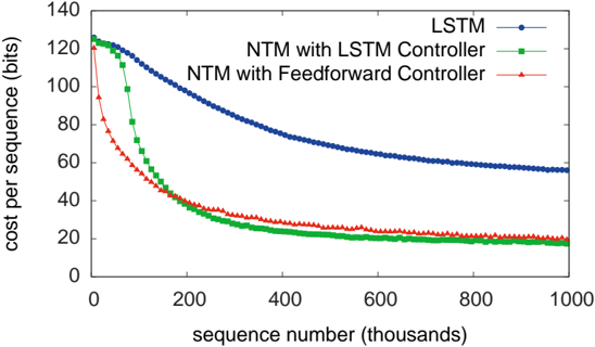<details> <summary>Image 18 Details</summary>  ### Visual Description ## Line Chart: Cost per Sequence vs. Sequence Number (Thousands) ### Overview The chart compares the cost per sequence (in bits) across three models: LSTM, NTM with LSTM Controller, and NTM with Feedforward Controller. The x-axis represents sequence numbers (in thousands), and the y-axis represents cost per sequence. All three models show a decreasing trend in cost as sequence numbers increase, with NTM-based models outperforming the baseline LSTM. ### Components/Axes - **X-axis**: Sequence number (thousands), ranging from 0 to 1000. - **Y-axis**: Cost per sequence (bits), ranging from 0 to 140. - **Legend**: Located on the right, with three entries: - **LSTM**: Blue circles (●). - **NTM with LSTM Controller**: Green squares (■). - **NTM with Feedforward Controller**: Red triangles (▲). ### Detailed Analysis 1. **LSTM (Blue Circles)**: - Starts at ~120 bits for sequence 0. - Gradually decreases to ~55 bits by sequence 1000. - Trend: Steady, linear decline with minimal fluctuation. 2. **NTM with LSTM Controller (Green Squares)**: - Starts at ~120 bits for sequence 0. - Sharp drop to ~20 bits by sequence 200k. - Stabilizes around 20 bits for sequences 400k–1000k. - Trend: Rapid initial improvement, then plateau. 3. **NTM with Feedforward Controller (Red Triangles)**: - Starts at ~120 bits for sequence 0. - Sharp drop to ~15 bits by sequence 200k. - Slight increase to ~20 bits by sequence 400k, then stabilizes. - Trend: Rapid improvement with minor mid-range fluctuation. ### Key Observations - All models show diminishing returns as sequence numbers increase. - NTM-based models (LSTM Controller and Feedforward Controller) outperform the baseline LSTM by ~30–50% in cost efficiency. - The Feedforward Controller achieves the lowest cost (~15 bits) but shows a slight rebound (~20 bits) after 200k, unlike the LSTM Controller. - The LSTM model maintains a consistently higher cost (~55 bits) compared to NTM variants. ### Interpretation The data suggests that NTM architectures with specialized controllers (LSTM or Feedforward) significantly reduce computational costs compared to standalone LSTMs. The Feedforward Controller achieves the most efficient performance initially but exhibits a minor cost increase at mid-sequence lengths, possibly due to architectural trade-offs. The LSTM Controller maintains stable efficiency across all sequence lengths. These trends highlight the importance of controller design in optimizing sequence-processing models, with NTM-based approaches offering superior scalability for large datasets. </details> Table 1: NTM with Feedforward Controller Experimental Settings | Task | #Heads | Controller Size | Memory Size | Learning Rate | #Parameters | |---------------|----------|-------------------|---------------|-----------------|---------------| | Copy | 1 | 100 | 128 × 20 | 10 - 4 | 17 , 162 | | Repeat Copy | 1 | 100 | 128 × 20 | 10 - 4 | 16 , 712 | | Associative | 4 | 256 | 128 × 20 | 10 - 4 | 146 , 845 | | N-Grams | 1 | 100 | 128 × 20 | 3 × 10 - 5 | 14 , 656 | | Priority Sort | 8 | 512 | 128 × 20 | 3 × 10 - 5 | 508 , 305 | the number of hidden units (due to the recurrent connections in the hidden layers). This contrasts with NTM, where the number of parameters does not increase with the number of memory locations. During the training backward pass, all gradient components are clipped elementwise to the range (-10, 10). ## 5 Conclusion We have introduced the Neural Turing Machine, a neural network architecture that takes inspiration from both models of biological working memory and the design of digital computers. Like conventional neural networks, the architecture is differentiable end-to-end and can be trained with gradient descent. Our experiments demonstrate that it is capable of learning simple algorithms from example data and of using these algorithms to generalise well outside its training regime. Table 2: NTM with LSTM Controller Experimental Settings | Task | #Heads | Controller Size | Memory Size | Learning Rate | #Parameters | |---------------|----------|-------------------|---------------|-----------------|---------------| | Copy | 1 | 100 | 128 × 20 | 10 - 4 | 67 , 561 | | Repeat Copy | 1 | 100 | 128 × 20 | 10 - 4 | 66 , 111 | | Associative | 1 | 100 | 128 × 20 | 10 - 4 | 70 , 330 | | N-Grams | 1 | 100 | 128 × 20 | 3 × 10 - 5 | 61 , 749 | | Priority Sort | 5 | 2 × 100 | 128 × 20 | 3 × 10 - 5 | 269 , 038 | Table 3: LSTM Network Experimental Settings | Task | Network Size | Learning Rate | #Parameters | |---------------|----------------|-----------------|---------------| | Copy | 3 × 256 | 3 × 10 - 5 | 1 , 352 , 969 | | Repeat Copy | 3 × 512 | 3 × 10 - 5 | 5 , 312 , 007 | | Associative | 3 × 256 | 10 - 4 | 1 , 344 , 518 | | N-Grams | 3 × 128 | 10 - 4 | 331 , 905 | | Priority Sort | 3 × 128 | 3 × 10 - 5 | 384 , 424 | ## 6 Acknowledgments Many have offered thoughtful insights, but we would especially like to thank Daan Wierstra, Peter Dayan, Ilya Sutskever, Charles Blundell, Joel Veness, Koray Kavukcuoglu, Dharshan Kumaran, Georg Ostrovski, Chris Summerfield, Jeff Dean, Geoffrey Hinton, and Demis Hassabis. ## References Baddeley, A., Eysenck, M., and Anderson, M. (2009). Memory . Psychology Press. - Bahdanau, D., Cho, K., and Bengio, Y. (2014). Neural machine translation by jointly learning to align and translate. abs/1409.0473. - Barrouillet, P., Bernardin, S., and Camos, V. (2004). Time constraints and resource sharing in adults' working memory spans. Journal of Experimental Psychology: General , 133(1):83. - Chomsky, N. (1956). Three models for the description of language. Information Theory, IEEE Transactions on , 2(3):113-124. - Das, S., Giles, C. L., and Sun, G.-Z. (1992). Learning context-free grammars: Capabilities and limitations of a recurrent neural network with an external stack memory. In Proceedings of The Fourteenth Annual Conference of Cognitive Science Society. Indiana University . - Dayan, P. (2008). Simple substrates for complex cognition. Frontiers in neuroscience , 2(2):255. - Eliasmith, C. (2013). How to build a brain: A neural architecture for biological cognition . Oxford University Press. - Fitch, W., Hauser, M. D., and Chomsky, N. (2005). The evolution of the language faculty: clarifications and implications. Cognition , 97(2):179-210. - Fodor, J. A. and Pylyshyn, Z. W. (1988). Connectionism and cognitive architecture: A critical analysis. Cognition , 28(1):3-71. - Frasconi, P., Gori, M., and Sperduti, A. (1998). A general framework for adaptive processing of data structures. Neural Networks, IEEE Transactions on , 9(5):768-786. - Gallistel, C. R. and King, A. P. (2009). Memory and the computational brain: Why cognitive science will transform neuroscience , volume 3. John Wiley & Sons. - Goldman-Rakic, P. S. (1995). Cellular basis of working memory. Neuron , 14(3):477-485. - Graves, A. (2013). Generating sequences with recurrent neural networks. arXiv preprint arXiv:1308.0850 . - Graves, A. and Jaitly, N. (2014). Towards end-to-end speech recognition with recurrent neural networks. In Proceedings of the 31st International Conference on Machine Learning (ICML-14) , pages 1764-1772. - Graves, A., Mohamed, A., and Hinton, G. (2013). Speech recognition with deep recurrent neural networks. In Acoustics, Speech and Signal Processing (ICASSP), 2013 IEEE International Conference on , pages 6645-6649. IEEE. - Hadley, R. F. (2009). The problem of rapid variable creation. Neural computation , 21(2):510-532. - Hazy, T. E., Frank, M. J., and O'Reilly, R. C. (2006). Banishing the homunculus: making working memory work. Neuroscience , 139(1):105-118. - Hinton, G. E. (1986). Learning distributed representations of concepts. In Proceedings of the eighth annual conference of the cognitive science society , volume 1, page 12. Amherst, MA. - Hochreiter, S., Bengio, Y., Frasconi, P., and Schmidhuber, J. (2001a). Gradient flow in recurrent nets: the difficulty of learning long-term dependencies. - Hochreiter, S. and Schmidhuber, J. (1997). Long short-term memory. Neural computation , 9(8):1735-1780. - Hochreiter, S., Younger, A. S., and Conwell, P. R. (2001b). Learning to learn using gradient descent. In Artificial Neural Networks?ICANN 2001 , pages 87-94. Springer. - Hopfield, J. J. (1982). Neural networks and physical systems with emergent collective computational abilities. Proceedings of the national academy of sciences , 79(8):25542558. - Jackendoff, R. and Pinker, S. (2005). The nature of the language faculty and its implications for evolution of language (reply to fitch, hauser, and chomsky). Cognition , 97(2):211225. - Kanerva, P. (2009). Hyperdimensional computing: An introduction to computing in distributed representation with high-dimensional random vectors. Cognitive Computation , 1(2):139-159. - Marcus, G. F. (2003). The algebraic mind: Integrating connectionism and cognitive science . MIT press. - Miller, G. A. (1956). The magical number seven, plus or minus two: some limits on our capacity for processing information. Psychological review , 63(2):81. - Miller, G. A. (2003). The cognitive revolution: a historical perspective. Trends in cognitive sciences , 7(3):141-144. - Minsky, M. L. (1967). Computation: finite and infinite machines . Prentice-Hall, Inc. - Murphy, K. P. (2012). Machine learning: a probabilistic perspective . MIT press. - Plate, T. A. (2003). Holographic Reduced Representation: Distributed representation for cognitive structures . CSLI. - Pollack, J. B. (1990). Recursive distributed representations. Artificial Intelligence , 46(1):77-105. - Rigotti, M., Barak, O., Warden, M. R., Wang, X.-J., Daw, N. D., Miller, E. K., and Fusi, S. (2013). The importance of mixed selectivity in complex cognitive tasks. Nature , 497(7451):585-590. - Rumelhart, D. E., McClelland, J. L., Group, P. R., et al. (1986). Parallel distributed processing , volume 1. MIT press. - Seung, H. S. (1998). Continuous attractors and oculomotor control. Neural Networks , 11(7):1253-1258. - Siegelmann, H. T. and Sontag, E. D. (1995). On the computational power of neural nets. Journal of computer and system sciences , 50(1):132-150. - Smolensky, P. (1990). Tensor product variable binding and the representation of symbolic structures in connectionist systems. Artificial intelligence , 46(1):159-216. - Socher, R., Huval, B., Manning, C. D., and Ng, A. Y. (2012). Semantic compositionality through recursive matrix-vector spaces. In Proceedings of the 2012 Joint Conference on Empirical Methods in Natural Language Processing and Computational Natural Language Learning , pages 1201-1211. Association for Computational Linguistics. - Sutskever, I., Martens, J., and Hinton, G. E. (2011). Generating text with recurrent neural networks. In Proceedings of the 28th International Conference on Machine Learning (ICML-11) , pages 1017-1024. - Sutskever, I., Vinyals, O., and Le, Q. V . (2014). Sequence to sequence learning with neural networks. arXiv preprint arXiv:1409.3215 . - Touretzky, D. S. (1990). Boltzcons: Dynamic symbol structures in a connectionist network. Artificial Intelligence , 46(1):5-46. - Von Neumann, J. (1945). First draft of a report on the edvac. - Wang, X.-J. (1999). Synaptic basis of cortical persistent activity: the importance of nmda receptors to working memory. The Journal of Neuroscience , 19(21):9587-9603.