# Binaural coherent-to-diffuse-ratio estimation for dereverberation using an ITD model
**Authors**: Chengshi Zheng, Andreas Schwarz, Walter Kellermann, Xiaodong Li
∗
## BINAURAL COHERENT-TO-DIFFUSE-RATIO ESTIMATION FOR DEREVERBERATION USING AN ITD MODEL
Chengshi Zheng ∗† , Andreas Schwarz † , Walter Kellermann † , Xiaodong Li ∗
Communication Acoustics Laboratory Institute of Acoustics, CAS 100190 Beijing, China
† Chair of Multimedia Communications and Signal Processing Friedrich-Alexander-Universit¨ at Erlangen-N¨ urnberg 91058 Erlangen, Germany
## ABSTRACT
Most previously proposed dual-channel coherent-to-diffuseratio (CDR) estimators are based on a free-field model. When used for binaural signals, e.g., for dereverberation in binaural hearing aids, their performance may degrade due to the influence of the head, even when the direction-of-arrival of the desired speaker is exactly known. In this paper, the head shadowing effect is taken into account for CDR estimation by using a simplified model for the frequency-dependent interaural time difference and a model for the binaural coherence of the diffuse noise field. Evaluation of CDR-based dereverberation with measured binaural impulse responses indicates that the proposed binaural CDR estimators can improve PESQ scores.
Index Terms -Binaural speech dereverberation, interaural time difference, coherent-to-diffuse-ratio
Recently, coherent-to-diffuse-ratio (CDR) estimators have been proposed, which can be seen as an alternative formulation of coherence-based dereverberation approaches [12]. In [6], the assumption was made that binaural signals are time-aligned before calculating the spectral weights of the Wiener filter. In [11], two CDR estimators were proposed, where one requires knowledge on both the direction of arrival (DOA) of the desired speaker and the spatial coherence of the late reverberant speech, and the other does not need the DOA information. In [12], Schwarz and Kellermann proposed improved estimators both for the case of known and unknown DOA, which were shown to lead to improved dereverberation performance (see [12, Table III] for details). To the best of our knowledge, these CDR estimators have not been applied to binaural dereverberation and their performance has not been reported until now.
## 1. INTRODUCTION
Both speech quality and speech intelligibility may dramatically degrade in reverberant and noisy environments. Many different algorithms were proposed to suppress noise and the reverberation during the past decades (see [1-3] and references therein). This paper focuses on binaural speech dereverberation, where the binaural signals are recorded with two microphones located at two human ears.
Previous studies have already shown that it is important to preserve both the interaural time difference (ITD) and the interaural level difference (ILD) cues when applying binaural dereverberation methods for hearing aids [4-9], since, when binaural cues are distorted, localization of sound sources becomes difficult [10]. This condition is ensured by a twochannel postfiltering approach where the same gain is applied to both channels [6]. In [6], Jeub et al. took the shadowing effect of the head into account in the diffuse sound field model. In [8, 9], interaural coherence histograms were mapped to a gain function to suppress the reverberant components in each frequency channel.
This work was supported by the National Science Fund of China (NSFC) under Grants 61201403 and 61302126.
After briefly reviewing CDR estimators for free-field conditions, i.e., for a sound field with no obstructions close to the microphones, we describe models for the ITD and the coherence of diffuse noise under the influence of the head in a binaural scenario, and show that the direction-dependent CDR estimators based on a free-field assumption are not robust under this model. We propose to modify the CDR estimators to use binaural models. Experimental results confirm that the proposed estimators achieve higher PESQ scores than the free-field estimators when applied to coherence-based dereverberation. The proposed binaural CDR estimators have numerous applications, such as binaural hearing aids, robotics, or immersive audio communication systems.
## 2. FREE-FIELD SIGNAL MODEL AND CDR ESTIMATION
We model two reverberant and noisy microphone signals x i ( t ) , i = 1 , 2 , as the sum of a desired speech component x i, coh ( t ) and an undesired component x i, diff ( t ) consisting of diffuse reverberation and/or noise:
<!-- formula-not-decoded -->
As in previous studies, we assume both microphones to be omnidirectional and the desired component to be a plane wave in the free (locally unobstructed) field, so that x 2 , coh ( t ) is a time-shifted version of x 1 , coh ( t ) [6, 11, 12]:
<!-- formula-not-decoded -->
where τ 12 is the time difference of arrival (TDOA) of the desired sound between the first and the second microphone. The free-field model for the spatial coherence between the desired speech component at both microphones, x 1 , coh ( t ) and x 2 , coh ( t ) , is given by
<!-- formula-not-decoded -->
If θ = 0 ◦ corresponds to broadside direction, the TDOA in the free field can be expressed as
<!-- formula-not-decoded -->
where d is the distance of the two microphones and c is the speed of sound.
The spatial coherence between the reverberation/noise components x 1 , diff ( t ) and x 2 , diff ( t ) is given by the spatial coherence function of two omnidirectional sensors in a diffuse (spherically isotropic), locally unobstructed sound field:
<!-- formula-not-decoded -->
where f is the frequency in Hz. For the cylindrically isotropic field, the spatial coherence can be given by
<!-- formula-not-decoded -->
Generally, (5) often fits better than (6) in practical applications [12], therefore we use Γ FF diff ( f ) in this paper, although Γ FF 2D -iso ( f ) may be applied analogously.
The CDR at the i -th microphone can be given by
<!-- formula-not-decoded -->
where Φ i, coh ( k, f ) and Φ i, diff ( k, f ) are the short-time power spectra of x i, coh ( t ) and x i, diff ( t ) , respectively, with the frame index k and frequency f (we will omit both k and f in the following for brevity). We further assume that the power spectra are identical at the two microphones for both the desired and undesired component, i.e., Φ coh = Φ 1 , coh = Φ 2 , coh and Φ diff = Φ 1 , diff = Φ 2 , diff , and therefore
<!-- formula-not-decoded -->
Using the models for the coherence of the desired and diffuse signal components given above, and a short-time estimate of the coherence between x 1 ( t ) and x 2 ( t ) , which is in the following denoted as ˆ Γ x ( k, f ) and which may be obtained by recursive averaging, it is possible to estimate the time- and frequency-dependent CDR, as described in detail in [12]. The CDRestimators which are evaluated in this paper are summarized in Table 1.
Table 1 : Summary of CDR estimators evaluated in this paper. Γ coh and Γ diff indicate the model coherence functions used for desired signal and diffuse noise, respectively, ˆ Γ x indicates the estimated coherence of the mixed sound field. {·} extracts the real part of a complex value and ∗ denotes the complex conjugate.
| Estimator | Direction-dependent |
|-----------------------------|-----------------------------------------------------------------------------------------------------------------------------------------------------------------------------------------------|
| ˜ η Schwarz1 ˜ η Schwarz2 | { Γ ∗ coh ( Γ diff - ˆ Γ x )}/( { Γ ∗ coh ˆ Γ x } - 1 ) ∣ ∣ ∣ Γ ∗ coh ( Γ diff - ˆ Γ x )/( { Γ ∗ coh ˆ Γ x } - 1 )∣ ∣ ∣ Direction-independent |
| Estimator | {( Γ diff - ˆ Γ x )/( ˆ Γ x - exp ( j ˆ Γ x ))} [12, (25)] |
| ˜ η Thiergart2 ˜ η Schwarz3 | |
## 3. BINAURAL SIGNAL MODEL
When the two microphones are placed at the two ears, the ITD is the propagation delay of the desired sound from the left ear to the right ear and the ILD measures the power level difference between the two microphones. Both the ITD and the ILD have already been widely studied, and various models can be found in [13, 14] and references therein. As in [6], the impact of the ILD is neglected in the following, i.e., we maintain the assumption of equal power at both microphones. Based on this assumption, both the CDRs and the postfilter gain functions are the same at the two microphones placed at the two ears.
In this section, we first describe a simplified model for the frequency-dependent ITD and use it to derive a coherence model for the desired signal component. Then, we describe appropriate models for the diffuse sound field coherence which account for the effect of the head. Finally, we describe the application of these models for binaural CDR estimation and compare the robustness of CDR estimators based on the free-field model to the binaural CDR estimators.
## 3.1. ITD and Desired Signal Coherence Model
Previous studies have shown that, unlike the TDOA in the free-field case given by (4), the ITD is highly dependent on the frequency, the azimuth angle, the elevation angle and the distance of the desired speaker from the head [14-16]. Here, we use a simplified ITD model to make it applicable for practical application to binaural dereverberation. We assume that the distance of the desired speaker from the head is larger than 1m, and thus does not have a significant effect on the ITD [15, Fig. 9]. Furthermore, we neglect separate consideration of elevation and azimuth angles, and instead model the ITD as a function of the angle θ , which we define as the angle between the direction of the desired speaker and the forward median plane of the head. According to the head-related spherical coordinate system [15, Fig. 7], θ = 0 and θ = ± π correspond to the forward and the backward median planes of the head, respectively.
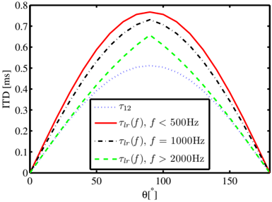
Fig. 1 : Comparison of τ 12 and τ lr ( f ) versus the angle of the desired sound for different frequencies.
<details>
<summary>Image 1 Details</summary>
### Visual Description
\n
## Chart: Interaural Time Difference (ITD) vs. Angle
### Overview
The image presents a chart illustrating the relationship between Interaural Time Difference (ITD) in milliseconds (ms) and angle θ̂ in degrees. Three curves are plotted, each representing a different frequency (f) range. The chart aims to demonstrate how ITD changes with angle for varying frequencies.
### Components/Axes
* **X-axis:** θ̂ [degrees]. Scale ranges from 0 to 180, with tick marks at 0, 50, 100, 150.
* **Y-axis:** ITD [ms]. Scale ranges from 0 to 0.8, with tick marks at 0, 0.2, 0.4, 0.6, 0.8.
* **Legend:** Located in the top-right corner. Contains the following entries:
* τ₁₂ (dotted line, grey)
* τIr(f), f < 500Hz (solid red line)
* τIr(f), f = 1000Hz (dashed black line)
* τIr(f), f > 2000Hz (dashed green line)
### Detailed Analysis
* **τIr(f), f < 500Hz (Red Line):** This curve exhibits a symmetrical, bell-shaped trend. It starts at approximately 0 ms at θ̂ = 0 degrees, rises to a peak of approximately 0.74 ms at θ̂ = 100 degrees, and then descends back to approximately 0 ms at θ̂ = 180 degrees.
* **τIr(f), f = 1000Hz (Black Dashed Line):** This curve also shows a symmetrical, bell-shaped trend, but with a higher peak and a narrower width compared to the red line. It starts at approximately 0 ms at θ̂ = 0 degrees, reaches a peak of approximately 0.78 ms at θ̂ = 100 degrees, and returns to approximately 0 ms at θ̂ = 180 degrees.
* **τIr(f), f > 2000Hz (Green Dashed Line):** This curve displays a similar symmetrical, bell-shaped trend, but with the lowest peak and narrowest width. It begins at approximately 0 ms at θ̂ = 0 degrees, peaks at approximately 0.65 ms at θ̂ = 100 degrees, and descends to approximately 0 ms at θ̂ = 180 degrees.
* **τ₁₂ (Grey Dotted Line):** This curve is a low amplitude, symmetrical curve. It starts at approximately 0.25 ms at θ̂ = 0 degrees, rises to a peak of approximately 0.32 ms at θ̂ = 100 degrees, and then descends back to approximately 0.25 ms at θ̂ = 180 degrees.
### Key Observations
* The ITD increases with angle up to a certain point (around 100 degrees) and then decreases.
* The peak ITD value decreases as the frequency increases. This suggests that higher frequencies have a smaller interaural time difference for a given angle.
* The width of the curves decreases as the frequency increases, indicating that the ITD is more sensitive to angle changes at higher frequencies.
* The τ₁₂ curve is consistently lower in magnitude than the other curves.
### Interpretation
The chart demonstrates the frequency-dependent nature of the Interaural Time Difference (ITD). ITD is a crucial cue for sound localization, particularly for low-frequency sounds. The data suggests that as frequency increases, the ITD becomes smaller and more sensitive to changes in angle. This is because higher frequencies have shorter wavelengths and are more easily diffracted around the head, reducing the time difference between when the sound reaches each ear. The τ₁₂ curve likely represents a baseline or reference value, potentially related to the head size or a constant delay. The relationship between ITD and frequency is fundamental to understanding how humans and other animals perceive the direction of sound. The curves are symmetrical, indicating that the ITD is independent of the direction of the sound source (left or right).
</details>
Kuhn has shown that the ITD is frequency-dependent [16], which can be approximately summarized as
<!-- formula-not-decoded -->
and, for f ≥ f H = 2000 ,
<!-- formula-not-decoded -->
where (9) and (10) are identical to [16, (7) and (12)], respectively. However, for the middle frequency range, there is not an explicit expression. We propose to use a linear interpolation to model the ITD in the middle frequency range, which agrees well with the measurement results [16] and is given by
<!-- formula-not-decoded -->
where f = f Mid ∈ [500 2000] Hz.
Compared to τ 12 , the ITD τ lr ( f ) is not only a function of the DOA but also of the frequency. τ 12 and τ lr ( f ) versus θ are plotted in Fig. 1 for different frequencies. Fig. 1 shows that the difference between | τ lr ( f ) | and | τ 12 | is largest for f ≤ 500 Hz. For f > 2000 Hz, τ lr ( f ) is close to τ 12 when | θ | or | π ± θ | is smaller than π/ 4 , while | τ lr ( f ) | is much larger than | τ 12 | for | θ | close to π/ 2 .
Without the shadowing effect of the head, the free-field coherence model of the desired signal is given by (3). Based on the frequency-dependent ITD model which accounts for the head effect, we can now define the coherence of the desired component for the binaural case as:
<!-- formula-not-decoded -->
## 3.2. Diffuse Noise Coherence Model
The shadowing effect of the head also has an impact on the spatial coherence of the two microphone signals in a diffuse
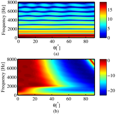
Fig. 2 : CDR estimation error of the free-field estimator, ∆ , versus f and θ for (a) the input CDR η in = -20 dB, (b) the input CDR η in = 20 dB.
<details>
<summary>Image 2 Details</summary>
### Visual Description
\n
## Heatmap: Frequency vs. Angle
### Overview
The image presents two heatmaps, labeled (a) and (b), displaying a relationship between frequency (in Hertz) and angle (in degrees). Both heatmaps share the same axes scales, but differ in the color scale and the distribution of values. The heatmaps appear to represent some form of spectral analysis or signal processing data.
### Components/Axes
* **X-axis:** θ [°] (Angle in degrees), ranging from 0 to 90.
* **Y-axis:** Frequency [Hz] (Frequency in Hertz), ranging from 0 to 8000.
* **Heatmap (a):** Color scale ranges from 0 to 15, with blue representing lower values and red representing higher values.
* **Heatmap (b):** Color scale ranges from -20 to 0, with blue representing higher values and red representing lower values.
* **Labels:** "(a)" and "(b)" identify the two heatmaps.
### Detailed Analysis or Content Details
**Heatmap (a):**
The heatmap shows roughly horizontal bands of color, indicating that the value is relatively constant for a given frequency but changes with angle.
* **0-1000 Hz:** Values are consistently low, around 0-2, appearing as dark blue.
* **1000-3000 Hz:** Values increase to approximately 5-8, appearing as yellow-green.
* **3000-6000 Hz:** Values are around 8-12, appearing as yellow-orange.
* **6000-8000 Hz:** Values are around 12-15, appearing as orange-red.
* There are slight variations in color intensity within each band, suggesting some angle-dependent fluctuations.
**Heatmap (b):**
This heatmap exhibits a more complex pattern. The color distribution is not banded like in (a).
* **0-20°:** Values are highly negative, around -15 to -20, appearing as dark red.
* **20-50°:** Values increase rapidly, transitioning from dark red to blue, reaching approximately 0 at around 50°.
* **50-80°:** Values remain around 0, with some fluctuations.
* **80-90°:** Values decrease again, becoming slightly negative, appearing as light red.
* There is a clear diagonal trend, with negative values at low angles and positive values at higher angles.
### Key Observations
* Heatmap (a) shows a frequency-dependent value that is relatively independent of the angle.
* Heatmap (b) shows a strong angle-dependent value, with a clear transition from negative to positive values as the angle increases.
* The color scales are different, indicating that the two heatmaps represent different quantities or have been normalized differently.
* The patterns in both heatmaps are smooth and continuous, suggesting that the underlying data is well-behaved.
### Interpretation
The two heatmaps likely represent different aspects of the same phenomenon. Heatmap (a) could represent the magnitude of a signal at different frequencies and angles, while heatmap (b) could represent the phase or some other property of the signal. The strong angle dependence in heatmap (b) suggests that the signal is sensitive to the angle of incidence or observation.
The transition from negative to positive values in heatmap (b) could indicate a change in the sign of the signal or a resonance effect. The specific meaning of the data would depend on the context of the experiment or simulation from which it was obtained.
The difference in color scales suggests that the two quantities are measured in different units or have different ranges. It is possible that one quantity is a logarithmic scale, while the other is a linear scale.
Without further information about the experiment or simulation, it is difficult to draw more specific conclusions about the data. However, the heatmaps provide valuable insights into the relationship between frequency, angle, and the measured quantity.
</details>
sound field. Both theoretical results and experimental results can be found in [17, 18]. Here we use the analytic representation of the binaural correlation function proposed by Lindevald and Benade [17], given by
<!-- formula-not-decoded -->
where α = 2 . 2 and β = 0 . 5 .
The binaural CDR estimators are now obtained by inserting the binaural coherence models Γ Binaural coh and Γ Binaural diff into the estimators given in Table 1. This extension makes the direction-dependent CDR estimators suitable for binaural dereverberation. The corresponding estimators are denoted as ˜ η Binaural · in the following, where · represents the name of the technique that is being used.
## 3.3. Robustness of the Free-Field Estimators in the Binaural Scenario
This part evaluates the robustness of the direction-dependent CDR estimators using the free-field model against the shadowing effect of the head. For the limited space of this paper, only ˜ η Binaural Schwarz2 is chosen to compare with ˜ η FF Schwarz2 , since a previous study [12] has already shown that ˜ η FF Schwarz2 has the best performance among the direction-dependent CDR estimators in Table 1 (see [12, Table III] for details). For the comparison, we generate values of the mixture coherence ˆ Γ x for a certain input CDR η in and different angles and frequencies according to the binaural coherence models defined above, and insert these coherence values into the free-field estimator. We then define the estimation error of the free-field CDR
Table 2 : PESQ scores averaged over all angles for CDR estimators in Table 1, using free-field ( ˜ η FF · ) or binaural coherence models ( ˜ η Binaural · ).
| AIR | Unprocessed | Direction-dependent | Direction-dependent | Direction-dependent | Direction-dependent | Direction-independent | Direction-independent | Direction-independent | Direction-independent |
|----------|---------------|-----------------------|-----------------------|-----------------------|-----------------------|-------------------------|-------------------------|-------------------------|-------------------------|
| Distance | Left/Right | ˜ η FF Schwarz1 | ˜ η Binaural Schwarz1 | ˜ η FF Schwarz2 | ˜ η Binaural Schwarz2 | ˜ η FF Thiergart2 | ˜ η Binaural Thiergart2 | ˜ η FF Schwarz3 | ˜ η Binaural Schwarz3 |
| 1m | 2.24/2.25 | 2.40/2.41 | 2.65/2.68 | 2.57/2.59 | 2.69/2.71 | 2.66/2.67 | 2.64/2.65 | 2.65/2.67 | 2.64/2.65 |
| 2m | 1.88/1.90 | 2.00/2.00 | 2.12/2.13 | 2.10/2.10 | 2.17/2.18 | 2.16/2.17 | 2.15/2.15 | 2.16/2.17 | 2.15/2.16 |
| 3m | 1.77/1.77 | 1.85/1.84 | 1.91/1.90 | 1.92/1.91 | 1.97/1.96 | 1.95/1.95 | 1.95/1.95 | 1.96/1.96 | 1.95/1.95 |
estimator compared to the true CDR η in as
<!-- formula-not-decoded -->
Fig. 2 plots ∆ versus f and θ for the true input CDR η in = -20 dB (a) and η in = 20 dB (b). Only θ ∈ [0 π/ 2] is considered due to the symmetry of the scenario. Fig. 2 shows that the CDR is somewhat overestimated for low input CDR, while for high input CDR, the CDR is seriously underestimated for angles larger than 45 ◦ . The influence of the head on the coherence, especially the one of the desired speech component Γ Binaural coh ( f ) , is significant enough to deteriorate the performance of the free-field CDR estimator considerably.
## 4. EVALUATION
This section evaluates the application of the CDR estimators in Table 1 with the free-field and binaural coherence models to the problem of dereverberation. We use the Aachen Impulse Response (AIR) database [19], which consists of binaural RIRs measured by a dummy head with azimuth angles from -90 ◦ to 90 ◦ with 15 ◦ increments and source-head distances from 1 m to 3 m with 1 m increments.
Ten clean speech samples (five female and five male speakers) are taken from the TIMIT database [20]. The reverberant speech samples are generated by convolving the clean speech with the 'stairway' RIRs from the AIR database. We use the same filterbank, postfilter gain function and parameters as in [12, (29)], with the CDR estimators in Table 1. Knowledge of the true DOA is assumed for computation of the desired signal coherence models. The gain function is applied to the two microphone signals separately. PESQ is chosen as evaluation measure since it was found to be highly correlated with speech quality for the evaluation of noise and reverberation suppression methods [21, 22]. Here, we give raw MOS scores obtained by wideband PESQ. The PESQ scores of the two microphone signals and those of the processed signals are given separately. Note that the average PESQ scores for both ears are very similar, due to the symmetry of the scenario. The experimental results for the different distances are presented in Table 2. From these results, we can make the following observations:
- (1) Using the ITD and binaural diffuse coherence model can improve all of the direction-dependent CDR estimators.
- (2) The direction-independent CDR estimators, which do not rely on a model of the desired signal coherence, are robust
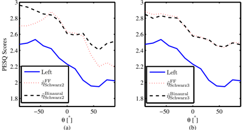
Fig. 3 : PESQ scores versus DOA for the 1 m distance case: (a) direction-dependent CDR estimators; (b) direction-independent CDR estimators. Left represents the unprocessed signal recorded by the microphone located at the left ear.
<details>
<summary>Image 3 Details</summary>
### Visual Description
\n
## Chart: PESQ Scores vs. Angle
### Overview
The image presents two line graphs (labeled (a) and (b)) displaying PESQ scores as a function of angle θ (in degrees). Each graph compares the PESQ scores for "FF ηSchwarz2" and "Binaural ηSchwarz2" (in graph (a)) and "FF ηSchwarz3" and "Binaural ηSchwarz3" (in graph (b)). The graphs appear to be evaluating the perceptual quality of audio signals under different spatial conditions.
### Components/Axes
* **X-axis:** θ [°] (Angle in degrees), ranging from approximately -60 to +60.
* **Y-axis:** PESQ Scores, ranging from approximately 1.8 to 3.0.
* **Legend (Graph a):**
* Blue Solid Line: Left - FF ηSchwarz2
* Black Dashed Line: Binaural ηSchwarz2
* **Legend (Graph b):**
* Red Dotted Line: FF ηSchwarz3
* Black Dashed Line: Binaural ηSchwarz3
* **Labels:** (a) and (b) identify the two separate graphs.
### Detailed Analysis or Content Details
**Graph (a):**
* **FF ηSchwarz2 (Blue Solid Line):** The line generally slopes downward from approximately -60° to 0°, reaching a minimum around 0° (approximately 2.1 PESQ score). It then increases slightly from 0° to +60°.
* At -60°: PESQ ≈ 2.55
* At -30°: PESQ ≈ 2.45
* At 0°: PESQ ≈ 2.1
* At +30°: PESQ ≈ 2.15
* At +60°: PESQ ≈ 2.2
* **Binaural ηSchwarz2 (Black Dashed Line):** This line exhibits a more pronounced peak around -30° (approximately 2.8 PESQ score) and a trough around 0° (approximately 1.9 PESQ score). It generally decreases from -60° to 0° and increases from 0° to +60°.
* At -60°: PESQ ≈ 2.7
* At -30°: PESQ ≈ 2.8
* At 0°: PESQ ≈ 1.9
* At +30°: PESQ ≈ 2.4
* At +60°: PESQ ≈ 2.5
**Graph (b):**
* **FF ηSchwarz3 (Red Dotted Line):** The line shows a peak around -30° (approximately 2.85 PESQ score) and a relatively flat trend around 0° (approximately 2.5 PESQ score). It decreases slightly from -30° to 0° and increases from 0° to +60°.
* At -60°: PESQ ≈ 2.7
* At -30°: PESQ ≈ 2.85
* At 0°: PESQ ≈ 2.5
* At +30°: PESQ ≈ 2.55
* At +60°: PESQ ≈ 2.6
* **Binaural ηSchwarz3 (Black Dashed Line):** This line is similar in shape to the Binaural line in graph (a), with a peak around -30° (approximately 2.7 PESQ score) and a trough around 0° (approximately 1.8 PESQ score).
* At -60°: PESQ ≈ 2.6
* At -30°: PESQ ≈ 2.7
* At 0°: PESQ ≈ 1.8
* At +30°: PESQ ≈ 2.3
* At +60°: PESQ ≈ 2.4
### Key Observations
* In both graphs, the "Binaural" lines consistently have lower PESQ scores around 0° compared to the "FF" lines.
* The "Binaural" lines exhibit more significant fluctuations in PESQ scores across the angle range than the "FF" lines.
* The "FF" lines are relatively stable across the angle range, with minor variations.
* Graph (b) shows a slight shift in the peak PESQ score for the "FF" line compared to graph (a).
* The "Binaural" lines in both graphs show a clear minimum around 0 degrees.
### Interpretation
These graphs likely represent the results of a perceptual audio quality evaluation. PESQ (Perceptual Evaluation of Speech Quality) is an objective metric that attempts to predict the perceived quality of speech after transmission or processing. The angle θ likely represents the spatial orientation of the sound source or the listener's head relative to the sound source.
The data suggests that the "FF" (presumably a front-facing or fixed-direction audio processing technique) provides more consistent audio quality across different spatial angles. The "Binaural" processing technique, while potentially offering higher quality in certain spatial configurations (around -30°), is more sensitive to the angle and experiences a significant drop in perceived quality when the sound source is directly in front (0°).
The difference between graphs (a) and (b) (using ηSchwarz2 vs. ηSchwarz3) indicates that the specific parameters or algorithms used in the binaural processing have a noticeable impact on the resulting PESQ scores. The consistent dip in the Binaural lines around 0° suggests a potential issue with the binaural rendering at that specific angle, possibly related to head-related transfer function (HRTF) inaccuracies or limitations. The data highlights the trade-offs between spatial audio processing techniques and the importance of considering the intended listening environment and spatial characteristics.
</details>
in the binaural case, even when using the free-field diffuse coherence model. This indicates that the choice of the diffuse coherence model is not critical, and the main effect of the head is on the ITD.
- (3) The direction-independent estimators almost reach the performance of the best binaural direction-dependent estimator.
To reveal the mechanism of the better performance of the proposed direction-dependent binaural CDR estimators, the PESQ scores versus θ are plotted in Fig. 3 (due to symmetry, only PESQ scores for the left microphone are shown). As can be seen from this figure, ˜ η Binaural Schwarz2 is much better than ˜ η FF Schwarz2 for | θ | ≥ 45 ◦ . This phenomenon can be explained by the robustness analysis results in Fig. 2, where it was found that the estimation error of ˜ η FF Schwarz2 becomes significant for | θ | > 45 ◦ . However, ˜ η FF Schwarz3 and ˜ η Binaural Schwarz3 nearly have the same performance for all angles, which confirms that the effect of using Γ FF diff ( f ) or Γ Binaural diff ( f ) is not critical for the direction-independent CDR estimators.
The estimators ˜ η Thiergart2 and ˜ η Schwarz3 show similar behavior in this scenario, although the former is biased [12]. This can be explained by the fact that the bias is roughly proportional to the noise coherence and disappears for Γ diff → 0 ; since, for binaural signals, the noise coherence is lower than for the setup investigated in [12], due to the large spacing of the sensors and the shadowing effect of the head, the practical impact of the bias is not significant here.
## 5. CONCLUSIONS
This paper extends previously proposed free-field CDR estimators to binaural dereverberation by using a simplified model for the ITD. Experimental results show that this extension is important for the direction-dependent CDR estimators, where PESQ scores for dereverberation can be significantly improved. It is further shown that the direction-independent CDR estimators, which do not require a model of the desired signal coherence, can achieve similar performance and are robust towards the shadowing effect of the head. Further work could concentrate on studying the impact of the ILD on binaural dereverberation and the theoretical limits of the CDR estimators by using statistical analysis [23].
## REFERENCES
- [1] M. Brandstein, and D. Ward, Microphone arrays: signal processing techniques and applications . Berlin: Springer-Verlag, 2001.
- [2] J. Benesty, S. Makino, and J. Chen, Speech Enhancement . Berlin: Springer-Verlag, 2005.
- [3] P. A. Naylor, and N. D. Gaubitch, Speech dereverberation . London: Springer-Verlag, 2010.
- [4] J. B. Allen, D. A. Berkley, and J. Blauert. 'Multimicrophone signal-processing technique to remove room reverberation from speech signals.' J. Acoust. Soc. Am. , vol. 62, pp. 912-915, 1977.
- [5] K. Lebart, J. Boucher, and P. Denbigh. 'A binaural system for the suppression of late reverberation.' in Proc. EUSIPCO , Island of Rhodes, Greece, 1998.
- [6] M. Jeub, M. Schafer, T. Esch, and P. Vary. 'Model-based dereverberation preserving binaural cues.' IEEE Trans. Audio, Speech, and Lang. Process. , vol. 18, pp. 17321745, 2010.
- [7] A. Kuklasinski, S. Doclo, S. H. Jensen, and J. Jensen. 'Maximum likelihood based multi-channel isotropic reverberation reduction for hearing aids.' in Proc. EUSIPCO , Lisbon, Portugal, 2014.
- [8] A. Westermann, J. M. Buchholz, and T. Dau. 'Binaural dereverberation based on interaural coherence histograms.' J. Acoust. Soc. Am. , vol. 133, pp. 2767-2777, 2013.
- [9] A. Tsilfidis, A.Westermann, J. M. Buchholz, E. Georganti and J. Mourjopoulos. Binaural Dereverberation . Berlin: Springer-Verlag, 2013.
- [10] V. Hamacher, J. Chalupper, J. Eggers, E. Fischer, U. Kornagel, H. Puder, U. Rass. 'Signal Processing in HighEnd Hearing Aids: State of the Art, Challenges, and Future Trends.' EURASIP J. on Adv. in Signal Process. , vol. 18, pp. 2915-2929, 2005.
- [11] O. Thiergart, G. Del Galdo, and E. A. P. Habets. 'Signal-to-reverberant ratio estimation based on the complex spatial coherence between omnidirectional microphones.' in Proc. ICASSP , Kyoto, Japan, 2012.
- [12] A. Schwarz, and W. Kellermann. 'Coherent-to-diffuse power ratio estimation for dereverberation.' IEEE/ACM Trans. on Audio, Speech and Lang. Process. , vol. 23, pp. 1006-1018, 2015.
- [13] J. Blauert. Spatial Hearing . The MIT Press: Harvard MA, 1997.
- [14] J. Blauert. The Technology of Binaural Listening . Berlin-Heidelberg-New York: Springer-Verlag, 2013.
- [15] T. Qu, Z. Xiao, M. Gong, Y. Huang, X. Li, and X. Wu. 'Distance-dependent head-related transfer functions measured with high spatial resolution using a spark gap.' IEEE Trans. on Audio, Speech, and Lang. Process. , vol. 17, no. 6, pp. 1124-1132, Aug. 2009.
- [16] G. F. Kuhn. 'Model for the interaural time differences in the azimuthal plane.' J. Acoust. Soc. Am. , vol. 62, pp. 157-167, 1977.
- [17] I. M. Lindevald and A. H. Benade. 'Two-ear correlation in the statistical sound fields of rooms.' J. Acoust. Soc. Am. , vol. 80, pp. 661-664, 1986.
- [18] M. Jeub, M. Dorbecker and P. Vary. 'A semi-analytical model for the binaural coherence of noise fields.' IEEE Signal Process. Letters , vol. 18, pp. 197-200, 2011.
- [19] M. Jeub, M. Schafer, and P. Vary. 'A binaural room impulse response database for the evaluation of dereverberation algorithms.' in Proc. Int. Conf. Digital Signal Process. (DSP) , Santorini, Greece, 2009.
- [20] J. S. Garofolo. 'Getting Started With the DARPA TIMIT CD-ROM: An Acoustic-Phonetic Continous Speech Database.' Nat. Inst. of Standards and Technology (NIST) , Gaithersburg, MD, 1993.
- [21] Y. Hu and P. C. Loizou. 'Evaluation of objective quality measures for speech enhancement.' IEEE Trans. Audio, Speech and Lang. Process. , vol. 16, pp. 229-238, 2008.
- [22] S. Goetze, A. Warzybok, I. Kodrasi, J. O. Jungmann, B. Cauchi, J. Rennies, E. A. P. Habets, A. Mertins, T. Gerkmann, S. Doclo, and B. Kollmeier. 'A Study on Speech Quality and Speech Intelligibility Measures for Quality Assessment of Single-Channel Dereverberation Algorithms,.' in Proc. IWAENC , Antibes, France, 2014.
- [23] C. Zheng, H. Liu, R. Peng,and X. Li. 'A Statistical Analysis of Two-Channel Post-Filter Estimators in Isotropic Noise Fields.' IEEE Trans. on Audio, Speech, and Lang. Process. , vol. 21, pp. 336-342, 2013.