1603.07704

## Probabilistic Reasoning via Deep Learning: Neural Association Models Quan Liu † , Hui Jiang ‡ , Andrew Evdokimov ‡ , Zhen-Hua Ling † , Xiaodan Zhu , Si Wei § , Yu Hu †§ † National Engineering Laboratory for Speech and Language Information Processing University of Science and Technology of China, Hefei, Anhui, China ‡ Department of Electrical Engineering and Computer Science, York University, Canada National Research Council Canada, Ottawa, Canada § iFLYTEK Research, Hefei, China emails: quanliu@mail.ustc.edu.cn, hj@cse.yorku.ca, ae2718@cse.yorku.ca, zhling@ustc.edu.cn xiaodan@cse.yorku.ca, siwei@iflytek.com, yuhu@iflytek.com ## Abstract In this paper, we propose a new deep learning approach, called neural association model (NAM), for probabilistic reasoning in artificial intelligence. We propose to use neural networks to model association between any two events in a domain. Neural networks take one event as input and compute a conditional probability of the other event to model how likely these two events are to be associated. The actual meaning of the conditional probabilities varies between applications and depends on how the models are trained. In this work, as two case studies, we have investigated two NAM structures, namely deep neural networks (DNN) and relation-modulated neural nets (RMNN), on several probabilistic reasoning tasks in AI, including recognizing textual entailment, triple classification in multi-relational knowledge bases and commonsense reasoning. Experimental results on several popular datasets derived from WordNet, FreeBase and ConceptNet have all demonstrated that both DNNs and RMNNs perform equally well and they can significantly outperform the conventional methods available for these reasoning tasks. Moreover, compared with DNNs, RMNNs are superior in knowledge transfer, where a pre-trained model can be quickly extended to an unseen relation after observing only a few training samples. To further prove the effectiveness of the proposed models, in this work, we have applied NAMs to solving challenging Winograd Schema (WS) problems. Experiments conducted on a set of WS problems prove that the proposed models have the potential for commonsense reasoning. ## Introduction Reasoning is an important topic in artificial intelligence (AI), which has attracted considerable attention and research effort in the past few decades (McCarthy 1986; Minsky 1988; Mueller 2014). Besides the traditional logic reasoning, probabilistic reasoning has been studied as another typical genre in order to handle knowledge uncertainty in reasoning based on probability theory (Pearl 1988; Neapolitan 2012). The probabilistic reasoning can be used to predict conditional probability Pr( E 2 | E 1 ) of one event E 2 given another event E 1 . State-of-the-art methods for probabilistic reasoning include Bayesian Networks (Jensen 1996), Markov Logic Networks (Richardson and Domingos 2006) and other graphical models (Koller and Friedman 2009). Taking Bayesian networks as an example, the conditional Copyright 2015-2016. probabilities between two associated events are calculated as posterior probabilities according to Bayes theorem, with all possible events being modeled by a pre-defined graph structure. However, these methods quickly become intractable for most practical tasks where the number of all possible events is usually very large. In recent years, distributed representations that map discrete language units into continuous vector space have gained significant popularity along with the development of neural networks (Bengio et al. 2003; Collobert et al. 2011; Mikolov et al. 2013). The main benefit of embedding in continuous space is its smoothness property, which helps to capture the semantic relatedness between discrete events, potentially generalizable to unseen events. Similar ideas, such as knowledge graph embedding, have been proposed to represent knowledge bases (KB) in low-dimensional continuous space (Bordes et al. 2013; Socher et al. 2013; Wang et al. 2014; Nickel et al. 2015). Using the smoothed KB representation, it is possible to reason over the relations among various entities. However, human-like reasoning remains as an extremely challenging problem partially because it requires the effective encoding of world knowledge using powerful models. Most of the existing KBs are quite sparse and even recently created large-scale KBs, such as YAGO, NELL and Freebase, can only capture a fraction of world knowledge. In order to take advantage of these sparse knowledge bases, the state-of-the-art approaches for knowledge graph embedding usually adopt simple linear models, such as RESCAL (Nickel, Tresp, and Kriegel 2012), TransE (Bordes et al. 2013) and Neural Tensor Networks (Socher et al. 2013; Bowman 2013). Although deep learning techniques achieve great progresses in many domains, e.g. speech and image (LeCun, Bengio, and Hinton 2015), the progress in commonsense reasoning seems to be slow. In this paper, we propose to use deep neural networks, called neural association model (NAM) , for commonsense reasoning. Different from the existing linear models, the proposed NAM model uses multilayer nonlinear activations in deep neural nets to model the association conditional probabilities between any two possible events. In the proposed NAM framework, all symbolic events are represented in low-dimensional continuous space and there is no need to explicitly specify any dependency structure among events as required in Bayesian networks. Deep neural networks are used to model the association between any two events, taking one event as input to compute a conditional probability of another event. The computed conditional probability for association may be generalized to model various reasoning problems, such as entailment inference, relational learning, causation modelling and so on. In this work, we study two model structures for NAM. The first model is a standard deep neural networks (DNN) and the second model uses a special structure called relation modulated neural nets (RMNN). Experiments on several probabilistic reasoning tasks, including recognizing textual entailment, triple classification in multi-relational KBs and commonsense reasoning, have demonstrated that both DNNs and RMNNs can outperform other conventional methods. Moreover, the RMNN model is shown to be effective in knowledge transfer learning, where a pre-trained model can be quickly extended to a new relation after observing only a few training samples. Furthermore, we also apply the proposed NAM models to more challenging commonsense reasoning problems, i.e., the recently proposed Winograd Schemas (WS) (Levesque, Davis, and Morgenstern 2011). The WS problems has been viewed as an alternative to the Turing Test (Turing 1950). To support the model training for NAM, we propose a straightforward method to collect associated cause-effect pairs from large unstructured texts. The pair extraction procedure starts from constructing a vocabulary with thousands of common verbs and adjectives. Based on the extracted pairs, this paper extends the NAM models to solve the Winograd Schema problems and achieves a 61% accuracy on a set of causeeffect examples. Undoubtedly, to realize commonsense reasoning, there is still much work be done and many problems to be solved. Detailed discussions would be given at the end of this paper. ## Motivation: Association between Events This paper aims to model the association relationships between events using neural network methods. To make clear our main work, we will first describe the characteristics of events and all the possible association relationships between events. Based on the analysis of event association, we present the motivation for the proposed neural association models. In commonsense reasoning, the main characteristics of events are the following: - Massive : In most natural situations, the number of events is massive, which means that the association space we will model is very large. - Sparse : All the events occur in our dialy life are very sparse. It is a very challenging task to ideally capture the similarities between all those different events. 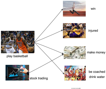At the same time, association between events appears everywhere. Consider a single event play basketball for example, shown in Figure 1. This single event would associate with many other events. A person who plays basketball would win a game. Meanwhile, he would be injured in some cases. The person could make money by playing basketball as well. Moreover, we know that a person who plays basketball should be coached during a regular game. Those are all typical associations between events. However, we need to recognize that the task of modeling event association is not identical to performing classification . In classification, we typically map an event from its feature space into one of pre-defined finite categories or classes. In event association, we need to compute the association probability between two arbitrary events, each of which may be a sample from a possibly infinite set. The mapping relationships in event association would be many-to-many ; e.g., not only playing basketball could support us to make money, someone who makes stock trading could make money as well. More specifically, the association relationships between events include causeeffect, spatial, temporal and so on. This paper treats them as a general relation considering the sparseness of useful KBs. Figure 1: Example of association between events. <details> <summary>Image 1 Details</summary>  ### Visual Description ## Diagram: Basketball-Related Activities and Outcomes ### Overview The diagram illustrates a central node labeled "play basketball" connected via arrows to six secondary nodes, each representing distinct outcomes or related activities. The structure suggests a causal or associative relationship between playing basketball and the listed outcomes, with "stock trading" acting as a secondary node that further branches into "be coached" and "drink water." ### Components/Axes - **Central Node**: "play basketball" (labeled in black text, positioned at the center-left of the diagram). - **Direct Connections**: - "win" (top-right, image of a runner). - "injured" (middle-right, image of a person on the ground). - "make money" (bottom-right, image of cash). - "stock trading" (bottom-left, image of a hand interacting with a stock chart). - **Secondary Connections from "stock trading"**: - "be coached" (bottom-center, image of a group of people). - "drink water" (bottom-right, image of a person drinking water). ### Detailed Analysis - **Node Relationships**: - "play basketball" directly connects to "win," "injured," "make money," and "stock trading." - "stock trading" has two outgoing arrows to "be coached" and "drink water," indicating a secondary relationship. - **Visual Elements**: - Each node includes an image that visually represents the label (e.g., cash for "make money," a stock chart for "stock trading"). - Arrows are black, with no labels, implying directional flow from the central node to the outcomes. ### Key Observations - The diagram emphasizes the multifaceted nature of playing basketball, linking it to both positive (win, make money) and negative (injured) outcomes. - "Stock trading" is positioned as a distinct but related activity, with its own sub-branches ("be coached," "drink water"), suggesting it may require additional resources or conditions. - No numerical data or quantitative values are present; the diagram focuses on conceptual relationships. ### Interpretation The diagram appears to map the potential consequences, opportunities, and ancillary activities associated with playing basketball. The inclusion of "stock trading" as a secondary node implies a possible overlap between athletic pursuits and financial activities, though the exact nature of this relationship is not explicitly defined. The sub-branches from "stock trading" ("be coached," "drink water") may metaphorically highlight the need for guidance and self-care in high-pressure environments, though this interpretation is speculative without additional context. The lack of numerical data limits quantitative analysis, but the structure emphasizes interconnectedness between physical activity and broader life outcomes. </details> In this paper, we believe that modeling the the association relationships between events is a fundamental work for commonsense reasoning. If we could model the event associations very well, we may have the ability to solve many commonsense reasoning problems. Considering the main characteristics of discrete event and event association , two reasons are given for describing our motivation. - The advantage of distributed representation methods: representing discrete events into continuous vector space provides a good way to capture the similarities between discrete events. - The advantage of neural network methods: neural networks could perform universal approximation while linear models cannot easily do this (Hornik, Stinchcombe, and White 1990). At the same time, this paper takes into account that both distributed representation and neural network methods are data-hungry. In Artificial Intelligence (AI) research, mining large sizes of useful data (or knowledge) for model learning is always challenging. In the following section, this paper presents a preliminary work on data collection and the corresponding experiments we have made for solving commonsense reasoning problems. 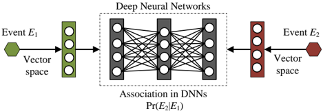## Neural Association Models (NAM) In this paper, we propose to use a nonlinear model, namely neural association model, for probabilistic reasoning. Our main goal is to use neural nets to model the association probability for any two events E 1 and E 2 in a domain, i.e., Pr( E 2 | E 1 ) of E 2 conditioning on E 1 . All possible events in the domain are projected into continuous space without specifying any explicit dependency structure among them. In the following, we first introduce neural association models (NAM) as a general modeling framework for probabilistic reasoning. Next, we describe two particular NAM structures for modeling the typical multi-relational data. ## NAMin general Figure 2: The NAM framework in general. <details> <summary>Image 2 Details</summary>  ### Visual Description ## Diagram: Deep Neural Network Event Association ### Overview The diagram illustrates the process of event association in deep neural networks (DNNs), showing how input events (E₁) are transformed into output events (E₂) through vector space encoding and neural network processing. The flow is directional, with clear input-output relationships and probabilistic associations. ### Components/Axes 1. **Left Side (Input):** - **Event E₁**: Represented by a green hexagon labeled "Event E₁" - **Vector Space**: Green vertical rectangle with 4 white circles (nodes) labeled "Vector space" - **Flow**: Black arrow from E₁ to vector space 2. **Center (Processing):** - **Deep Neural Networks**: Gray box containing 3 dense layers of interconnected nodes (circles with black lines) - **Association Label**: Bottom of DNN box shows "Association in DNNs" with probability notation "Pr(E₂|E₁)" 3. **Right Side (Output):** - **Vector Space**: Red vertical rectangle with 4 white circles labeled "Vector space" - **Event E₂**: Red hexagon labeled "Event E₂" - **Flow**: Black arrow from vector space to E₂ 4. **Legend:** - Green hexagon = Event E₁ - Red hexagon = Event E₂ - Positioned at top-left of diagram ### Detailed Analysis - **Input Encoding**: Event E₁ is first converted into a 4-dimensional vector representation (4 nodes in green vector space) - **Neural Network Architecture**: - 3 dense layers with full interconnections (each node in layer connected to all nodes in adjacent layers) - Total nodes: 4 (input) + 8 (hidden) + 8 (hidden) + 4 (output) = 24 nodes - **Output Decoding**: Processed vector space (4 nodes in red) is converted back to Event E₂ representation - **Probabilistic Association**: Explicitly labeled as conditional probability Pr(E₂|E₁) indicating learned dependency between events ### Key Observations 1. Symmetrical vector space representations for both input and output events 2. Consistent node count (4 nodes) in both input and output vector spaces 3. Dense layer configuration follows standard DNN architecture patterns 4. Explicit probabilistic notation grounds the association in statistical terms ### Interpretation This diagram demonstrates how DNNs learn temporal or causal relationships between events through: 1. **Feature Encoding**: Converting raw events into vector representations 2. **Non-linear Transformation**: Through multiple dense layers capturing complex patterns 3. **Probabilistic Output**: Modeling event dependencies as conditional probabilities The symmetrical architecture suggests the network learns bidirectional relationships between events, though the directional flow emphasizes E₁→E₂ prediction. The use of vector spaces implies dimensionality reduction/feature extraction capabilities, while the dense layers enable capture of intricate event associations. The explicit probability notation grounds the model's output in statistical inference rather than deterministic mapping. </details> Figure 2 shows the general framework of NAM for associating two events, E 1 and E 2 . In the general NAM framework, the events are first projected into a low-dimension continuous space. Deep neural networks with multi-layer nonlinearity are used to model how likely these two events are to be associated. Neural networks take the embedding of one event E 1 (antecedent) as input and compute a conditional probability Pr( E 2 | E 1 ) of the other event E 2 (consequent). If the event E 2 is binary (true or false), the NAM models may use a sigmoid node to compute Pr( E 2 | E 1 ) . If E 2 takes multiple mutually exclusive values, we use a few softmax nodes for Pr( E 2 | E 1 ) , where it may need to use multiple embeddings for E 2 (one per value). NAMs do not explicitly specify how different events E 2 are actually related; they may be mutually exclusive, contained, intersected. NAMs are only used to separately compute conditional probabilities, Pr( E 2 | E 1 ) , for each pair of events, E 1 and E 2 , in a task. The actual physical meaning of the conditional probabilities Pr( E 2 | E 1 ) varies between applications and depends on how the models are trained. Table 1 lists a few possible applications. Table 1: Some applications for NAMs. | Application | E 1 | E 2 | |------------------------------------|---------------|-------------| | language modeling causal reasoning | h | w e j W 2 D | | | cause | effect | | knowledge triple classification | { e i , r k } | | | lexical entailment | W 1 | | | textual entailment | D 1 | 2 | In language modeling, the antecedent event is the representation of historical context, h , and the consequent event is the next word w that takes one out of K values. In causal reasoning, E 1 and E 2 represent cause and effect respectively. For example, we have E 1 = 'eating cheesy cakes' and E 2 = 'being happy' , where Pr( E 2 | E 1 ) indicates how likely it is that E 1 may cause the binary (true or false) event E 2 . In the same model, we may add more nodes to model different effects from the same E 1 , e.g., E ′ 2 = 'growing fat' . Moreover, we may add 5 softmax nodes to model a multi-valued event, e.g., E ′′ 2 = 'happiness' (scale from 1 to 5) . Similarly, for knowledge triple classification of multi-relation data, given one triple ( e i , r k , e j ) , E 1 consists of the head entity ( subject ) e i and relation ( predicate ) r k , and E 2 is a binary event indicating whether the tail entity ( object ) e j is true or false. Finally, in the applications of recognizing lexical or textual entailment, E 1 and E 2 may be defined as premise and hypothesis . More generally, NAMs can be used to model an infinite number of events E 2 , where each point in a continuous space represents a possible event. In this work, for simplicity, we only consider NAMs for a finite number of binary events E 2 but the formulation can be easily extended to more general cases. Compared with traditional methods, like Bayesian networks, NAMs employ neural nets as a universal approximator to directly model individual pairwise event association probabilities without relying on explicit dependency structure. Therefore, NAMs can be end-to-end learned purely from training samples without strong human prior knowledge, and are potentially more scalable to real-world tasks. Learning NAMs Assume we have a set of N d observed examples (event pairs { E 1 , E 2 } ), D , each of which is denoted as x n . This training set normally includes both positive and negative samples. We denote all positive samples ( E 2 = true ) as D + and all negative samples ( E 2 = false ) as D -. Under the same independence assumption as in statistical relational learning (SRL) (Getoor 2007; Nickel et al. 2015), the log likelihood function of a NAM model can be expressed as follows: $$\mathcal { L } ( \Theta ) = \sum _ { x _ { n } ^ { + } \in \mathcal { D } ^ { + } } \ln f ( x _ { n } ^ { + } ; \Theta ) + \sum _ { x _ { n } ^ { - } \in \mathcal { D } ^ { - } } \ln ( 1 - f ( x _ { n } ^ { - } ; \Theta ) )$$ where f ( x n ; Θ ) denotes a logistic score function derived by the NAM for each x n , which numerically computes the conditional probability Pr( E 2 | E 1 ) . More details on f ( · ) will be given later in the paper. Stochastic gradient descent (SGD) methods may be used to maximize the above likelihood function, leading to a maximum likelihood estimation (MLE) for NAMs. In the following, as two case studies, we consider two NAM structures with a finite number of output nodes to model Pr( E 2 | E 1 ) for any pair of events, where we have only a finite number of E 2 and each E 2 is binary. The first model is a typical DNN that associates antecedent event ( E 1 ) at input and consequent event ( E 2 ) at output. We then present another model structure, called relation-modulated neural nets, which is more suitable for multi-relational data. 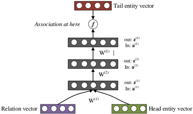xisted Relations ( L ) …… (2) (1) (head) ector Event Vector space E Head entity vector Tail entity vector ## DNN for NAMs Event E Head entity vector Event E The first NAM structure is a traditional DNN as shown in Figure 3. Here we use multi-relational data in KB for illustration. Given a KB triple x n = ( e i , r k , e j ) and its corresponding label y n (true or false), we cast E 1 = ( e i , r k ) and E 2 = e j to compute Pr( E 2 | E 1 ) as follows. Vector space Vector space Association in DNNs P( E 2 | E 1 ) <details> <summary>Image 3 Details</summary>  ### Visual Description ## Neural Network Architecture Diagram: Entity-Relation Association Model ### Overview The diagram illustrates a multi-layer neural network architecture for modeling associations between entities and relations. It shows the flow of information from input vectors (head entity, tail entity, and relation) through multiple transformation layers to output association vectors. The architecture includes explicit weight matrices and a final association function. ### Components/Axes 1. **Input Vectors**: - **Head entity vector** (green block): Positioned at the bottom-right - **Tail entity vector** (red block): Positioned at the top - **Relation vector** (purple block): Positioned at the bottom-left 2. **Transformation Layers**: - Three stacked layers labeled W^(1), W^(2), ..., W^(L) - Each layer has: - Input vector (z^(i)) - Output vector (a^(i)) - Weight matrix (W^(i)) connecting input to output 3. **Association Function**: - Labeled "f" at the top of the architecture - Connects final output vector (a^(L)) to the tail entity vector 4. **Output Vectors**: - Sequence of z^(1) to z^(L) vectors - Sequence of a^(1) to a^(L) vectors ### Detailed Analysis - **Input Flow**: - Head entity vector (W^(1)) and relation vector (W^(1)) combine at the first layer - Tail entity vector connects directly to the top of the architecture - **Layer Progression**: - Each layer transforms input vectors through weight matrices - Output of layer i becomes input for layer i+1 - Final layer output (a^(L)) connects to the tail entity vector via function f - **Vector Relationships**: - z^(i) represents intermediate feature representations - a^(i) represents association strength at each layer - Final a^(L) determines the association strength between head and tail entities ### Key Observations 1. The architecture uses a bottom-up approach, starting with raw entity/relation vectors 2. Multiple transformation layers suggest hierarchical feature learning 3. The association function f appears to be a non-linear combination of the final layer output 4. No explicit activation functions are shown between layers 5. All vectors maintain consistent dimensionality through the network ### Interpretation This architecture demonstrates a compositional model for entity-relation association: 1. **Feature Composition**: The relation vector combines with head entity features in the first layer 2. **Progressive Refinement**: Each subsequent layer refines the association representation 3. **Tail Entity Integration**: The final association strength directly influences the tail entity vector 4. **Interpretability**: The layered structure allows tracing association strength through intermediate representations The model likely implements a form of neural tensor network or relation network, where: - W^(1) learns initial relation-aware features - Deeper layers (W^(2)...W^(L)) capture complex interaction patterns - The final association function f could represent a sigmoid or softmax for probability prediction This structure enables the network to model complex semantic relationships between entities while maintaining interpretability through its explicit weight matrices and association function. </details> V (head) Tail entity vector Figure 3: The DNN structure for NAMs. Tail entity vector f Association at here W (2) W ( L ) … out: z ( L ) In: a ( L ) out: z (2) In: a (2) … B (2) B ( L ) B ( L+ 1) Firstly, we represent head entity phrase e i and tail entity phrase e j by two embedding vectors v (1) i ( ∈ V (1) ) and v (2) j ( ∈ V (2) ) . Similarly, relation r k is also represented by a low-dimensional vector c k ∈ C , which we call a relation code hereafter. Secondly, we combine the embeddings of the head entity e i and the relation r k to feed into an ( L + 1) -layer DNN as input. The DNN consists of L rectified linear (ReLU) hidden layers (Nair and Hinton 2010). The input is z (0) = [ v (1) i , c k ] . During the feedforward process, we have $$a ^ { ( \ell ) } = W ^ { ( \ell ) } z ^ { ( \ell - 1 ) } + b ^ { \ell } \quad ( \ell = 1 , \cdots , L ) \quad ( 2 )$$ W (1) $$z ^ { ( \ell ) } = h \left ( a ^ { ( \ell ) } \right ) = \max \left ( 0 , a ^ { ( \ell ) } \right ) \quad ( \ell = 1 , \cdots , L ) \quad ( 3 )$$ where W ( ) and b represent the weight matrix and bias for layer respectively. Finally, we propose to calculate a sigmoid score for each triple x n = ( e i , r k , e j ) as the association probability using the last hidden layer's output and the tail entity vector v (2) j : $$f ( x _ { n } ; \Theta ) = \sigma \left ( z ^ { ( L ) } \cdot v _ { j } ^ { ( 2 ) } \right ) \quad ( 4 )$$ -x where σ ( · ) is the sigmoid function, i.e., σ ( x ) = 1 / (1+ e ) . All network parameters of this NAM structure, represented as Θ = { W , V (1) , V (2) , C } , may be jointly learned by maximizing the likelihood function in eq. (1). 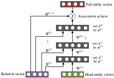## Relation-modulated Neural Networks (RMNN) Particularly for multi-relation data, following the idea in (Xue et al. 2014), we propose to use the so-called relationmodulated neural nets (RMNN), as shown in Figure 4. The RMNN uses the same operations as DNNs to project all entities and relations into low-dimensional continuous space. As shown in Figure 4, we connect the knowledgespecific relation code c ( k ) to all hidden layers in the network. New Relation Deep Neural Networks Tail entity vector Figure 4: The relation-modulated neural networks (RMNN). <details> <summary>Image 4 Details</summary>  ### Visual Description ## Diagram: Entity-Relation Association Architecture ### Overview The diagram illustrates a multi-layered neural network architecture for entity-relation association. It depicts the flow of information from a **Head entity vector** and **Relation vector** through sequential processing blocks to produce a **Tail entity vector**. The architecture includes multiple transformation layers (B and W) and a final association function (f). ### Components/Axes 1. **Key Elements**: - **Head entity vector**: Green block at the bottom-right. - **Relation vector**: Purple block at the bottom-left. - **Tail entity vector**: Red block at the top-right. - **Processing blocks**: - **B^(1) to B^(L+1)**: Vertical stack of gray blocks on the left, labeled with superscripts (B^(1), B^(2), ..., B^(L+1)). - **W^(1) to W^(L)**: Vertical stack of gray blocks in the center, labeled with superscripts (W^(1), W^(2), ..., W^(L)). - **Arrows**: Indicate directional flow (e.g., from Head entity vector to B^(1), then upward through B^(2) to B^(L+1)). - **Function "f"**: Connects B^(L+1) to the Tail entity vector, labeled "Association at here." 2. **Color Coding**: - **Green**: Head entity vector. - **Purple**: Relation vector. - **Red**: Tail entity vector. - **Gray**: Processing blocks (B and W). 3. **Textual Labels**: - Inputs: - Head entity vector: "In: a^(1)" (W^(1)), "In: a^(2)" (W^(2)), ..., "In: a^(L)" (W^(L)). - Outputs: - "out: z^(1)" (W^(1)), "out: z^(2)" (W^(2)), ..., "out: z^(L)" (W^(L)). - Function: "f" (association step). ### Detailed Analysis - **Flow Direction**: 1. The **Head entity vector** (green) and **Relation vector** (purple) are combined at B^(1). 2. The output of B^(1) is passed to W^(1), producing "out: z^(1)." 3. This process repeats iteratively: B^(i) processes inputs, W^(i) generates outputs, and the sequence progresses upward. 4. At the top layer (B^(L+1)), the output is fed into function "f," which generates the **Tail entity vector** (red). - **Component Relationships**: - The **B^(i)** blocks likely represent bidirectional or contextual transformation layers. - The **W^(i)** blocks appear to be weight matrices or linear transformations. - Function "f" acts as the final association mechanism, integrating all prior transformations. ### Key Observations - The architecture is hierarchical, with increasing complexity from B^(1) to B^(L+1). - The **Tail entity vector** depends on the cumulative output of all B and W layers. - No numerical values or quantitative data are present; the diagram focuses on structural relationships. ### Interpretation This diagram represents a **sequence-to-sequence model** or **transformer-like architecture** for entity-relation prediction. The Head and Tail entity vectors likely correspond to subject and object entities in a knowledge graph, while the Relation vector encodes their interaction. The layers B and W progressively refine the association, with "f" serving as the final classifier or regressor. The absence of numerical data suggests this is a conceptual blueprint rather than an empirical analysis. **Critical Insight**: The iterative processing of B and W layers implies a focus on capturing long-range dependencies, common in models like BERT or GPT for contextual understanding. The "association at here" label emphasizes the importance of the final function "f" in determining the Tail entity. </details> As shown later, this structure is superior in knowledge transfer learning tasks. Therefore, for each layer of RMNNs, instead of using eq.(2), its linear activation signal is computed from the previous layer z ( -1) and the relation code c ( k ) as follows: $$a ^ { ( \ell ) } = W ^ { ( \ell ) } z ^ { ( \ell - 1 ) } + B ^ { ( \ell ) } c ^ { ( k ) } , \quad ( \ell = 1 \cdots L ) \quad ( 5 )$$ where W ( ) and B represent the normal weight matrix and the relation-specific weight matrix for layer . At the topmost layer, we calculate the final score for each triple x n = ( e i , r k , e j ) using the relation code as: $$f ( x _ { n } ; \Theta ) = \sigma \left ( z ^ { ( L ) } \cdot v _ { j } ^ { ( 2 ) } + B ^ { ( L + 1 ) } \cdot c ^ { ( k ) } \right ) . \quad ( 6 )$$ In the same way, all RMNN parameters, including Θ = { W , B , V (1) , V (2) , C } , can be jointly learned based on the above maximum likelihood estimation. The RMNN models are particularly suitable for knowledge transfer learning , where a pre-trained model can be quickly extended to any new relation after observing a few samples from that relation. In this case, we may estimate a new relation code based on the available new samples while keeping the whole network unchanged. Due to its small size, the new relation code can be reliably estimated from only a small number of new samples. Furthermore, model performance in all original relations will not be affected since the model and all original relation codes are not changed during transfer learning. ## Experiments In this section, we evaluate the proposed NAM models for various reasoning tasks. We first describe the experimental setup and then we report the results from several reasoning tasks, including textual entailment recognition, triple classification in multi-relational KBs, commonsense reasoning and knowledge transfer learning. ## Experimental setup Here we first introduce some common experimental settings used for all experiments: 1) For entity or sentence representations, we represent them by composing from their word vectors as in (Socher et al. 2013). All word vectors are initialized from a pre-trained skip-gram (Mikolov et al. 2013) word embedding model, trained on a large English Wikipedia corpus. The dimensions for all word embeddings are set to 100 for all experiments; 2) The dimensions of all relation codes are set to 50. All relation codes are randomly initialized; 3) For network structures, we use ReLU as the nonlinear activation function and all network parameters are initialized according to (Glorot and Bengio 2010). Meanwhile, since the number of training examples for most probabilistic reasoning tasks is relatively small, we adopt the dropout approach (Hinton et al. 2012) during the training process to avoid the over-fitting problem; 4) During the learning process of NAMs, we need to use negative samples, which are automatically generated by randomly perturbing positive KB triples as D -= { ( e i , r k , e ) | e = e j ∧ ( e i , r k , e j ) ∈ D + } . For each task, we use the provided development set to tune for the best training hyperparameters. For example, we have tested the number of hidden layers among { 1, 2, 3 } , the initial learning rate among { 0.01, 0.05, 0.1, 0.25, 0.5 } , dropout rate among { 0, 0.1, 0.2, 0.3, 0.4 } . Finally, we select the best setting based on the performance on the development set: the final model structure uses 2 hidden layers, and the learning rate and the dropout rate are set to be 0.1 and 0.2, respectively, for all the experiments. During model training, the learning rate is halved once the performances in the development set decreases. Both DNNs and RMNNs are trained using the stochastic gradient descend (SGD) algorithm. We notice that the NAM models converge quickly after 30 epochs. ## Recognizing Textual Entailment Understanding entailment and contradiction is fundamental to language understanding. Here we conduct experiments on a popular recognizing textual entailment (RTE) task, which aims to recognize the entailment relationship between a pair of English sentences. In this experiment, we use the SNLI dataset in (Bowman et al. 2015) to conduct 2-class RTE experiments (entailment or contradiction). All instances that are not labelled as 'entailment' are converted to contradiction in our experiments. The SNLI dataset contains hundreds of thousands of training examples, which is useful for training a NAM model. Since this data set does not include multirelational data, we only investigate the DNN structure for this task. The final NAM result, along with the baseline performance provided in (Bowman et al. 2015), is listed in Table 2. Table 2: Experimental results on the RTE task. | Model | Accuracy (%) | |----------------------------------------|----------------| | Edit Distance (Bowman et al. 2015) | 71.9 | | Classifier (Bowman et al. 2015) | 72.2 | | Lexical Resources (Bowman et al. 2015) | 75 | | DNN | 84.7 | From the results, we can see the proposed DNN based NAM model achieves considerable improvements over various traditional methods. This indicates that we can better model entailment relationship in natural language by representing sentences in continuous space and conducting probabilistic reasoning with deep neural networks. ## Triple classification in multi-relational KBs In this section, we evaluate the proposed NAM models on two popular knowledge triple classification datasets, namely WN11andFB13in(Socher et al. 2013) (derived from WordNet and FreeBase), to predict whether some new triple relations hold based on other training facts in the database. The WN11 dataset contains 38,696 unique entities involving 11 different relations in total while the FB13 dataset covers 13 relations and 75,043 entities. Table 3 summarizes the statistics of these two datasets. Table 3: The statistics for KBs triple classification datasets. #R is the number of relations. #Ent is the size of the entity set. | Dataset | # R | # Ent | # Train | # Dev | # Test | |-----------|-------|---------|-----------|---------|----------| | WN11 | 11 | 38,696 | 112,581 | 2,609 | 10,544 | | FB13 | 13 | 75,043 | 316,232 | 5,908 | 23,733 | The goal of knowledge triple classification is to predict whether a given triple x n = ( e i , r k , e j ) is correct or not. We first use the training data to learn NAM models. Afterwards, we use the development set to tune a global threshold T to make a binary decision: the triple is classified as true if f ( x n ; Θ ) ≥ T ; otherwise it is false. The final accuracy is calculated based on how many triplets in the test set are classified correctly. Experimental results on both WN11 and FB13 datasets are given in Table 4, where we compare the two NAM models with all other methods reported on these two datasets. The results clearly show that the NAM methods (DNNs and RMNNs) achieve comparable performance on these triple classification tasks, and both yield consistent improvement over all existing methods. In particular, the RMNN model yields 3.7% and 1.9% absolute improvements over the popular neural tensor networks (NTN) (Socher et al. 2013) on WN11 and FB13 respectively. Both DNN and RMNN models are much smaller than NTN in the number of parameters and they scale well as the number of relation types increases. For example, both DNN and RMNN models for WN11 have about 7.8 millions of parameters while NTN has about 15 millions. Although the RESCAL and TransE models have about 4 millions of parameters for WN11, their size goes up quickly for other tasks of thousands or more relation types. In addition, the training time of DNN and RMNN is much shorter than that of NTN or TransE since our models converge much faster. For example, we have obtained at least a 5 times speedup over NTN in WN11. ## Commonsense Reasoning Similar to the triple classification task (Socher et al. 2013), in this work, we use the ConceptNet KB (Liu and Singh 2004) to construct a new commonsense data set, named as Table 4: Triple classification accuracy in WN11 and FB13. | Model | WN11 | FB13 | Avg. | |-----------------------------|--------|--------|--------| | SME (Bordes et al. 2012) | 70 | 63.7 | 66.9 | | TransE (Bordes et al. 2013) | 75.9 | 81.5 | 78.7 | | TransH (Wang et al. 2014) | 78.8 | 83.3 | 81.1 | | TransR (Lin et al. 2015) | 85.9 | 82.5 | 84.2 | | NTN (Socher et al. 2013) | 86.2 | 90 | 88.1 | | DNN | 89.3 | 91.5 | 90.4 | | RMNN | 89.9 | 91.9 | 90.9 | CN14 hereafter. When building CN14, we first select all facts in ConceptNet related to 14 typical commonsense relations, e.g., UsedFor , CapableOf . (see Figure 5 for all 14 relations.) Then, we randomly divide the extracted facts into three sets, Train, Dev and Test. Finally, in order to create a test set for classification, we randomly switch entities (in the whole vocabulary) from correct triples and get a total of 2 × #Test triples (half are positive samples and half are negative examples). The statistics of CN14 are given in Table 5. Table 5: The statistics for the CN14 dataset. | Dataset | # R | # Ent. | # Train | # Dev | # Test | |-----------|-------|----------|-----------|---------|----------| | CN14 | 14 | 159,135 | 200,198 | 5,000 | 10,000 | The CN14 dataset is designed for answering commonsense questions like Is a camel capable of journeying across desert? The proposed NAM models answer this question by calculating the association probability Pr( E 2 | E 1 ) where E 1 = { camel , capable of } and E 2 = journey across desert . In this paper, we compare two NAM methods with the popular NTN method in (Socher et al. 2013) on this data set and the overall results are given in Table 6. We can see that both NAM methods outperform NTN in this task, and the DNN and RMNN models obtain similar performance. Table 6: Accuracy (in %) comparison on CN14. 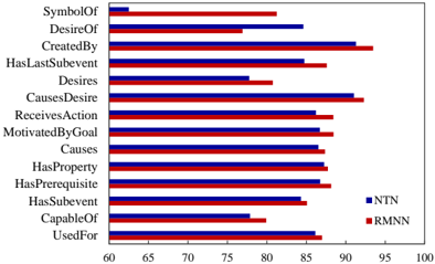| Model | Positive | Negative | total | |---------|------------|------------|---------| | NTN | 82.7 | 86.5 | 84.6 | | DNN | 84.5 | 86.9 | 85.7 | | RMNN | 85.1 | 87.1 | 86.1 | Furthermore, we show the classification accuracy of all 14 relations in CN14 for RMNN and NTN in Figure 5, which show that the accuracy of RMNN varies among different relations from 80.1% ( Desires ) to 93.5% ( CreatedBy ). We notice some commonsense relations (such as Desires , CapableOf ) are harder than the others (like CreatedBy , CausesDesire ). RMNN overtakes NTN in almost all relations. ## Knowledge Transfer Learning Knowledge transfer between various domains is a characteristic feature and crucial cornerstone of human learning. In this section, we evaluate the proposed NAM models for a Figure 5: Accuracy of different relations in CN14. <details> <summary>Image 5 Details</summary>  ### Visual Description ## Horizontal Bar Chart: Model Performance Comparison (NTN vs RMNN) ### Overview The chart compares the performance of two models, NTN (blue) and RMNN (red), across 14 relationship categories. Performance is measured on a scale from 60 to 100, with NTN consistently underperforming RMNN in most categories. ### Components/Axes - **X-axis**: Performance Score (%) (60–100) - **Y-axis**: Relationship categories (14 total) - **Legend**: - Blue = NTN - Red = RMNN - **Placement**: Legend is positioned on the right side of the chart. ### Detailed Analysis 1. **SymbolOf**: NTN (~60), RMNN (~80) 2. **DesireOf**: NTN (~85), RMNN (~75) 3. **CreatedBy**: NTN (~90), RMNN (~95) 4. **HasLastSubevent**: NTN (~85), RMNN (~88) 5. **Desires**: NTN (~75), RMNN (~80) 6. **CausesDesire**: NTN (~90), RMNN (~92) 7. **ReceivesAction**: NTN (~85), RMNN (~87) 8. **MotivatedByGoal**: NTN (~85), RMNN (~88) 9. **Causes**: NTN (~85), RMNN (~87) 10. **HasProperty**: NTN (~85), RMNN (~86) 11. **HasPrerequisite**: NTN (~85), RMNN (~88) 12. **HasSubevent**: NTN (~80), RMNN (~85) 13. **CapableOf**: NTN (~75), RMNN (~80) 14. **UsedFor**: NTN (~85), RMNN (~87) ### Key Observations - **RMNN Dominance**: RMNN outperforms NTN in 12 out of 14 categories, with margins ranging from 2% (HasProperty) to 15% (SymbolOf). - **NTN Weakness**: NTN’s lowest performance is in **SymbolOf** (~60), while RMNN’s weakest is **DesireOf** (~75). - **Consistency**: RMNN maintains higher scores across all categories, with no overlap in performance ranges except for **DesireOf** and **CapableOf**. ### Interpretation The data suggests RMNN is significantly more effective than NTN at modeling complex relationships, particularly in symbolic and causal contexts (e.g., **SymbolOf**, **CausesDesire**). NTN’s lower scores in **SymbolOf** and **Desires** may indicate limitations in handling abstract or indirect relationships. The minimal performance gap in **DesireOf** and **CapableOf** could reflect shared challenges in modeling desire-based or capability-based interactions. These results highlight RMNN’s architectural advantages in relationship extraction tasks. 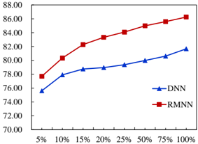</details> Figure 6: Accuracy (in %) on the test set of a new relation CausesDesire is shown as a function of used training samples from CausesDesire when updating the relation code only. (Accuracy on the original relations remains as 85.7%.) <details> <summary>Image 6 Details</summary>  ### Visual Description ## Line Graph: Performance Comparison of DNN and RMNN Models ### Overview The image depicts a line graph comparing the performance of two models, DNN (Deep Neural Network) and RMNN (Recurrent Model Neural Network), across varying input percentages (5% to 100%). The y-axis represents performance scores (70–88), while the x-axis represents input percentages. Two data series are plotted: RMNN (red squares) and DNN (blue triangles). ### Components/Axes - **X-Axis (Input Percentage)**: Labeled "5%", "10%", "15%", "20%", "25%", "50%", "75%", "100%". - **Y-Axis (Performance Score)**: Labeled from 70.00 to 88.00 in increments of 2.00. - **Legend**: Located at the bottom-right corner. - **Blue Triangles**: DNN (Deep Neural Network). - **Red Squares**: RMNN (Recurrent Model Neural Network). ### Detailed Analysis #### RMNN (Red Squares) - **Trend**: Steep upward slope, starting at ~78.00 (5%) and rising to ~86.50 (100%). - **Key Data Points**: - 5%: ~78.00 - 10%: ~80.00 - 15%: ~82.00 - 20%: ~84.00 - 25%: ~85.00 - 50%: ~85.50 - 75%: ~86.00 - 100%: ~86.50 #### DNN (Blue Triangles) - **Trend**: Gradual upward slope, starting at ~76.00 (5%) and rising to ~82.00 (100%). - **Key Data Points**: - 5%: ~76.00 - 10%: ~77.50 - 15%: ~78.50 - 20%: ~79.00 - 25%: ~79.50 - 50%: ~80.00 - 75%: ~81.00 - 100%: ~82.00 ### Key Observations 1. **Performance Gap**: RMNN consistently outperforms DNN across all input percentages, with the largest gap at lower percentages (e.g., 5%: ~2.00 difference). 2. **Slope Comparison**: RMNN’s performance increases more sharply than DNN, particularly between 5% and 25%. 3. **Convergence**: The performance gap narrows slightly at higher percentages (e.g., 100%: ~4.50 difference), but RMNN remains superior. ### Interpretation The data suggests that RMNN demonstrates significantly better performance than DNN as input percentages increase. The steeper slope of RMNN indicates it may be more sensitive to input variability or better at leveraging larger datasets. However, the narrowing gap at higher percentages implies diminishing returns for RMNN’s advantage. This could reflect architectural differences (e.g., RMNN’s recurrent design vs. DNN’s static structure) or dataset-specific optimizations. Further investigation into the input data characteristics and model training parameters would clarify these trends. </details> knowledge transfer learning scenario, where we adapt a pretrained model to an unseen relation with only a few training samples from the new relation. Here we randomly select a relation, e.g., CausesDesire in CN14 for this experiment. This relation contains only 4800 training samples and 480 test samples. During the experiments, we use all of the other 13 relations in CN14 to train baseline NAM models (both DNN and RMNN). During the transfer learning, we freeze all NAM parameters, including all weights and entity representations, and only learn a new relation code for CausesDesire from the given samples. At last, the learned relation code (along with the original NAM models) is used to classify the new samples of CausesDesire in the test set. Obviously, this transfer learning does not affect the model performance in the original 13 relations because the models are not changed. Figure 6 shows the results of knowledge transfer learning for the relation CausesDesire as we increase the training samples gradually. The result shows that RMNN performs much better than DNN in this experiment, where we can significantly improve RMNN for the new relation with only 5-20% of the total training samples for CausesDesire . This demonstrates that the structure to connect the relation code to all hidden layers leads to more effective learning of new relation codes from a relatively small number of training samples. 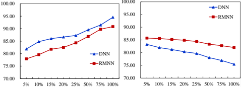Next, we also test a more aggressive learning strategy for this transfer learning setting, where we simultaneously update all the network parameters during the learning of the new relation code. The results are shown in Figure 7. This strategy can obviously improve performance more on the new relation, especially when we add more training samples. However, as expected, the performance on the original 13 relations deteriorates. The DNN improves the performance on the new relation as we use all training samples (up to 94.6%). However, the performance on the remaining 13 original relations drops dramatically from 85.6% to 75.5%. Once again, RMNN shows an advantage over DNN in this transfer learning setting, where the accuracy on the new relation increases from 77.9% to 90.8% but the accuracy on the original 13 relations only drop slightly from 85.9% to 82.0%. Figure 7: Transfer learning results by updating all network parameters. The left figure shows results on the new relation while the right figure shows results on the original relations. <details> <summary>Image 7 Details</summary>  ### Visual Description ## Line Graphs: Model Accuracy vs. Training Data Percentage ### Overview The image contains two side-by-side line graphs comparing the accuracy of two neural network models (DNN and RMNN) across varying percentages of training data. Both graphs share identical axes labels and scales but depict opposing trends: the left graph shows increasing accuracy with more training data, while the right graph shows decreasing accuracy. ### Components/Axes - **X-Axis (Horizontal):** Labeled "% of Training Data" with markers at 5%, 10%, 15%, 20%, 25%, 50%, 75%, and 100%. - **Y-Axis (Vertical):** Labeled "Accuracy (%)" with markers from 70.00 to 100.00 in 5% increments. - **Legends:** - Left graph: Blue line with triangle markers = DNN; Red line with square markers = RMNN. - Right graph: Same legend labels and markers. - **Graph Titles:** Not explicitly labeled, but contextually inferred as "Accuracy vs. Training Data" for both. ### Detailed Analysis #### Left Graph (Increasing Accuracy) - **DNN (Blue):** - Starts at ~82% accuracy at 5% training data. - Increases steadily to ~95% at 100% training data. - Key data points: - 5%: 82.00 - 10%: 85.00 - 20%: 87.00 - 50%: 91.00 - 100%: 95.00 - **RMNN (Red):** - Starts at ~78% accuracy at 5% training data. - Rises to ~91% at 100% training data. - Key data points: - 5%: 78.00 - 10%: 81.00 - 25%: 85.00 - 50%: 90.00 - 100%: 91.00 #### Right Graph (Decreasing Accuracy) - **DNN (Blue):** - Starts at ~84% accuracy at 5% training data. - Declines to ~75% at 100% training data. - Key data points: - 5%: 84.00 - 10%: 82.00 - 20%: 80.00 - 50%: 77.00 - 100%: 75.00 - **RMNN (Red):** - Starts at ~86% accuracy at 5% training data. - Declines to ~82% at 100% training data. - Key data points: - 5%: 86.00 - 10%: 85.00 - 25%: 84.00 - 50%: 83.00 - 100%: 82.00 ### Key Observations 1. **Left Graph Trends:** Both models improve accuracy as training data increases, with DNN consistently outperforming RMNN. 2. **Right Graph Trends:** Both models degrade in accuracy as training data increases, with DNN experiencing a steeper decline. 3. **Contrast:** The left and right graphs represent opposing relationships between training data percentage and accuracy, suggesting differing evaluation contexts (e.g., training vs. validation/test sets). ### Interpretation - **Left Graph:** Demonstrates typical model behavior where increased training data improves generalization, with DNN benefiting more from additional data. - **Right Graph:** Indicates potential overfitting or data leakage when training data percentage is high, as accuracy drops sharply. This could reflect evaluation on a fixed test set where more training data introduces noise or bias. - **Model Comparison:** DNN shows higher sensitivity to training data volume in both scenarios, suggesting architectural differences in handling data scarcity or abundance. - **Anomaly:** The right graph’s declining trend contradicts standard expectations, warranting investigation into data preprocessing, evaluation methodology, or model hyperparameters. </details> ## Extending NAMs for Winograd Schema Data Collection In the previous experiments sections, all the tasks already contained manually constructed training data for us. However, in many cases, if we want to realize flexible commonsense reasoning under the real world conditions, obtaining the training data can also be very challenging. More specifically, since the proposed neural association model is a typical deep learning technique, lack of training data would make it difficult for us to train a robust model. Therefore, in this paper, we make some efforts and try to mine useful data for model training. As a very first step, we are now working on collecting the cause-effect relationships between a set of common words and phrases. We believe this type of knowledge would be a key component for modeling the association relationships between discrete events. This section describes the idea for automatic cause-effect pair collection as well as the data collection results. We will first introduce the common vocabulary we created for query generation. After that, the detailed algorithm for cause-effect pair collection will be presented. Finally, the following section will present the data collection results. ## Common Vocabulary and Query Generation To avoid the data sparsity problem, we start our work by constructing a vocabulary of very common words. In our current investigations, we construct a vocabulary which contains 7500 verbs and adjectives. As shown in Table 7, this vocabulary includes 3000 verb words, 2000 verb phrases and 2500 adjective words. The procedure for constructing this vocabulary is straightforward. We first extract all words and phrases (divided by part-of-speech tags) from WordNet (Miller 1995). After conducting part-of-speech tagging on a large corpus, we then get the occurrence frequencies for all those words and phrases by scanning over the tagged corpus. Finally, we sort those words and phrases by frequency and then select the top N results. Table 7: Common vocabulary constructed for mining causeeffect event pairs. 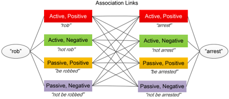| Set | Category | Size | |-------|-----------------|--------| | 1 | Verb words | 3000 | | 2 | Verb phrases | 2000 | | 3 | Adjective words | 2500 | Query Generation Based on the common vocabulary, we generate search queries by pairing any two words (or phrases). Currently we only focus on extracting the association relationships between verbs and adjectives. Even for this small vocabulary, the search space is very large (7.5K by 7.5K leads to tens of millions pairs). In this work, we define several patterns for each word or phrase based on two popular semantic dimensions: 1) positive-negative, 2) activepassive (Osgood 1952). Using the verbs rob and arrest for example, each of them contains 4 patterns, i.e. (active, positive), (active, negative), (passive, positive) and (passive, negative). Therefore, the query formed by rob and arrest would contain 16 possible dimensions, as shown in Figure 8. The task of mining the cause-effect relationships for any two words or phrases then becomes the task of getting the number of occurrences for all the possible links. Text corpus Vocab Sentences Results Figure 8: Typical 16 dimensions for a typical query. <details> <summary>Image 8 Details</summary>  ### Visual Description ## Diagram: Association Links Between "rob" and "arrest" ### Overview The diagram illustrates bidirectional association links between two core concepts: "rob" and "arrest." Each concept is represented by an oval node, connected to four colored rectangular nodes that encode grammatical (active/passive) and semantic (positive/negative) variations. Black lines represent association links between all nodes, forming a fully connected bipartite graph. ### Components/Axes - **Legend**: Located at the top center, labeled "Association Links." - **Nodes**: - **Left Oval**: Labeled "rob" (black text, white background). - **Right Oval**: Labeled "arrest" (black text, white background). - **Colored Rectangles**: - **Red**: "Active, Positive" (white text). - **Green**: "Active, Negative" (black text). - **Yellow**: "Passive, Positive" (black text). - **Purple**: "Passive, Negative" (black text). - **Labels**: Each rectangle contains a verb form (e.g., "rob," "not rob," "be robbed," "not be robbed") and its grammatical/semantic classification. - **Connections**: Black lines link all nodes bidirectionally, creating a dense network. ### Detailed Analysis - **Left Oval ("rob")**: - **Active, Positive**: "rob" - **Active, Negative**: "not rob" - **Passive, Positive**: "be robbed" - **Passive, Negative**: "not be robbed" - **Right Oval ("arrest")**: - **Active, Positive**: "arrest" - **Active, Negative**: "not arrest" - **Passive, Positive**: "be arrested" - **Passive, Negative**: "not be arrested" - **Association Links**: - Every node is connected to every node in the opposite oval (e.g., "rob" connects to "arrest," "not arrest," "be arrested," etc.). - No self-connections within the same oval. ### Key Observations 1. **Bidirectional Completeness**: All possible combinations of "rob" and "arrest" variations are linked, suggesting a holistic semantic relationship. 2. **Color Coding**: Red (positive) and green (negative) dominate active forms, while yellow (positive) and purple (negative) dominate passive forms. 3. **Semantic Symmetry**: Passive forms ("be robbed," "be arrested") mirror active forms but with inverted agency. ### Interpretation This diagram models the polysemous relationship between "rob" and "arrest," emphasizing how grammatical transformations (active/passive) and semantic oppositions (positive/negative) create a network of associations. The bidirectional links imply that each variation of "rob" semantically interacts with all variations of "arrest," and vice versa. For example: - "rob" (active positive) is linked to "arrest" (active positive), suggesting a shared core concept of intentional action. - "not rob" (active negative) connects to "not be arrested" (passive negative), highlighting inverse relationships. - Passive forms ("be robbed," "be arrested") retain positive polarity despite inverted agency, indicating focus on the action’s occurrence rather than the agent. The structure reflects linguistic complexity, where verbs encode both action direction (active/passive) and semantic valence (positive/negative), with associations spanning all combinations. This could inform NLP tasks like semantic role labeling or verb sense disambiguation. </details> ## Automatic Cause-Effect Pair Collection Based on the created queries, in this section, we present the procedures for extracting cause-effect pairs from large unstructured texts. The overall system framework is shown in Figure 9. 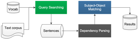Query Searching The goal of query searching is to find all the possible sentences that may contain the input queries. Since the number of queries is very large, we structure all the queries as a hashmap and conduct string matching during text scanning. In detail, the searching program starts by Figure 9: Automatic pair collection system framework. <details> <summary>Image 9 Details</summary>  ### Visual Description ## Flowchart: Text Processing Pipeline ### Overview The image depicts a multi-stage text processing pipeline with interconnected components. The flowchart uses color-coded blocks (green, blue, gray) to represent distinct processing stages, with arrows indicating data flow direction. Vocabulary and text corpus inputs feed into the system, culminating in structured results. ### Components/Axes 1. **Input Sources**: - **Vocab**: Circular container (left side) - **Text corpus**: Rectangular document icon (bottom-left) 2. **Processing Stages**: - **Query Searching**: Green rectangle (central-left) - **Sentences**: Cylinder container (below Query Searching) - **Dependency Parsing**: Dark gray rectangle (center-right) - **Subject-Object Matching**: Blue rectangle (top-right) 3. **Output**: - **Results**: Cylinder container (far right) 4. **Color Legend**: - Green: Query Searching - Blue: Subject-Object Matching - Gray: Dependency Parsing ### Detailed Analysis 1. **Flow Direction**: - **Left to Right**: Primary data flow from inputs to outputs - **Bottom to Top**: Secondary vertical flow from Sentences to Dependency Parsing 2. **Component Relationships**: - **Vocab/Text corpus** → **Query Searching** (green) - **Query Searching** → **Sentences** (cylinder) - **Sentences** → **Dependency Parsing** (gray) - **Dependency Parsing** → **Subject-Object Matching** (blue) - **Subject-Object Matching** → **Results** 3. **Spatial Grounding**: - Inputs clustered on the left - Processing stages form a diagonal progression from bottom-left (green) to top-right (blue) - Results container isolated on the far right ### Key Observations 1. **Modular Design**: Each processing stage operates as an independent module with clear input/output boundaries 2. **Color Coding**: Distinct colors prevent ambiguity between processing stages 3. **Bidirectional Flow**: While primary flow is left→right, the vertical connection between Sentences and Dependency Parsing creates a feedback loop 4. **Result Isolation**: Final output is physically separated from processing stages, emphasizing output purity ### Interpretation This flowchart represents a natural language processing (NLP) pipeline where: 1. **Vocabulary and text corpus** serve as foundational inputs 2. **Query Searching** (green) acts as the initial filtering/extraction stage 3. **Dependency Parsing** (gray) introduces structural analysis of sentences 4. **Subject-Object Matching** (blue) represents the core relationship extraction component 5. The vertical connection between Sentences and Dependency Parsing suggests iterative refinement of linguistic analysis 6. The isolated Results container implies a final validation or formatting stage before output The color-coded modular design emphasizes separation of concerns, while the bidirectional flow acknowledges the iterative nature of NLP processing. The system architecture prioritizes clear data provenance, with each stage building upon the previous while maintaining distinct functional responsibilities. </details> conducting lemmatizing, part-of-speech tagging and dependency parsing on the source corpus. After it, we scan the corpus from the begining to end. When dealing with each sentence, we will try to find the matched words (or phrases) using the hashmap. This strategy help us to reduce the search complexity to be linear with the size of corpus, which has been proved to be very efficient in our experiments. 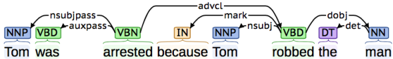Association Links 'rob' Active, Positive Active, Negative Passive, Positive Passive, Negative 'arrest' Active, Positive Active, Negative Passive, Positive Passive, Negative Subject-Object Matching Based on the dependency parsing results, once we find one phrase of a query, we would check whether that phrase is associated with at least one subject or object in the corresponding sentence or not. At the same time, we record whether the phrase was positive or negative, active or passive. Moreover, for helping us to decide the cause-effect relationships, we would check whether the phrase is linked with some connective words or not. Typical connective words used in this work are because and if . To finally extract the cause-effect pairs, we design a simple subject-object matching rule, which is similar to the work of (Peng, Khashabi, and Roth 2015). 1) If the two phrases in one query share the same subject , the relationship between them is then straightforward; 2) If the subject of one phrase is the object of the other phrase, then we need to apply the passive pattern to the phrase related to the object . This subject-object matching idea is similar to the work proposed in (Peng, Khashabi, and Roth 2015). Using query ( arrest , rob ) as an example. Once we find sentence 'Tom was arrested because Tom robbed the man' , we obtain its dependency parsing result as shown in Figure 10. The verb arrest and rob share a same subject, and the pattern for arrest is passive, we will add the occurrence of the corresponding association link, i.e. link from the (active,positive) pattern of rob to the (passive,positive) pattern of arrest , by 1. Figure 10: Dependency parsing result of sentence 'Tom was arrested because Tom robbed the man' . <details> <summary>Image 10 Details</summary>  ### Visual Description Icon/Small Image (393x59) </details> ## Data Collection Results Table 8 shows the corpora we used for collecting the causeeffect pairs and the corresponding data collection results. We extract approximately 240,000 pairs from different corpora. Table 8: Data collection results on different corpora. | Corpus | # Result pairs | |------------------------------|------------------| | Gigaword (Graff et al. 2003) | 117,938 | | Novels (Zhu et al. 2015) | 129,824 | | CBTest (Hill et al. 2015) | 4,167 | | BNC (Burnard 1995) | 2,128 | ## Winograd Schema Challenge Based on all the experiments described in the previous sections, we could conclude that the neural association model has the potential to be effective in commonsense reasoning. To further evaluate the effectiveness of the proposed neural association model, in this paper, we conduct experiments on solving the complex Winograd Schema challenge problems (Levesque, Davis, and Morgenstern 2011; Morgenstern, Davis, and Ortiz Jr 2016). Winograd Schema is a commonsense reasoning task proposed in recent years, which has been treated as an alternative to the Turing Test (Turing 1950). This is a new AI task and it would be very interesting to see whether neural network methods are suitable for solving this problem. This section then describes the progress we have made in attempting to meet the Winograd Schema Challenge. For making clear what is the main task of the Winograd Schema , we will firstly introduce it at a high level. Afterwards, we will introduce the system framework as well as all the corresponding modules we proposed to automatically solve the Winograd Schema problems. Finally, experiments and discussions on a human annotated causeeffect dataset and discussion will be presented. ## Winograd Schema The Winograd Schema (WS) evaluates a system's commonsense reasoning ability based on a traditional, very difficult natural language processing task: coreference resolution (Levesque, Davis, and Morgenstern 2011; Saba 2015). The Winograd Schema problems are carefully designed to be a task that cannot be easily solved without commonsense knowledge. In fact, even the solution of traditional coreference resolution problems relies on semantics or world knowledge (Rahman and Ng 2011; Strube 2016). For describing the WS in detail, here we just copy some words from (Levesque, Davis, and Morgenstern 2011). A WS is a small reading comprehension test involving a single binary question. Here are two examples: - The trophy would not fit in the brown suitcase because it was too big. What was too big? - -Answer 0: the trophy - -Answer 1: the suitcase - Joan made sure to thank Susan for all the help she had given. Who had given the help? - -Answer 0: Joan - -Answer 1: Susan The correct answers here are obvious for human beings. In each of the questions, the corresponding WS has the following four features: 1. Two parties are mentioned in a sentence by noun phrases. They can be two males, two females, two inanimate objects or two groups of people or objects. 2. A pronoun or possessive adjective is used in the sentence in reference to one of the parties, but is also of the right sort for the second party. In the case of males, it is 'he/him/his'; for females, it is 'she/her/her' for inanimate object it is 'it/it/its,' and for groups it is 'they/them/their.' 3. The question involves determining the referent of the pronoun or possessive adjective. Answer 0 is always the first party mentioned in the sentence (but repeated from the sentence for clarity), and Answer 1 is the second party. 4. There is a word (called the special word) that appears in the sentence and possibly the question. When it is replaced by another word (called the alternate word), everything still makes perfect sense, but the answer changes. Solving WS problems is not easy since the required commonsense knowledge is quite difficult to collect. In the following sections, we are going to describe our work on solving the Winograd Schema problems via neural network methods. ## System Framework In this paper, we propose that the commonsense knowledge required in many Winograd Schema problems could be formulized as some association relationships between discrete events. Using sentence ' Joan made sure to thank Susan for all the help she had given ' as an example, the commonsense knowledge is that the man who receives help should thank to the man who gives help to him. We believe that by modeling the association between event receive help and thank , give help and thank , we can make the decision by comparing the association probability Pr( thank | receive help ) and Pr( thank | give help ) . If the models are well trained, we should get the inequality Pr( thank | receive help ) > Pr( thank | give help ) . Following this idea, we propose to utilize the data constructed from the previous section and extend the NAM models for solving WS problems. Here we design two frameworks for training NAM models. 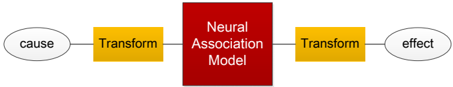relation - TransMat -NAM: We design to apply four linear transformation matrices, i.e., matrices of (active, positive), (active, negative), (passive, positive) and (passive, negative), for transforming both the cause event and the effect event. After it, we then use NAM for model the causeeffect association relationship between any cause and effect events. 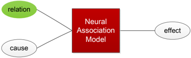cause effect Neural Association Model - RelationVec -NAM: On the other hand, in this configuration, we treat all the typical 16 dimensions shown in Figure 8 as distinct relations. So there are 16 relation vectors Figure 11: The model framework for TransMat -NAM. <details> <summary>Image 11 Details</summary>  ### Visual Description ## Flowchart: Causal Process Mediated by Neural Association Model ### Overview The image depicts a sequential causal process diagram with four key components: a "cause" (left), two "Transform" steps (yellow rectangles), a central "Neural Association Model" (red rectangle), and an "effect" (right). Arrows indicate directional flow between elements. ### Components/Axes - **Left Oval**: Labeled "cause" (gray background). - **First Yellow Rectangle**: Labeled "Transform" (black text). - **Central Red Rectangle**: Labeled "Neural Association Model" (white text). - **Second Yellow Rectangle**: Labeled "Transform" (black text). - **Right Oval**: Labeled "effect" (gray background). - **Arrows**: Connect components in sequence (left to right). ### Detailed Analysis - **Cause → First Transform**: Arrow originates from "cause" oval, pointing to the first "Transform" rectangle. - **First Transform → Neural Association Model**: Arrow connects the first "Transform" to the central "Neural Association Model." - **Neural Association Model → Second Transform**: Arrow links the model to the second "Transform" rectangle. - **Second Transform → Effect**: Final arrow directs from the second "Transform" to the "effect" oval. ### Key Observations 1. The process is linear and unidirectional, with no feedback loops. 2. The "Neural Association Model" acts as the central processing node. 3. Both "Transform" steps are identical in labeling and color, suggesting equivalence in function. ### Interpretation This diagram illustrates a causal chain where an initial "cause" undergoes two transformation steps before being processed by a neural association model, ultimately producing an "effect." The use of identical "Transform" labels implies that both steps serve similar roles, potentially as preprocessing or feature extraction stages. The red "Neural Association Model" is visually emphasized, indicating its critical role in mediating the relationship between transformations and the final outcome. The absence of numerical data or probabilistic elements suggests this is a conceptual or architectural representation rather than a statistical model. **Note**: No numerical values, axes, or legends are present. The diagram focuses on structural relationships and process flow. </details> in the corresponding NAM models. Currently we use the RMNN structure for NAM. Figure 12: The model framework for RelationVec -NAM. <details> <summary>Image 12 Details</summary>  ### Visual Description ## Diagram: Neural Association Model Architecture ### Overview The diagram illustrates a conceptual model of neural association, depicting relationships between "cause," "relation," and "effect" through a central processing unit labeled "Neural Association Model." ### Components/Axes - **Central Node**: A red square labeled "Neural Association Model" (positioned centrally). - **Input Nodes**: - Green oval labeled "relation" (top-left of the central node). - White oval labeled "cause" (bottom-left of the central node). - **Output Node**: - White oval labeled "effect" (right of the central node). - **Connections**: - Black lines connect "relation" and "cause" to the central node. - A single black line connects the central node to "effect." ### Detailed Analysis - **Textual Labels**: - "Neural Association Model" (central red square). - "relation" (green oval, top-left). - "cause" (white oval, bottom-left). - "effect" (white oval, right). - **Color Coding**: - "relation" is uniquely green, while "cause" and "effect" are white. - No explicit legend is present, but color differentiation suggests "relation" may represent a distinct input type. ### Key Observations 1. The model processes two inputs ("cause" and "relation") to produce a single output ("effect"). 2. The green color of "relation" may imply a qualitative or contextual input, contrasting with the neutral white of "cause." 3. The unidirectional flow from inputs to output suggests a deterministic relationship. ### Interpretation The diagram represents a simplified causal inference framework where the "Neural Association Model" integrates contextual ("relation") and direct ("cause") inputs to generate an "effect." The use of color (green for "relation") hints at potential prioritization or weighting of contextual factors in the model's processing. This structure aligns with cognitive science models of associative learning, where neural networks link stimuli (cause/relation) to outcomes (effect). No numerical data or trends are present; the diagram focuses on conceptual relationships rather than quantitative analysis. </details> cause effect Neural Association Model Transform Transform Training the NAM models based on these two configurations is straightforward. All the network parameters, including the relation vectors and the linear transformation matrices, are learned by the standard stochastic gradient descend algorithm. ## Experiments In this section, we will introduce our current experiments on solving the Winograd Schema problems. We will first select a cause-effect dataset constructed from the standard WS dataset. Subsequently, experimental setup will be described in detail. After presenting the experimental results, discussions would be made at the end of this section. Cause-Effect Dataset Labelling In this paper, based on the WS dataset available at http: //www.cs.nyu.edu/faculty/davise/papers/ WinogradSchemas/WS.html , we labelled 78 causeeffect problems among all 278 available WS questions for our experiments. Table 9 shows some typical examples. For each WS problem, we label three verb (or adjective) phrases for the corresponding two parities and the pronoun. In the labelled phrases, we also record the corresponding patterns for each word respectively. Using word lift for example, we will generate lift for its active and positive pattern, not lift for its active and negative pattern, be lifted for its passive and positive pattern, and not be lifted for its passive and negative pattern. For example, in sentence ' The man couldn't lift his son because he was so weak ', we identify weak , not lift and not be lifted for he , the man and son resspectively. The commonsense is that somebody who is weak would more likely to has the effect not lift rather than not be lifted . The main work of NAM for solving this problem is to calculate the association probability between these phrases. Experimental setup The setup for NAM on this causeeffect task is similar to the settings on the previous tasks. For representing the phrases in neural association models, we use the bag-of-word (BOW) approach for composing phrases from pre-trained word vectors. Since the vocabulary we use in this experiment contains only 7500 common verbs and adjectives, there are some out-of-vocabulary (OOV) words in some phrases. Based on the BOW method, a phrase would be useless if all the words it contains are OOV. In this paper, we remove all the testing samples with useless phrases which results in 70 testing cause-effect samples. For network settings, we set the embedding size to 50 and the Table 9: Examples of the Cause-Effect dataset labelled from the Winograd Schema Challenge. | Schema texts | Verb/Adjective 1 | Verb/Adjective 2 | Verb/Adjective 3 | |---------------------------------------------------------------------------------|--------------------|--------------------|--------------------| | The man couldn't lift his son because he was so weak | weak | not lift | not be lifted | | The man couldn't lift his son because he was so heavy | heavy | not lift | not be lifted | | The fish ate the worm. it was tasty | tasty | eat | be eaten | | The fish ate the worm. it was hungry | hungry | eat | be eaten | | Mary tucked her daughter Anne into bed, so that she could sleep | tuck into bed | be tucked into bed | sleep | | Mary tucked her daughter Anne into bed, so that she could work | tuck into bed | be tucked into bed | work | | Tom threw his schoolbag down to ray after he reached the top of the stairs | reach top | throw down | be thrown down | | Tom threw his schoolbag down to ray after he reached the bottom of the stairs | reach bottom | throw down | be thrown down | | Jackson was greatly influenced by Arnold, though he lived two centuries earlier | live earlier | influence | be influenced | | Jackson was greatly influenced by Arnold, though he lived two centuries later | live later | influence | be influenced | dimension of relation vectors to 50. We set 2 hidden layers for the NAM models and all the hidden layer sizes are set to 100. The learning rate is set to 0.01 for all the experiments. At the same time, to better control the model training, we set the learning rates for learning all the embedding matrices and the relation vectors to 0.025. Negative sampling is very important for model training for this task. In the TransMat -NAM system, we generate negative samples by randomly selecting different patterns with respect to the pattern of the effect event in the positive samples. For example, if the positive training sample is ' hungry (active, positive) causes eat (active, positive) ', we may generate negative samples like ' hungry (active, positive) causes eat (passive, positive) ', or ' hungry (active, positive) causes eat (active, negative) '. In the RelationVec -NAM system, the negative sampling method is much more straightforward, i.e., we will randomly select a different effect event from the whole vocabulary. In the example shown here, the possible negative sample would be ' hungry (active, positive) causes happy (active, positive) ', or ' hungry (active, positive) causes talk (active, positive) ' and so on. Results The experimental results are shown in Table 10. From the results, we find that the proposed NAM models achieve about 60% accuracy on the cause-effect dataset constructed from Winograd Schemas . More specifically, the RelationVec -NAM system performs slightly better than the TransMat -NAM system. Table 10: Results of NAMs on the Winograd Schema CauseEffect dataset. | Model | Accuracy (%) | |------------------|----------------| | TransMat -NAM | 58.6 (41 / 70) | | RelationVec -NAM | 61.4 (43 / 70) | In the testing results, we find the NAM performs well on some testing examples. For instance, in the call phone scenario, the proposed NAM generates the corresponding association probabilities as follows. - Paul tried to call George on the phone, but he wasn't successful. Who was not successful? - Paul tried to call George on the phone, but he wasn't available. Who was not available? - Paul: Pr( not successful | call ) = 0.7299 - George: Pr( not successful | be called ) = 0.5430 - Answer: Paul - Paul: Pr( not available | call ) = 0.6859 - George: Pr( not available | be called ) = 0.8306 - Answer: George For these testing examples, we find our model can answer the questions by correctly calculating the association probabilities. The probability Pr( not successful | call ) is larger than Pr( not successful | be called ) while the probability Pr( not available | call ) is smaller than Pr( not available | be called ) . Those simple inequality relationships between the association probabilities are very reasonable in our commonsense. Here are some more examples: - Jim yelled at Kevin because he was so upset. Who was upset? - -Jim: Pr( yell | be upset ) = 0.9296 - -Kevin: Pr( be yelled | be upset ) = 0.8785 - -Answer: Jim - Jim comforted Kevin because he was so upset. Who was upset? - -Answer: Kevin - Jim: Pr( comfort | be upset ) = 0.0282 - Kevin: Pr( be comforted | be upset ) = 0.5657 This example also conveys some commonsense knowledge in our daily life. We all know that somebody who is upset would be more likely to yell at other people. Meanwhile, it is also more likely that they would be be comforted by other people. ## Conclusions In this paper, we have proposed neural association models (NAM) for probabilistic reasoning. We use neural networks to model association probabilities between any two events in a domain. In this work, we have investigated two model structures, namely DNN and RMNN, for NAMs. Experimental results on several reasoning tasks have shown that both DNNs and RMNNs can outperform the existing methods. This paper also reports some preliminary results to use NAMs for knowledge transfer learning. We have found that the proposed RMNN model can be quickly adapted to a new relation without sacrificing the performance in the original relations. After proving the effectiveness of the NAM models, we apply it to solve more complex commonsense reasoning problems, i.e., the Winograd Schemas (Levesque, Davis, and Morgenstern 2011). To support model training in this task, we propose a straightforward method to collect associative phrase pairs from text corpora. Experiments conducted on a set of Winograd Schema problems have indicated the neural association model does solve some problems successfully. However, it is still a long way to finally achieving automatic commonsense reasoning. ## Acknowledgments We want to thank Prof. Gary Marcus of New York University for his useful comments on commonsense reasoning. Wealso want to thank Prof. Ernest Davis, Dr. Leora Morgenstern and Dr. Charles Ortiz for their wonderful organizations for making the first Winograd Schema Challenge happen. This paper was supported in part by the Science and Technology Development of Anhui Province, China (Grants No. 2014z02006), the Fundamental Research Funds for the Central Universities (Grant No. WK2350000001) and the Strategic Priority Research Program of the Chinese Academy of Sciences (Grant No. XDB02070006). ## References - [Bengio et al. 2003] Bengio, Y.; Ducharme, R.; Vincent, P.; and Janvin, C. 2003. A neural probabilistic language model. The Journal of Machine Learning Research 3:1137-1155. - [Bordes et al. 2012] Bordes, A.; Glorot, X.; Weston, J.; and Bengio, Y. 2012. Joint learning of words and meaning representations for open-text semantic parsing. In Proceedings of AISTATS , 127-135. - [Bordes et al. 2013] Bordes, A.; Usunier, N.; Garcia-Duran, A.; Weston, J.; and Yakhnenko, O. 2013. Translating embeddings for modeling multi-relational data. In Proceedings of NIPS , 2787-2795. - [Bowman et al. 2015] Bowman, S. R.; Angeli, G.; Potts, C.; and Manning, C. D. 2015. A large annotated corpus for learning natural language inference. arXiv preprint arXiv:1508.05326 . - [Bowman 2013] Bowman, S. R. 2013. Can recursive neural tensor networks learn logical reasoning? arXiv preprint arXiv:1312.6192 . - [Burnard 1995] Burnard, L. 1995. Users reference guide british national corpus version 1.0. - [Collobert et al. 2011] Collobert, R.; Weston, J.; Bottou, L.; Karlen, M.; Kavukcuoglu, K.; and Kuksa, P. 2011. Natural language processing (almost) from scratch. The Journal of Machine Learning Research 12:2493-2537. - [Getoor 2007] Getoor, L. 2007. Introduction to statistical relational learning . MIT press. - [Glorot and Bengio 2010] Glorot, X., and Bengio, Y. 2010. Understanding the difficulty of training deep feedforward neural networks. In Proceedings of AISTATS , 249-256. - [Graff et al. 2003] Graff, D.; Kong, J.; Chen, K.; and Maeda, K. 2003. English gigaword. Linguistic Data Consortium, Philadelphia . - [Hill et al. 2015] Hill, F.; Bordes, A.; Chopra, S.; and Weston, J. 2015. The goldilocks principle: Reading children's books with explicit memory representations. arXiv preprint arXiv:1511.02301 . - [Hinton et al. 2012] Hinton, G. E.; Srivastava, N.; Krizhevsky, A.; Sutskever, I.; and Salakhutdinov, R. R. 2012. Improving neural networks by preventing co-adaptation of feature detectors. arXiv preprint arXiv:1207.0580 . - [Hornik, Stinchcombe, and White 1990] Hornik, K.; Stinchcombe, M.; and White, H. 1990. Universal approximation of an unknown mapping and its derivatives using multilayer feedforward networks. Neural networks 3(5):551-560. - [Jensen 1996] Jensen, F. V. 1996. An introduction to Bayesian networks , volume 210. UCL press London. - [Koller and Friedman 2009] Koller, D., and Friedman, N. 2009. Probabilistic graphical models: principles and techniques . MIT press. - [LeCun, Bengio, and Hinton 2015] LeCun, Y.; Bengio, Y.; and Hinton, G. 2015. Deep learning. Nature 521(7553):436-444. - [Levesque, Davis, and Morgenstern 2011] Levesque, H. J.; Davis, E.; and Morgenstern, L. 2011. The winograd schema challenge. In AAAI Spring Symposium: Logical Formalizations of Commonsense Reasoning . - [Lin et al. 2015] Lin, Y.; Liu, Z.; Sun, M.; Liu, Y.; and Zhu, X. 2015. Learning entity and relation embeddings for knowledge graph completion. In Proceedings of AAAI . - [Liu and Singh 2004] Liu, H., and Singh, P. 2004. Conceptnet: a practical commonsense reasoning toolkit. BT technology journal 22(4):211-226. - [McCarthy 1986] McCarthy, J. 1986. Applications of circumscription to formalizing common-sense knowledge. Artificial Intelligence 28(1):89-116. - [Mikolov et al. 2013] Mikolov, T.; Chen, K.; Corrado, G.; and Dean, J. 2013. Efficient estimation of word representations in vector space. arXiv preprint arXiv:1301.3781 . - [Miller 1995] Miller, G. A. 1995. Wordnet: a lexical database for english. Communications of the ACM 38(11):39-41. - [Minsky 1988] Minsky, M. 1988. Society of mind . Simon and Schuster. - [Morgenstern, Davis, and Ortiz Jr 2016] Morgenstern, L.; Davis, E.; and Ortiz Jr, C. L. 2016. Planning, executing, and evaluating the winograd schema challenge. AI Magazine 37(1):50-54. - [Mueller 2014] Mueller, E. T. 2014. Commonsense Reasoning: An Event Calculus Based Approach . Morgan Kaufmann. - [Nair and Hinton 2010] Nair, V., and Hinton, G. E. 2010. Rectified linear units improve restricted boltzmann machines. In Proceedings of ICML , 807-814. - [Neapolitan 2012] Neapolitan, R. E. 2012. Probabilistic reasoning in expert systems: theory and algorithms . CreateSpace Independent Publishing Platform. - [Nickel et al. 2015] Nickel, M.; Murphy, K.; Tresp, V.; and Gabrilovich, E. 2015. A review of relational machine learning for knowledge graphs. arXiv preprint arXiv:1503.00759 . - [Nickel, Tresp, and Kriegel 2012] Nickel, M.; Tresp, V.; and Kriegel, H.-P. 2012. Factorizing YAGO: scalable machine learning for linked data. In Proceedings of WWW , 271-280. ACM. - [Osgood 1952] Osgood, C. E. 1952. The nature and measurement of meaning. Psychological bulletin 49(3):197. - [Pearl 1988] Pearl, J. 1988. Probabilistic reasoning in intelligent systems: Networks of plausible reasoning. - [Peng, Khashabi, and Roth 2015] Peng, H.; Khashabi, D.; and Roth, D. 2015. Solving hard coreference problems. Urbana 51:61801. - [Rahman and Ng 2011] Rahman, A., and Ng, V. 2011. Coreference resolution with world knowledge. In Proceedings of the 49th Annual Meeting of the Association for Computational Linguistics: Human Language TechnologiesVolume 1 , 814-824. Association for Computational Linguistics. - [Richardson and Domingos 2006] Richardson, M., and Domingos, P. 2006. Markov logic networks. Machine learning 62(1-2):107-136. - [Saba 2015] Saba, W. 2015. On the winograd schema challenge. - [Socher et al. 2013] Socher, R.; Chen, D.; Manning, C. D.; and Ng, A. 2013. Reasoning with neural tensor networks for knowledge base completion. In Proceedings of NIPS , 926-934. - [Strube 2016] Strube, M. 2016. The (non) utility of semantics for coreference resolution (corbon remix). In NAACL 2016 workshop on Coreference Resolution Beyond OntoNotes . - [Turing 1950] Turing, A. M. 1950. Computing machinery and intelligence. Mind 59(236):433-460. - [Wang et al. 2014] Wang, Z.; Zhang, J.; Feng, J.; and Chen, Z. 2014. Knowledge graph embedding by translating on hyperplanes. In Proceedings of AAAI , 1112-1119. Citeseer. - [Xue et al. 2014] Xue, S.; Abdel-Hamid, O.; Jiang, H.; Dai, L.; and Liu, Q. 2014. Fast adaptation of deep neural network based on discriminant codes for speech recognition. Audio, Speech, and Language Processing, IEEE/ACM Trans. on 22(12):1713-1725. - [Zhu et al. 2015] Zhu, Y.; Kiros, R.; Zemel, R.; Salakhutdinov, R.; Urtasun, R.; Torralba, A.; and Fidler, S. 2015. Aligning books and movies: Towards story-like visual explanations by watching movies and reading books. In Proceedings of the IEEE International Conference on Computer Vision , 19-27.