1609.00672v5

## The Inflation Technique for Causal Inference with Latent Variables Elie Wolfe, 1, ∗ Robert W. Spekkens, 1, † and Tobias Fritz 1, ‡ 1 Perimeter Institute for Theoretical Physics, Waterloo, Ontario, Canada, N2L 2Y5 (Dated: July 24, 2019) The problem of causal inference is to determine if a given probability distribution on observed variables is compatible with some causal structure. The difficult case is when the causal structure includes latent variables. We here introduce the inflation technique for tackling this problem. An inflation of a causal structure is a new causal structure that can contain multiple copies of each of the original variables, but where the ancestry of each copy mirrors that of the original. To every distribution of the observed variables that is compatible with the original causal structure, we assign a family of marginal distributions on certain subsets of the copies that are compatible with the inflated causal structure. It follows that compatibility constraints for the inflation can be translated into compatibility constraints for the original causal structure. Even if the constraints at the level of inflation are weak, such as observable statistical independences implied by disjoint causal ancestry, the translated constraints can be strong. We apply this method to derive new inequalities whose violation by a distribution witnesses that distribution's incompatibility with the causal structure (of which Bell inequalities and Pearl's instrumental inequality are prominent examples). We describe an algorithm for deriving all such inequalities for the original causal structure that follow from ancestral independences in the inflation. For three observed binary variables with pairwise common causes, it yields inequalities that are stronger in at least some aspects than those obtainable by existing methods. We also describe an algorithm that derives a weaker set of inequalities but is more efficient. Finally, we discuss which inflations are such that the inequalities one obtains from them remain valid even for quantum (and post-quantum) generalizations of the notion of a causal model. ∗ ewolfe@perimeterinstitute.ca † rspekkens@perimeterinstitute.ca ‡ tfritz@perimeterinstitute.ca ## CONTENTS | I. Introduction | 2 | |--------------------------------------------------------------------------------------------------------|-----| | II. Basic Definitions of Causal Models and Compatibility | 5 | | III. The Inflation Technique for Causal Inference | 6 | | A. Inflations of a Causal Model | 6 | | B. Witnessing Incompatibility | 8 | | C. Deriving Causal Compatibility Inequalities | 12 | | IV. Systematically Witnessing Incompatibility and Deriving Inequalities | 15 | | A. Identifying the AI-Expressible Sets | 17 | | B. The Marginal Problem and its Solution | 19 | | C. A List of Causal Compatibility Inequalities for the Triangle scenario | 20 | | D. Causal Compatibility Inequalities via Hardy-type Inferences from Logical Tautologies | 21 | | V. Further Prospects for the Inflation Technique | 24 | | A. Appealing to d -Separation Relations in the Inflated Causal Structure beyond Ancestral Independance | 24 | | B. Imposing Symmetries from Copy-Index-Equivalent Subgraphs of the Inflated Causal Structure | 25 | | C. Incorporating Nonlinear Constraints | 25 | | D. Implications of the Inflation Technique for Quantum Physics and Generalized Probabilistic Theories | 26 | | VI. Conclusions | 29 | | Acknowledgments | 30 | | A. Algorithms for Solving the Marginal Constraint Problem | 31 | | B. Explicit Marginal Description Matrix of the Cut Inflation with Binary Observed Variables | 32 | | C. Constraints on Marginal Distributions from Copy-Index Equivalence Relations | 33 | | D. Using the Inflation Technique to Certify a Causal Structure as 'Interesting' | 35 | | 1. Certifying that Henson-Lal-Pusey's Causal Structure #16 is 'Interesting' | 35 | | 2. Deriving a Causal Compatibility Inequality for HLP's Causal Structure #16 | 37 | | 3. Certifying that Henson-Lal-Pusey's Causal Structures #15 and #20 are 'Interesting' | 38 | | E. The Copy Lemma and Non-Shannon type Entropic Inequalities | 39 | | F. Causal Compatibility Inequalities for the Triangle Scenario in Machine-Readable Format | 40 | | G. Recovering the Bell Inequalities from the Inflation Technique | 41 | ## I. INTRODUCTION Given a joint probability distribution of some observed variables, the problem of causal inference is to determine which hypotheses about the causal mechanism can explain the given distribution. Here, a causal mechanism may comprise both causal relations among the observed variables, as well as causal relations among these and a number of unobserved variables, and among unobserved variables only. Causal inference has applications in all areas of science that use statistical data and for which causal relations are important. Examples include determining the effectiveness of medical treatments, sussing out biological pathways, making data-based social policy decisions, and possibly even in developing strong machine learning algorithms [1-5]. A closely related type of problem is to determine, for a given set of causal relations, the set of all distributions on observed variables that can be generated from them. A special case of both problems is the following decision problem: given a probability distribution and a hypothesis about the causal relations, determine whether the two are compatible: could the given distribution have been generated by the hypothesized causal relations? This is the problem that we focus on. We develop necessary conditions for a given distribution to be compatible with a given hypothesis about the causal relations. In the simplest setting, the causal hypothesis consists of a directed acyclic graph (DAG) all of whose nodes correspond to observed variables. In this case, obtaining a verdict on the compatibility of a given distribution with the causal hypothesis is simple: the compatibility holds if and only if the distribution is Markov with respect to the DAG, which is to say that the distribution features all of the conditional independence relations that are implied by d -separation relations among variables in the DAG. The DAGs that are compatible with the given distribution can be determined algorithmically [1]. 1 A significantly more difficult case is when one considers a causal hypothesis which consists of a DAG some of whose nodes correspond to latent (i.e., unobserved) variables, so that the set of observed variables corresponds to a strict subset of the nodes of the DAG. This case occurs, e.g., in situations where one needs to deal with the possible presence of unobserved confounders, and thus is particularly relevant for experimental design in applications. With latent variables, the condition that all of the conditional independence relations among the observed variables that are implied by d -separation relations in the DAG is still a necessary condition for compatibility of a given such distribution with the DAG, but in general it is no longer sufficient, and this is what makes the problem difficult. Whenever the observed variables in a DAG have finite cardinality 2 , one may also restrict the latent variables in the causal hypothesis to be of finite cardinality as well, without loss of generality [6]. As such, the mathematical problem which one must solve to infer the distributions that are compatible with the hypothesis is a quantifier elimination problem for some finite number of variables, as follows: The probability distributions of the observed variables can all be expressed as functions of the parameters specifying the conditional probabilities of each node given its parents, many of which involve latent variables. If one can eliminate these parameters, then one obtains constraints that refer exclusively to the probability distribution of the observed variables. This is a nonlinear quantifier elimination problem. The Tarski-Seidenberg theorem provides an in principle algorithm for an exact solution, but unfortunately the computational complexity of such quantifier elimination techniques is far too large to be practical, except in particularly simple scenarios [7, 8]. 3 Most uses of such techniques have been in the service of deriving compatibility conditions that are necessary but not sufficient, for both observational [10-13] and interventionist data [14-16]. Historically, the insufficiency of the conditional independence relations for causal inference in the presence of latent variables was first noted by Bell in the context of the hidden variable problem in quantum physics [17]. Bell considered an experiment for which considerations from relativity theory implied a very particular causal structure, and he derived an inequality that any distribution compatible with this structure, and compatible with certain constraints imposed by quantum theory, must satisfy. Bell also showed that this inequality was violated by distributions generated from entangled quantum states with particular choices of incompatible measurements. Later work, by Clauser, Horne, Shimony and Holt (CHSH) derived inequalities without assuming any facts about quantum correlations [18]; this derivation can retrospectively be understood as the first derivation of a constraint arising from the causal structure of the Bell scenario alone [19]. The CHSH inequality was the first example of a compatibility condition that appealed to the strength of the correlations rather than simply the conditional independence relations inherent therein. Since then, many generalizations of the CHSH inequality have been derived for the same sort of causal structure [20]. The idea that such work is best understood as a contribution to the field of causal inference has only recently been put forward [19, 21-23], as has the idea that techniques developed by researchers in the foundations of quantum theory may be usefully adapted to causal inference 4 . 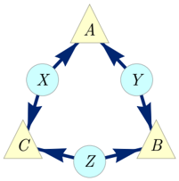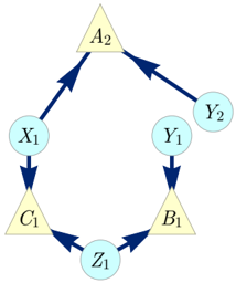Independently of Bell's work, Pearl later derived the instrumental inequality [31], which provides a necessary condition for the compatibility of a distribution with a causal structure known as the instrumental scenario . This causal structure comes up when considering, for instance, certain kinds of noncompliance in drug trials. More recently, Steudel and Ay [32] derived an inequality which must hold whenever a distribution on n variables is compatible with a causal structure where no set of more than c variables has a common ancestor, for arbitrary n, c ∈ N . More recent work has focused specifically on the simplest nontrivial case, with n = 3 and c = 2, a causal structure that has been called the Triangle scenario [21, 33] (Fig. 1). Recently, Henson, Lal and Pusey [22] have investigated those causal structures for which merely confirming that a given distribution on observed variables satisfies all of the conditional independence relations implied by d -separation relations does not guarantee that this distribution is compatible with the causal structure. They coined the term interesting for causal structures that have this property. They presented a catalogue of all potentially interesting causal structures having six or fewer nodes in [22, App. E], of which all but three were shown to be indeed interesting. Evans has also sought to generate such a catalogue [34]. The Bell scenario, the Instrumental scenario, and the Triangle 1 As illustrated by the vast amount of literature on the subject, the problem can still be difficult in practice, for example due to a large number of variables in certain applications or due to finite statistics. 2 The cardinality of a variable is the number of possible values it can take. 3 Techniques for finding approximate solutions to nonlinear quantifier elimination may help [9]. 4 The current article being another example of the phenomenon [9, 23-30]. scenario all appear in the catalogue, together with many others. Furthermore,they provided numerical evidence and an intuitive argument in favour of the hypothesis that the fraction of causal structures that are interesting increases as the total number of nodes increases. This highlights the need for moving beyond a case-by-case consideration of individual causal structures and for developing techniques for deriving constraints beyond conditional independence relations that can be applied to any interesting causal structure. Shannon-type entropic inequalities are an example of such constraints [21, 25, 32, 33, 35]. They can be derived for a given causal structure with relative ease, via exclusively linear quantifier elimination, since conditional independence relations are linear equations at the level of entropies. They also have the advantage that they apply for any finite cardinality of the observed variables. Recent work has also looked at non-Shannon type inequalities, potentially further strengthening the entropic constraints [26, 36]. However, entropic techniques are still wanting, since the resulting inequalities are often rather weak. For example, they are not sensitive enough to witness some known incompatibilities, in particular for distributions that only arise in quantum but not classical models with a given causal structure [21, 26] 5 . In order to improve this state of affairs, we here introduce a new technique for deriving necessary conditions for the compatibility of a distribution of observed variables with a given causal structure, which we term the inflation technique . This technique is frequently capable of witnessing incompatibility when many other causal inference techniques fail. For example, in Example 2 of Sec. III B we prove that the tripartite 'W-type' distribution is incompatible with the Triangle scenario, despite the incompatibility being invisible to other causal inference tools such as conditional independence relations, Shannon-type [25, 33, 35] or non-Shanon-type entropic inequalities [26], or covariance matrices [27]. The inflation technique works roughly as follows. For a given causal structure under consideration, one can construct many new causal structures, termed inflations of this causal structure. An inflation duplicates one or more of the nodes of the original causal structure, while mirroring the form of the subgraph describing each node's ancestry. Furthermore, the causal parameters that one adds to the inflated causal structure mirror those of the original causal structure. We show that if marginal distributions on certain subsets of the observed variables in the original causal structure are compatible with the original causal structure, then the same marginal distributions on certain copies of those subsets in the inflated causal structure are compatible with the inflated causal structure (Lemma 4). Similarly, we show that any necessary condition for compatibility of such distributions with the inflated causal structure translates into a necessary condition for compatibility with the original causal structure (Corollary 6). Thus, applying standard techniques for deriving causal compatibility inequalities to the inflated causal structure typically results in new causal compatibility inequalities for the original causal structure. The reader interested in seeing an example of how our technique works may want to take a sneak peak at Sec. III B. Concretely, we consider causal compatibility inequalities for the inflated causal structure that are obtained as follows. One begins by identifying inequalities for the marginal problem , which is the problem of determining when a given family of marginal distributions on some subsets of variables can arise as marginals of a global joint distribution. One then looks for sets of variables within the inflated causal structure which admit of nontrivial d-separation relations . (We mainly consider sets of variables with disjoint ancestries.) For each such set, one writes down the appropriate factorization of their joint distribution. These factorization conditions are finally substituted into the marginal problem inequalities to obtain causal compatibility inequalities for the inflated causal structure. Although these constraints are extremely weak, the inflation technique turns them into powerful necessary conditions for compatibility with the original causal structure. We show how to identify all relevant factorization conditions from the structure of the inflated causal structure, and also how to obtain all marginal problem inequalities by enumerating all facets of the associated marginal polytope (Sec. IV B). Translating the resulting causal compatibility inequalities on the inflated causal structure back to the original causal structure, we obtain causal compatibility conditions in the form of nonlinear (polynomial) inequalities. As a concrete example of our technique, we present all the causal compatibility inequalities that can be derived in this manner from a particular inflation of the Triangle scenario (Sec. IV C). In general, we also show how to efficiently obtain a partial set of marginal problem inequalities by enumerating transversals of a certain hypergraph (Sec. IV D). Besides the entropic techniques discussed above, our method is the first systematic tool for causal inference with latent variables that goes beyond observed conditional independence relations while not assuming any bounds on the cardinality of each latent variable. While our method can be used to systematically generate necessary conditions for compatibility with a given causal structure, we do not know whether the set of inequalities thus generated are also sufficient. 5 It should be noted that non-standard entropic inequalities can be obtained through a fine-graining of the causal scenario, namely by conditioning on the distinct finite possible outcomes of root variables ('settings'), and these types of inequalities have proven somewhat sensitive to quantum-classical separations [33, 37, 38]. Such inequalities are still limited, however, in that they are only applicable to those causal structures which feature observed root nodes. The potential utility of entropic analysis where fine-graining is generalized to non -root observed nodes is currently being explored by E.W. and Rafael Chaves. Jacques Pienaar has also alluded to similar considerations as a possible avenue for further research [36]. We present our technique primarily as a tool for standard causal inference, but we also briefly discuss applications to quantum causal models [22, 23, 39-43] and causal models within generalized probabilistic theories [22] (Sec. V D). In particular, we discuss when our inequalities are necessary conditions for a distribution of observed variables to be compatible with a given causal structure within any generalized probabilistic theory [44, 45] rather than simply within classical probability theory. ## II. BASIC DEFINITIONS OF CAUSAL MODELS AND COMPATIBILITY A causal model consists of a pair of objects: a causal structure and a family of causal parameters . We define each in turn. First, recall that a directed acyclic graph (DAG) G consists of a finite set of nodes Nodes ( G ) and a set of directed edges Edges ( G ) ⊆ Nodes ( G ) × Nodes ( G ), meaning that an edge is an ordered pair of nodes, such that this directed graph is acylic , which means that there is no way to start and end at the same node by traversing edges forward. In the context of a causal model, each node X ∈ Nodes ( G ) will be equipped with a random variable that we denote by the same letter X . A directed edge X → Y corresponds to the possibility of a direct causal influence from the variable X to the variable Y . In this way, the edges represent causal relations. Our terminology for the causal relations between the nodes in a DAG is the standard one. The parents of a node X in G are defined as those nodes from which an outgoing edge terminates at X , i.e. Pa G ( X ) = { Y | Y → X } . When the graph G is clear from the context, we omit the subscript. Similarly, the children of a node X are defined as those nodes at which edges originating at X terminate, i.e. Ch G ( X ) = { Y | X → Y } . If X is a set of nodes, then we put Pa G ( X ) := ⋃ X ∈ X Pa G ( X ) and Ch G ( X ) := ⋃ X ∈ X Ch G ( X ). The ancestors of a set of nodes X , denoted An G ( X ), are defined as those nodes which have a directed path to some node in X , including the nodes in X themselves 6 . Equivalently, An ( X ) := ⋃ n ∈ N Pa n ( X ), where Pa n ( X ) is defined inductively via Pa 0 ( X ) := X and Pa n +1 ( X ) := Pa ( Pa n ( X )). A causal structure is a DAG that incorporates a distinction between two types of nodes: the set of observed nodes, and the set of latent nodes 7 . Following [22], we will depict the observed nodes by triangles and the latent nodes by circles, as in Fig. 1 8 . Henceforth, we will use G to refer to the causal structure rather than just the DAG, so that G includes a specification of which variables are observed, denoted ObservedNodes ( G ), and which are latent, denoted LatentNodes ( G ). Frequently, we will also imagine the causal structure to include a specification of the cardinalities of the observed variables. While these are finite in all of our examples, the inflation technique may apply in the case of continuous variables as well. Although we will not do so in this work, the inflation technique can also be applied in the presence of other types of constraints, e.g. when all variables are assumed to be Gaussian. The second component of a causal model is a family of causal parameters . The causal parameters specify, for each node X , the conditional probability distribution over the values of the random variable X , given the values of the variables in Pa ( X ). In the case of root nodes, we have Pa ( X ) = ∅ , and the conditional distribution is an unconditioned distribution. We write P Y | X for the conditional distribution of a variable Y given a variable X , while the particular conditional probability of the variable Y taking the value y given that the variable X takes the values x is denoted 9 P Y | X ( y | x ). Therefore, a family of causal parameters has the form $$\{ P _ { X | \text {$\mathbb{ }P_{G}(X)$} } \colon X \in \text {Nodes} ( G ) \} .$$ Finally, a causal model M consists of a causal structure together with a family of causal parameters, M = ( G, { P X | Pa G ( X ) : X ∈ Nodes ( G ) } ) . A causal model specifies a joint distribution of all variables in the causal structure via $$P _ { \text {Nodes} ( G ) } = \prod _ { X \in \text {Nodes} ( G ) } P _ { X | \text {Pa} _ { G } ( X ) } ,$$ where ∏ denotes the usual product of functions, so that e.g. ( P Y | X × P Y )( x, y ) = P Y | X ( y | x ) P X ( x ). A distribution P Nodes ( G ) arises in this way if and only if it satisfies the Markov conditions associated to G [1, Sec. 1.2]. 6 The inclusion of a node itself within the set of its ancestors is contrary to the colloquial use of the term 'ancestors'. One uses this definition so that any correlation between two variables can always be attributed to a common 'ancestor'. This includes, for instance, the case where one variable is a parent of the other. 7 Pearl [1, Def. 2.3.2] uses the term latent structure when referring to a DAG supplemented by a specification of latent nodes, whereas here that specification is implicit in our term causal structure . 8 Note that this convention differs from that of [39], where triangles represent classical variables and circles represent quantum systems. 9 Although our notation suggests that all variables are either discrete or described by densities, we do not make this assumption. All of our equations can be translated straightforwardly into proper measure-theoretic notation. The joint distribution of the observed variables is obtained from the joint distribution of all variables by marginalization over the latent variables, $$P _ { \text {ObservedNodes} ( G ) } = \sum _ { \{ U \colon U \in \text {LatentNodes} ( G ) \} } P _ { \text {Nodes} ( G ) } ,$$ where ∑ U denotes marginalization over the (latent) variable U , so that ( ∑ U P UV )( v ) := ∑ u P UV ( uv ). Definition 1. A given distribution P ObservedNodes ( G ) is compatible with a given causal structure G if there is some choice of the causal parameters that yields P ObservedNodes ( G ) via Eqs. (2,3). A given family of distributions on a family of subsets of observed variables is compatible with a given causal structure if and only if there exists some P ObservedNodes ( G ) such that both 1. P ObservedNodes ( G ) is compatible with the causal structure, and 2. P ObservedNodes ( G ) yields the given family as marginals. ## III. THE INFLATION TECHNIQUE FOR CAUSAL INFERENCE ## A. Inflations of a Causal Model We now introduce the notion of an inflation of a causal model . If a causal model specifies a causal structure G , then an inflation of this model specifies a new causal structure, G ′ , which we refer to as an inflation of G . For a given causal structure G , there are many causal structures G ′ constituting an inflation of G . We denote the set of such causal structures Inflations ( G ). The particular choice of G ′ ∈ Inflations ( G ) then determines how to map a causal model M on G into a causal model M ′ on G ′ , since the family of causal parameters of M ′ will be determined by a function M ′ = Inflation G → G ′ ( M ) that we define below. We begin by defining when a causal structure G ′ is an inflation of G , building on some preliminary definitions. For any subset of nodes X ⊆ Nodes ( G ), we denote the induced subgraph on X by SubDAG G ( X ). It consists of the nodes X and those edges of G which have both endpoints in X . Of special importance to us is the ancestral subgraph AnSubDAG G ( X ), which is the subgraph induced by the ancestry of X , AnSubDAG G ( X ) := SubDAG G ( An G ( X )). In an inflated causal structure G ′ , every node is also labelled by a node of G . That is, every node of the inflated causal structure G ′ is a copy of some node of the original causal structure G , and the copies of a node X of G in G ′ are denoted X 1 , . . . , X k . The subscript that indexes the copies is termed the copy-index . A copy is classified as observed or latent according to the classification of the original. Similarly, any constraints on cardinality or other types of constraints such as Gaussianity are also inherited from the original. When two objects (e.g. nodes, sets of nodes, causal structures, etc. . . ) are the same up to copy-indices, then we use ∼ to indicate this, as in X i ∼ X j ∼ X . In particular, X ∼ X ′ for sets of nodes X ⊆ Nodes ( G ) and X ′ ⊆ Nodes ( G ′ ) if and only if X ′ contains exactly one copy of every node in X . Similarly, SubDAG G ′ ( X ′ ) ∼ SubDAG G ( X ) means that in addition to X ∼ X ′ , an edge is present between two nodes in X ′ if and only if it is present between the two associated nodes in X . In order to be an inflation, G ′ must locally mirror the causal structure of G : Definition 2. The causal structure G ′ is said to be an inflation of G , that is, G ′ ∈ Inflations ( G ) , if and only if for every V i ∈ ObservedNodes ( G ′ ) , the ancestral subgraph of V i in G ′ is equivalent, under removal of the copy-index, to the ancestral subgraph of V in G , $$G ^ { \prime } \in \text {Inflations} ( G ) \quad \text {iff} \quad \forall V _ { i } \in \text {ObservedNodes} ( G ^ { \prime } ) \colon \, A n \text {SubDAG} _ { G ^ { \prime } } ( V _ { i } ) \sim \text {AnSubDAG} _ { G } ( V ) .$$ Equivalently, the condition can be restated wholly in terms of local causal relationships, i.e. $$G ^ { \prime } \in \text {Inflations} ( G ) \quad \text {iff} \quad \forall X _ { i } \in \text {Nodes} ( G ^ { \prime } ) \colon \, \text {Pa} _ { G ^ { \prime } } ( X _ { i } ) \sim \text {Pa} _ { G } ( X ) .$$ In particular, this means that an inflation is a fibration of graphs [46], although there are fibrations that are not inflations. To illustrate the notion of inflation, we consider the causal structure of Fig. 1, which is called the Triangle scenario (for obvious reasons) and which has been studied recently by a number of authors [22 (Fig. E#8), 19 (Fig. 18b), 21 (Fig. 3), 33 (Fig. 6a), 40 (Fig. 1a), 47 (Fig. 8), 32 (Fig. 1b), 25 (Fig. 4b)]. Different inflations of the Triangle scenario are depicted in Figs. 2 to 6, which will be referred to as the Web , Spiral , Capped , and Cut inflation, respectively. We now define the function Inflation G → G ′ , that is, we specify how causal parameters are defined for a given inflated causal structure in terms of causal parameters on the original causal structure. <details> <summary>Image 1 Details</summary>  ### Visual Description ## Diagram: Triangular Node Network with Cyclic Flow ### Overview The image depicts a triangular network diagram with three primary nodes (A, B, C) arranged in a triangular formation. Each primary node connects to a secondary node (X, Y, Z) via directed arrows, forming a closed loop. The diagram uses color coding (yellow for primary nodes, light blue for secondary nodes) and directional arrows to indicate relationships. ### Components/Axes - **Nodes**: - **Primary Nodes**: - A (top position, yellow triangle) - B (bottom-right, yellow triangle) - C (bottom-left, yellow triangle) - **Secondary Nodes**: - X (left-center, light blue circle) - Y (right-center, light blue circle) - Z (bottom-center, light blue circle) - **Arrows**: - Blue directional arrows connect nodes in the following sequence: - A → X → C → Z → B → Y → A (forming a closed loop) - **Color Legend**: - Yellow: Primary nodes (A, B, C) - Light Blue: Secondary nodes (X, Y, Z) - Blue: Arrows (no explicit legend, inferred from visual context) ### Detailed Analysis 1. **Node Placement**: - Primary nodes (A, B, C) form an equilateral triangle. - Secondary nodes (X, Y, Z) are positioned between primary nodes: - X between A and C - Y between B and A - Z between C and B 2. **Flow Direction**: - Arrows create a cyclical path: A → X → C → Z → B → Y → A. - No bidirectional or divergent arrows; all connections are unidirectional. 3. **Color Coding**: - Primary nodes (yellow) are larger and more prominent. - Secondary nodes (light blue) are smaller and intermediate in the flow. ### Key Observations - The diagram emphasizes cyclical interdependence between primary and secondary nodes. - Secondary nodes act as intermediaries in the flow between primary nodes. - No explicit labels for arrows, but their direction is unambiguous from visual cues. - Symmetry in node placement suggests balanced relationships. ### Interpretation This diagram likely represents a **feedback loop** or **process flow** where: - Primary nodes (A, B, C) represent core entities (e.g., departments, systems, or stages). - Secondary nodes (X, Y, Z) symbolize transitional states, dependencies, or intermediate processes. - The cyclical arrow pattern implies continuous interaction, such as: - A data processing pipeline with feedback mechanisms. - Organizational workflows requiring cross-departmental collaboration. - A theoretical model of systemic interdependence (e.g., ecological or economic systems). The absence of numerical data or explicit labels for arrows suggests the diagram prioritizes structural relationships over quantitative metrics. The closed loop reinforces the idea of perpetual motion or recurring processes. </details> FIG. 1. The Triangle scenario. 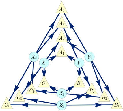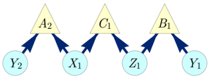FIG. 2. The Web inflation of the Triangle scenario where each latent node has been duplicated and each observed node has been quadrupled. The four copies of each observed node correspond to the four possible choices of parentage given the pair of copies of each latent parent of the observed node. <details> <summary>Image 2 Details</summary>  ### Visual Description ## Flowchart Diagram: System Architecture or Process Flow ### Overview The diagram depicts a hierarchical, layered structure with directional flow between nodes. It consists of six tiers of labeled nodes (A1-A4, B1-B4, C1-C4, X1-X2, Y1-Y2, Z1-Z2) connected by dark blue arrows. Nodes are color-coded: yellow (A), light blue (X/Y), dark blue (B/C), and cyan (Z). The flow progresses from top (A nodes) to bottom (Z nodes), suggesting a top-down process or data flow. ### Components/Axes - **Nodes**: - **Top Layer (A)**: A1-A4 (yellow triangles) - **Middle Layer (X/Y)**: X1-X2 (light blue circles), Y1-Y2 (light blue circles) - **Lower Middle Layer (B/C)**: B1-B4 (dark blue circles), C1-C4 (dark blue circles) - **Base Layer (Z)**: Z1-Z2 (cyan circles) - **Arrows**: Dark blue, unidirectional, connecting nodes between layers. - **Color Coding**: - Yellow (A nodes) → Light Blue (X/Y) → Dark Blue (B/C) → Cyan (Z) - No explicit legend, but color consistency implies categorical grouping. ### Detailed Analysis - **Top Layer (A)**: - A1-A4 form a pyramid structure. - Arrows from A1-A4 point to X1, X2, Y1, Y2 (middle layer). - **Middle Layer (X/Y)**: - X1-X2 and Y1-Y2 receive input from A nodes. - Arrows from X1-X2 and Y1-Y2 direct to B1-B4 and C1-C4 (lower middle layer). - **Lower Middle Layer (B/C)**: - B1-B4 and C1-C4 receive input from X/Y nodes. - Arrows from B1-B4 and C1-C4 point to Z1-Z2 (base layer). - **Base Layer (Z)**: - Z1-Z2 are terminal nodes with no outgoing arrows. - Z1 connects to B1-B4 and C1-C3; Z2 connects to B4 and C4. ### Key Observations 1. **Hierarchical Flow**: - Data/process flows from A (top) → X/Y → B/C → Z (bottom). 2. **Symmetry**: - Left and right sides mirror each other (e.g., A1→X1→B1→Z1; A4→Y2→B4→Z2). 3. **Terminal Nodes**: - Z1 and Z2 act as endpoints with no further connections. 4. **Missing Connections**: - No direct links between X/Y nodes or between B/C nodes. ### Interpretation This diagram likely represents a **system architecture** or **data flow process** with the following implications: - **Layered Dependency**: Higher-tier nodes (A) influence middle-tier nodes (X/Y), which in turn govern lower-tier nodes (B/C), culminating in foundational nodes (Z). - **Symmetry**: The mirrored structure suggests redundancy or parallel processing paths (e.g., X1 and X2 may handle similar roles on opposite sides). - **Terminal Nodes (Z)**: Z1 and Z2 could represent final outputs, storage, or decision points where the process concludes. - **Potential Gaps**: The absence of feedback loops or bidirectional arrows implies a strictly linear, non-iterative process. ### Uncertainties - **Purpose of Nodes**: Without context, the exact function of A/B/C/X/Y/Z nodes (e.g., data types, processes) remains speculative. - **Color Significance**: While colors group nodes, their semantic meaning (e.g., priority, category) is not explicitly defined. 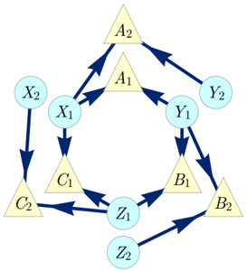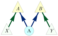</details> FIG. 3. The Spiral inflation of the Triangle scenario. Notably, this causal structure is the ancestral subgraph of the set { A 1 A 2 B 1 B 2 C 1 C 2 } in the Web inflation (Fig. 2). <details> <summary>Image 3 Details</summary>  ### Visual Description ## Diagram: Network Flowchart with Interconnected Components ### Overview The image depicts a directed graph (flowchart) illustrating relationships and flows between labeled nodes. Nodes are color-coded: yellow triangles (A1, A2, B1, B2, C1, C2) and blue circles (X1, X2, Y1, Y2, Z1, Z2). Arrows indicate bidirectional or unidirectional connections, forming cycles and hierarchical relationships. ### Components/Axes - **Nodes**: - **Yellow Triangles** (A1, A2, B1, B2, C1, C2): Likely represent primary components or categories. - **Blue Circles** (X1, X2, Y1, Y2, Z1, Z2): Likely represent secondary or intermediary nodes. - **Arrows**: - **Dark Blue Arrows**: Indicate directional relationships (e.g., A1 → X1, X1 → A1). - **Bidirectional Arrows**: Suggest mutual dependencies (e.g., A1 ↔ X1, Y1 ↔ B1). ### Detailed Analysis 1. **Central Cycle**: - A1 ↔ X1 ↔ C1 ↔ Z1 ↔ B1 ↔ Y1 ↔ A1 forms a central loop, indicating a core interdependent system. 2. **Peripheral Loops**: - A2 ↔ Y2, B2 ↔ Z2, and C2 ↔ X2 form smaller, isolated loops, suggesting modular subsystems. 3. **Directional Flow**: - Arrows from A1 to X1/Y1/A2 and vice versa imply bidirectional interactions. - Arrows from B1 to Y1/Z1 and vice versa reinforce mutual dependencies. - Arrows from C1 to X1/Z1 and vice versa highlight cross-connections. ### Key Observations - **Hub Nodes**: X1, Y1, Z1 act as central hubs, connecting multiple nodes and cycles. - **Modularity**: Subsystems (A2-Y2, B2-Z2, C2-X2) operate independently but are linked to the central cycle. - **Redundancy**: Bidirectional arrows suggest feedback loops or redundancy in the system. ### Interpretation The diagram represents a complex, interconnected system with modular subsystems and central hubs. The central cycle (A1-X1-C1-Z1-B1-Y1-A1) likely represents a core process with mutual dependencies, while peripheral loops (A2-Y2, B2-Z2, C2-X2) may denote self-sustaining or isolated components. The bidirectional arrows emphasize reciprocal relationships, suggesting feedback mechanisms or equilibrium states. This structure could model organizational workflows, data flow in a network, or interdependent processes in a technical system. The absence of numerical values implies the focus is on relational dynamics rather than quantitative metrics. </details> Definition 3. Consider causal models M and M ′ where DAG ( M ) = G and DAG ( M ′ ) = G ′ , where G ′ is an inflation of G . Then M ′ is said to be the G → G ′ inflation of M , that is, M ′ = Inflation G → G ′ ( M ) , if and only if for every node X i in G ′ , the manner in which X i depends causally on its parents within G ′ is the same as the manner in which X depends causally on its parents within G . Noting that X i ∼ X and that Pa G ′ ( X i ) ∼ Pa G ( X ) by Eq. (5) , one can formalize this condition as: $$\forall X _ { i } \in \text {Nodes} ( G ^ { \prime } ) \, \colon \, P _ { X _ { i } | \text {$p_{a}_{G^{\prime}}(X_{i})}$} = P _ { X | \text {$p_{a}_{G}(X)$} } .$$ For a given triple G , G ′ , and M , this definition specifies a unique inflation model M ′ , resulting in a well-defined function Inflation G → G ′ . To sum up, the inflation of a causal model is a new causal model where (i) each variable in the original causal structure may have counterparts in the inflated causal structure with ancestral subgraphs mirroring those of the <details> <summary>Image 4 Details</summary>  ### Visual Description ## Flowchart Diagram: System Process Flow ### Overview The image depicts a directed graph (flowchart) with labeled nodes and directional arrows. The diagram illustrates a process flow involving decision points (triangles) and data/process nodes (circles). Arrows indicate the direction of flow or dependency between components. ### Components/Axes - **Nodes**: - **Triangles** (likely decision points or actions): `A1`, `A2`, `B1`, `C1` - **Circles** (likely data/process nodes): `X1`, `Y1`, `Y2`, `Z1` - **Arrows**: Blue directional arrows connecting nodes, indicating flow or relationships. - **No explicit legend, axis titles, or scales** (typical for flowcharts). ### Detailed Analysis 1. **Node Connections**: - `A2` → `A1` and `A2` → `Y2` - `A1` → `X1` and `A1` → `Y1` - `Y1` → `B1` - `B1` → `Z1` - `Z1` → `C1` - `C1` → `A1` (feedback loop) - `X1` → `C1` 2. **Structure**: - **Top-level nodes**: `A2` (root) and `Y2` (terminal node). - **Central loop**: `A1` → `Y1` → `B1` → `Z1` → `C1` → `A1`. - **Parallel path**: `A1` → `X1` → `C1` (shortcut to the loop). 3. **Color Coding**: - Triangles: Light yellow (decision/action nodes). - Circles: Light blue (data/process nodes). - Arrows: Dark blue (flow direction). ### Key Observations - **Feedback Loop**: `C1` → `A1` creates a cyclical dependency, suggesting iterative processing. - **Divergence**: `A2` splits into two paths (`A1` and `Y2`), indicating branching logic. - **Convergence**: `X1` and `Z1` both feed into `C1`, merging data/process streams. - **Terminal Node**: `Y2` has no outgoing arrows, acting as an endpoint. ### Interpretation This flowchart represents a system with **modular decision-making** and **data flow**. The feedback loop between `A1` and `C1` implies a recurring process (e.g., validation, iteration). The divergence at `A2` suggests conditional branching (e.g., `A2` determines whether to proceed via `A1` or terminate at `Y2`). The convergence at `C1` indicates integration of inputs from `X1` and `Z1`, which may represent parallel subsystems or data sources. The terminal node `Y2` could represent an exit condition or output. The diagram emphasizes **cyclic dependencies** and **modularity**, common in workflows like software pipelines, decision trees, or state machines. 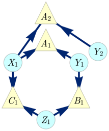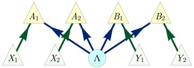</details> FIG. 4. The Capped inflation of the Triangle scenario; notably also the ancestral subgraph of the set { A 1 A 2 B 1 C 1 } in the Spiral inflation (Fig. 3). FIG. 5. The Cut inflation of the Triangle scenario; notably also the ancestral subgraph of the set { A 2 B 1 C 1 } in the Capped inflation (Fig. 4). Unlike the other examples, this inflation does not contain the Triangle scenario as a subgraph. <details> <summary>Image 5 Details</summary>  ### Visual Description ## Flowchart Diagram: Cyclic Process Flow ### Overview The image depicts a cyclic flowchart with seven nodes connected by directional arrows. The nodes alternate between triangular (A2, B1, C1) and circular (X1, Y1, Y2, Z1) shapes. Arrows indicate a unidirectional flow from one node to the next, forming a closed loop. Colors are used to differentiate node types: yellow for triangles, light blue for circles, and dark blue for arrows. ### Components/Axes - **Nodes**: - Triangular: A2 (top), B1 (bottom-right), C1 (bottom-left) - Circular: X1 (left), Y1 (bottom-right), Y2 (top-right), Z1 (bottom-center) - **Arrows**: Dark blue, unidirectional, connecting nodes in sequence. - **No explicit legend**: Colors are descriptive but not formally labeled. - **No axes or scales**: Diagram focuses on logical flow rather than quantitative data. ### Detailed Analysis 1. **Flow Sequence**: - A2 → X1 → C1 → Z1 → B1 → Y1 → Y2 → A2 - Forms a closed loop with no branching or termination points. 2. **Node Relationships**: - Triangular nodes (A2, B1, C1) act as decision points or process stages. - Circular nodes (X1, Y1, Y2, Z1) represent data inputs, outputs, or intermediate states. 3. **Color Coding**: - Yellow triangles (A2, B1, C1) may signify critical stages or decision nodes. - Light blue circles (X1, Y1, Y2, Z1) likely denote data or resource nodes. - Dark blue arrows emphasize directional flow. ### Key Observations - **Cyclic Nature**: The loop suggests a repeating process (e.g., workflow, data pipeline, or feedback system). - **Symmetry**: The arrangement of nodes creates a balanced, hexagonal-like structure. - **No Outliers**: All nodes are equally connected; no node is isolated or bypassed. ### Interpretation This diagram likely represents a **closed-loop system** where each node contributes to a continuous cycle. For example: - **A2** could initiate a process (e.g., data collection). - **X1, Y1, Y2, Z1** might represent data transformations or resource allocations. - **B1 and C1** could act as decision gates or validation steps before returning to A2. The absence of a legend or numerical data implies the focus is on **logical flow** rather than quantitative analysis. The symmetry and uniformity suggest a designed, intentional process with no inherent inefficiencies or bottlenecks. Further context (e.g., labels for nodes) would clarify the specific application (e.g., business workflow, scientific experiment, or software architecture). </details> FIG. 6. A different depiction of the Cut inflation of Fig. 5. <details> <summary>Image 6 Details</summary>  ### Visual Description ## Flowchart Diagram: Decision Process with Multiple Outcomes ### Overview The image depicts a flowchart with three decision nodes (triangles) and four outcome nodes (circles). Arrows indicate directional relationships between nodes, suggesting a process flow from decisions to outcomes. The diagram uses color coding: yellow for decision nodes and light blue for outcome nodes. ### Components/Axes - **Decision Nodes (Triangles)**: - **A2**: Positioned at the top-left, connected via two arrows to outcome nodes. - **C1**: Centered, connected via one arrow to an outcome node. - **B1**: Top-right, connected via one arrow to an outcome node. - **Outcome Nodes (Circles)**: - **Y2**: Bottom-left, connected from A2. - **X1**: Middle-left, connected from A2. - **Z1**: Middle-right, connected from C1. - **Y1**: Bottom-right, connected from B1. - **Arrows**: Dark blue, indicating flow direction. No legends or axis titles are present. ### Detailed Analysis - **Node Connections**: - **A2** → **Y2** (leftward arrow) and **A2** → **X1** (rightward arrow). - **C1** → **Z1** (rightward arrow). - **B1** → **Y1** (rightward arrow). - **Spatial Layout**: - Decision nodes are arranged horizontally at the top. - Outcome nodes are positioned below their respective decision nodes, with **Y2** and **X1** aligned left, **Z1** centered, and **Y1** right. ### Key Observations 1. **Branching Structure**: **A2** splits into two outcomes (**Y2**, **X1**), while **C1** and **B1** each lead to a single outcome. 2. **Repetition**: The outcome node **Y1** shares its label with **Y2**, suggesting potential equivalence or redundancy in outcomes. 3. **Simplicity**: No numerical values, scales, or additional annotations are present. ### Interpretation This flowchart likely represents a decision tree or process model where: - **A2** acts as a bifurcation point, leading to divergent outcomes (**Y2** and **X1**). - **C1** and **B1** represent linear decision paths with singular results (**Z1** and **Y1**). - The repetition of **Y1/Y2** may imply shared outcomes or a naming convention (e.g., "Y" as a category prefix). The diagram emphasizes structural relationships over quantitative data, focusing on logical flow rather than measurable trends. No anomalies or outliers are evident due to the absence of numerical data. </details> originals, and (ii) the manner in which a variable depends causally on its parents in the inflated causal structure is given by the manner in which its counterpart in the original causal structure depends causally on its parents. The operation of modifying a DAG and equipping the modified version with conditional probability distributions that mirror those of the original also appears in the do calculus and twin networks of Pearl [1], and moreover bears some resemblance to the adhesivity technique used in deriving non-Shannon-type entropic inequalities (see also Appendix E). We are now in a position to describe the key property of the inflation of a causal model, the one that makes it useful for causal inference. With notation as in Definition 3, let P X and P X ′ denote marginal distributions on some X ⊆ Nodes ( G ) and X ′ ⊆ Nodes ( G ′ ), respectively. Then $$\text {if} \quad X ^ { \prime } \sim X \text { and AnSubDAG_{G^{\prime}}(X)^{2} \sim AnSubDAG_{G}(X)} , \quad \text {then} \quad P _ { X ^ { \prime } } = P _ { X } .$$ This follows from the fact that the distributions on X ′ and X depend only on their ancestral subgraphs and the parameters defined thereon, which by the definition of inflation are the same for X ′ and for X . It is useful to have a name for those sets of observed nodes in G ′ which satisfy the antecedent of Eq. (7), that is, for which one can find a copy-index-equivalent set in the original causal structure G with a copy-index-equivalent ancestral subgraph. We call such subsets of the observed nodes of G ′ injectable sets , $$V ^ { \prime } & \in \text {InjectableSets} ( G ^ { \prime } ) \\ \text {iff} & \quad \exists V \subseteq \text {ObservedNodes} ( G ) \ \colon \ V ^ { \prime } \sim V \text { and AnSubDAG$_{G}$} ^ { \prime } ( V ^ { \prime } ) \sim \text {AnSubDAG} _ { G } ( V ) .$$ Similarly, those sets of observed nodes in the original causal structure G which satisfy the antecedent of Eq. (7), that is, for which one can find a corresponding set in the inflated causal structure G ′ with a copy-index-equivalent ancestral subgraph, we describe as images of the injectable sets under the dropping of copy-indices, $$V \in & \text {ImagesInjectableSets} ( G ) \\ \text {iff} \quad & \exists V ^ { \prime } \subseteq \text {ObservedNodes} ( G ^ { \prime } ) \ \colon \ V ^ { \prime } \sim V \text { and AnSubDAG$_{G}$} ^ { \prime } ( V ^ { \prime } ) \sim \text {AnSubDAG} _ { G } ( V ) .$$ Clearly, V ∈ ImagesInjectableSets ( G ) iff ∃ V ′ ⊆ InjectableSets ( G ′ ) such that V ∼ V ′ . For example in the Spiral inflation of the Triangle scenario depicted in Fig. 3, the set { A 1 B 1 C 1 } is injectable because its ancestral subgraph is equivalent up to copy-indices to the ancestral subgraph of { ABC } in the original causal structure, and the set { A 2 C 1 } is injectable because its ancestral subgraph is equivalent to that of { AC } in the original causal structure. A set of nodes in the inflated causal structure can only be injectable if it contains at most one copy of any node from the original causal structure. More strongly, it can only be injectable if its ancestral subgraph contains at most one copy of any observed or latent node from the original causal structure. Thus, in Fig. 3, { A 1 A 2 C 1 } is not injectable because it contains two copies of A , and { A 2 B 1 C 1 } is not injectable because its ancestral subgraph contains two copies of Y . We can now express Eq. (7) in the language of injectable sets, $$P _ { V ^ { \prime } } = P _ { V } \text {\quad if\, } V ^ { \prime } \sim V \text {\ and\ } V ^ { \prime } \in \text {InjectableSets} ( G ^ { \prime } ) .$$ In the example of Fig. 3, injectability of the sets { A 1 B 1 C 1 } and { A 2 C 1 } thus implies that the marginals on each of these are equal to the marginals on their counterparts, { ABC } and { AC } , in the original causal model, so that P A 1 B 1 C 1 = P ABC and P A 2 C 1 = P AC . ## B. Witnessing Incompatibility Finally, we can explain why inflation is relevant for deciding whether a distribution is compatible with a causal structure. For a distribution P ObservedNodes ( G ) to be compatible with G , there must be a causal model M that yields it. Per Definition 1, given a P ObservedNodes ( G ) compatible with G , the family of marginals of P ObservedNodes ( G ) on the images of the injectable sets of observed variables in G , { P V : V ∈ ImagesInjectableSets ( G ) } , are also said to be compatible with G . Looking at the inflation model M ′ = Inflation G → G ′ ( M ), Eq. (10) implies that the family of distributions on the injectable sets given by { P V ′ : V ′ ∈ InjectableSets ( G ′ ) } - where P V ′ = P V for V ′ ∼ V - is compatible with G ′ . The same considerations apply for any family of distributions such that each set of variables in the family corresponds to an injectable set (i.e., when the family of distributions is associated with an incomplete collection of injectable sets.) Formally, Lemma 4. Let the causal structure G ′ be an inflation of G . Let S ′ ⊆ InjectableSets ( G ′ ) be a collection of injectable sets, and let S ⊆ ImagesInjectableSets ( G ) be the images of this collection under the dropping of copy-indices. If a distribution P ObservedNodes ( G ) is compatible with G , then the family of distributions { P V : V ∈ S } is compatible with G per Definition 1. Furthermore the corresponding family of distributions { P V ′ : V ′ ∈ S ′ } , defined via P V ′ = P V for V ′ ∼ V , must be compatible with G ′ . We have thereby related a question about compatibility with the original causal structure to one about compatibility with the inflated causal structure. If one can show that the new compatibility question on G ′ is answered in the negative, then it follows that the original compatibility question on G is answered in the negative as well. Some simple examples serve to illustrate the idea. ## Example 1 Incompatibility of perfect three-way correlation with the Triangle scenario Consider the following causal inference problem. We are given a joint distribution of three binary variables, P ABC , where the marginal on each variable is uniform and the three are perfectly correlated, $$P _ { A B C } = \frac { [ 0 0 0 ] + [ 1 1 1 ] } { 2 } , \quad i . e . , \quad P _ { A B C } ( a b c ) = \begin{cases} \frac { 1 } { 2 } & \text {if $a=b=c$} , \\ 0 & \text {otherwise,} \end{cases}$$ and we would like to determine whether it is compatible with the Triangle scenario (Fig. 1). The notation [ abc ] in Eq. (11) is shorthand for the deterministic distribution where A , B , and C take the values a, b , and c respectively; in terms of the Kronecker delta, [ abc ] := δ A,a δ B,b δ C,c . Since there are no conditional independence relations among the observed variables in the Triangle scenario, there is no opportunity for ruling out the distribution on the grounds that it fails to satisfy the required conditional independences. To solve the causal inference problem, we consider the Cut inflation (Fig. 5). The injectable sets include { A 2 C 1 } and { B 1 C 1 } . Their images in the original causal structure are { AC } and { BC } , respectively. We will show that the distribution of Eq. (11) is not compatible with the Triangle scenario by demonstrating that the contrary assumption of compatibility implies a contradiction. If the distribution of Eq. (11) were compatible with the Triangle scenario, then so too would its pair of marginals on { AC } and { BC } , which are given by: $$P _ { A C } = P _ { B C } = \frac { [ 0 0 ] + [ 1 1 ] } { 2 } .$$ By Lemma 4, this compatibility assumption would entail that the marginals $$P _ { A _ { 2 } C _ { 1 } } = P _ { B _ { 1 } C _ { 1 } } = \frac { [ 0 0 ] + [ 1 1 ] } { 2 } & & ( 1 2 )$$ are compatible with the Cut inflation of the Triangle scenario. We now show that the latter compatibility cannot hold, thereby obtaining our contradiction. It suffices to note that (i) the only joint distribution that exhibits perfect correlation between A 2 and C 1 and between B 1 and C 1 also exhibits perfect correlation between A 2 and B 1 , and (ii) A 2 and B 1 have no common ancestor in the Cut inflation and hence must be marginally independent in any distribution that is compatible with it. We have therefore certified that the distribution P ABC of Eq. (11) is not compatible with the Triangle scenario, recovering a result originally proven by Steudel and Ay [32]. ## Example 2 Incompatibility of the W-type distribution with the Triangle scenario Consider another causal inference problem on the Triangle scenario, namely, that of determining whether the distribution $$P _ { A B C } = \frac { [ 1 0 0 ] + [ 0 1 0 ] + [ 0 0 1 ] } { 3 } , \quad i . e . , \quad P _ { A B C } ( a b c ) = \begin{cases} \frac { 1 } { 3 } & \text {if $a+b+c=1$,} \\ 0 & \text {otherwise.} \end{cases}$$ is compatible with it. We call this the W-type distribution 10 . To settle this compatibility question, we consider the Spiral inflation of the Triangle scenario (Fig. 3). The injectable sets in this case include { A 1 B 1 C 1 } , { A 2 C 1 } , { B 2 A 1 } , { C 2 B 1 } , { A 2 } , { B 2 } and { C 2 } . 10 The name stems from the fact that this distribution is reminiscent of the famous quantum state appearing in [48], called the W state . Therefore, we turn our attention to determining whether the marginals of the W-type distribution on the images of these injectable sets are compatible with the Triangle scenario. These marginals are: $$P _ { A B C } = \frac { [ 1 0 0 ] + [ 0 1 0 ] + [ 0 0 1 ] } { 3 } ,$$ $$P _ { A C } = P _ { B A } = P _ { C B } = \frac { [ 1 0 ] + [ 0 1 ] + [ 0 0 ] } { 3 } ,$$ $$P _ { A } = P _ { B } = P _ { C } = \frac { 2 } { 3 } [ 0 ] + \frac { 1 } { 3 } [ 1 ] .$$ By Lemma 4, this compatibility holds only if the associated marginals for the injectable sets, namely, $$P _ { A _ { 1 } B _ { 1 } C _ { 1 } } = \frac { [ 1 0 0 ] + [ 0 1 0 ] + [ 0 0 1 ] } { 3 } ,$$ $$P _ { A _ { 2 } C _ { 1 } } = P _ { B _ { 2 } A _ { 1 } } = P _ { C _ { 2 } B _ { 1 } } = \frac { [ 1 0 ] + [ 0 1 ] + [ 0 0 ] } { 3 } ,$$ $$P _ { A _ { 2 } } = P _ { B _ { 2 } } = P _ { C _ { 2 } } = \frac { 2 } { 3 } [ 0 ] + \frac { 1 } { 3 } [ 1 ] , & & ( 1 9 )$$ are compatible with the Spiral inflation (Fig. 3). Eq. (18) implies that C 1 =0 whenever A 2 =1. It similarly implies that A 1 =0 whenever B 2 =1, and that B 1 =0 whenever C 2 =1, A =1 = ⇒ C =0 , $$B _ { 2 } = 1 \implies A _ { 1 } = 0 ,$$ $$C _ { 2 } { = } 1 \implies B _ { 1 } { = } 0 .$$ The Spiral inflation is such that A 2 , B 2 and C 2 have no common ancestor and consequently are marginally independent in any distribution compatible with it. Together with the fact that each value of these variables has a nonzero probability of occurrence (by Eq. (19)), this implies that $$\text {Sometimes } \ A _ { 2 } = & 1 \text { and } B _ { 2 } = & 1 \text { and } C _ { 2 } = & 1 .$$ Finally, Eq. (20) together with Eq. (21) entails $$\text {Sometimes} \quad A _ { 1 } = & 0 \text { and } B _ { 1 } = & 0 \text { and } C _ { 1 } = & 0 .$$ This, however, contradicts Eq. (17). Consequently, the family of marginals described in Eqs. (17-19) is not compatible with the causal structure of Fig. 3. By Lemma 4, this implies that the family of marginals described in Eqs. (14-16)-and therefore the W-type distribution of which they are marginals-is not compatible with the Triangle scenario. To our knowledge, this is a new result. In fact, the incompatibility of the W-type distribution with the Triangle scenario cannot be derived via any of the existing causal inference techniques. In particular: 1. Checking conditional independence relations is not relevant here, as there are no conditional independence relations between any observed variables in the Triangle scenario. 2. The relevant Shannon-type entropic inequalities for the Triangle scenario have been classified, and they do not witness the incompatibility [25, 33, 35]. 3. Moreover, no entropic inequality can witness the W-type distribution as unrealizable. Weilenmann and Colbeck [26] have constructed an inner approximation to the entropic cone of the Triangle causal structure, and the entropies of the W-distribution form a point in this cone. In other words, a distribution with the same entropic profile as the W-type distribution can arise from the Triangle scenario. 4. The newly-developed method of covariance matrix causal inference due to Kela et al. [27], which gives tighter constraints than entropic inequalities for the Triangle scenario, also cannot detect the incompatibility. Therefore, in this case at least, the inflation technique appears to be more powerful. We have arrived at our incompatibility verdict by combining inflation with reasoning reminiscent of Hardy's version of Bell's theorem [49, 50]. Sec. IV D will present a generalization of this kind of argument and its applications to causal inference. ## Example 3 Incompatibility of PR-box correlations with the Bell scenario Bell's theorem [17, 18, 20, 51] concerns the question of whether the distribution obtained in an experiment involving a pair of systems that are measured at space-like separation is compatible with a causal structure of the form of Fig. 7. Here, the observed variables are { A,B,X,Y } , and Λ is a latent variable acting as a common cause of A and B . We shall term this causal structure the Bell scenario . While the causal inference formulation of Bell's theorem is not the traditional one, several recent articles have introduced and advocated this perspective [19 (Fig. 19), 22 (Fig. E#2), 23 (Fig. 1), 33 (Fig. 1), 52 (Fig. 2b), 53 (Fig. 2)]. FIG. 7. The Bell scenario causal structure. The local outcomes, A and B , of a pair of measurements are assumed to each be a function of some latent common cause and their independent local experimental settings, X and Y . <details> <summary>Image 7 Details</summary>  ### Visual Description ## Diagram: Interconnected System Components ### Overview The diagram illustrates a network of four triangular components (A, B, X, Y) and a central circular node (Λ), connected by directional and bidirectional arrows. Arrows are color-coded (blue and green) to indicate different types of relationships or flows between elements. ### Components/Axes - **Nodes**: - **A**: Yellow triangle (top-left) - **B**: Yellow triangle (top-right) - **X**: Green triangle (bottom-left) - **Y**: Green triangle (bottom-right) - **Λ**: Blue circle (center) - **Arrows**: - **Blue arrows**: - From A to X (top-left to bottom-left) - From A to Y (top-left to bottom-right) - From B to X (top-right to bottom-left) - From B to Y (top-right to bottom-right) - Bidirectional between A and B (top-center) - **Green arrows**: - From X to A (bottom-left to top-left) - From Y to B (bottom-right to top-right) ### Detailed Analysis - **Directional Flow**: - Blue arrows indicate unidirectional influence from A and B to X and Y. - Green arrows suggest feedback loops from X and Y back to A and B. - The bidirectional blue arrow between A and B implies mutual interaction or dependency. - **Color Coding**: - Blue arrows dominate the network, emphasizing primary directional relationships. - Green arrows are limited to feedback paths, suggesting secondary or reactive interactions. ### Key Observations 1. **Central Node (Λ)**: Positioned at the center but lacks direct connections, potentially acting as a mediator or hub. 2. **Mutual Dependency**: A and B share a bidirectional relationship, indicating interdependence. 3. **Asymmetric Feedback**: Feedback loops (green arrows) only exist from X/Y to A/B, not vice versa. ### Interpretation This diagram likely represents a system where: - **A and B** are primary drivers or sources influencing **X and Y**. - **X and Y** provide feedback to refine or adjust A and B’s outputs. - The central node **Λ** may symbolize a shared resource, control mechanism, or balancing factor not directly involved in active flows. - The absence of feedback from X/Y to Λ suggests Λ’s role is passive or observational in this context. The structure resembles a **feedback control system** or **dependency graph**, where A and B regulate X and Y while receiving corrective input from them. The bidirectional link between A and B could represent collaborative or conflicting objectives requiring synchronization. </details> FIG. 8. An inflation of the Bell scenario causal structure, where both local settings and outcome variables have been duplicated. <details> <summary>Image 8 Details</summary>  ### Visual Description ## Flowchart Diagram: System Interaction Model ### Overview The diagram illustrates a hierarchical system with a central node (Λ) connected to four intermediate nodes (A1, A2, B1, B2), which in turn connect to terminal nodes (X1, X2, Y1, Y2). Arrows indicate directional relationships, with color-coded distinctions between direct and indirect influences. ### Components/Axes - **Nodes**: - Central node: Λ (light blue circle) - Intermediate nodes: A1, A2, B1, B2 (yellow triangles) - Terminal nodes: X1, X2, Y1, Y2 (gray triangles) - **Arrows**: - Green arrows: Labeled "Direct Influence" in legend - Blue arrows: Labeled "Indirect Influence" in legend - **Legend**: Positioned at bottom-right corner, explicitly mapping colors to influence types. ### Detailed Analysis 1. **Central Node (Λ)**: - Receives **blue arrows** (indirect influence) from A1, A2, B1, and B2. - Distributes **blue arrows** (indirect influence) to A1, A2, B1, and B2. 2. **Intermediate Nodes**: - **A1/A2**: - Receive blue arrows from Λ (indirect influence). - Distribute green arrows (direct influence) to X1 and X2, respectively. - **B1/B2**: - Receive blue arrows from Λ (indirect influence). - Distribute green arrows (direct influence) to Y1 and Y2, respectively. 3. **Terminal Nodes**: - X1, X2: Receive green arrows from A1 and A2 (direct influence). - Y1, Y2: Receive green arrows from B1 and B2 (direct influence). ### Key Observations - **Color Consistency**: All green arrows align with the "Direct Influence" legend label; blue arrows match "Indirect Influence." - **Flow Direction**: - Λ acts as a hub, mediating interactions between intermediate and terminal nodes. - No feedback loops or bidirectional relationships are depicted. - **Symmetry**: The diagram is balanced, with A1/A2/X1/X2 and B1/B2/Y1/Y2 forming mirrored subgraphs. ### Interpretation The diagram represents a **two-path influence model** where: 1. **Λ** serves as a central coordinator, indirectly affecting all terminal nodes through intermediate nodes (A1/A2/B1/B2). 2. **Direct Influence** (green arrows) originates exclusively from intermediate nodes to terminal nodes, suggesting localized control or decision-making at the A/B level. 3. **Indirect Influence** (blue arrows) flows bidirectionally between Λ and intermediate nodes, implying Λ’s role in modulating or regulating the system’s behavior without direct intervention at the terminal level. This structure could model organizational hierarchies, neural networks, or decision-making frameworks where central authority (Λ) delegates influence through intermediary layers (A/B nodes) to execute localized actions (X/Y nodes). The absence of feedback loops suggests a linear, top-down operational model. </details> We consider the distribution P ABXY = P AB | XY P X P Y , where P X and P Y are arbitrary full-support distributions on { 0 , 1 } 11 , and $$P _ { A B | X Y } = \begin{cases} \frac { 1 } { 2 } ( [ 0 0 ] + [ 1 1 ] ) & \text {if $x=0,y=0$} \\ \frac { 1 } { 2 } ( [ 0 0 ] + [ 1 1 ] ) & \text {if $x=1,y=0$} \\ \frac { 1 } { 2 } ( [ 0 0 ] + [ 1 1 ] ) & \text {if $x=0,y=1$} \\ \frac { 1 } { 2 } ( [ 0 1 ] + [ 1 0 ] ) & \text {if $x=1,y=1$} \end{cases} , \quad i . e . , \ P _ { A B | X Y } ( a b | x y ) = \begin{cases} \frac { 1 } { 2 } & \text {if $a\oplus b=x\cdoty$,} \\ 0 & \text {otherwise.} \end{cases}$$ This conditional distribution was discovered by Tsirelson [54] and later independently by Popescu and Rohrlich [55, 56]. It has become known in the field of quantum foundations as the PR-box after the latter authors. 12 The Bell scenario implies nontrivial conditional independences 13 among the observed variables, namely, X ⊥ ⊥ Y , A ⊥ ⊥ Y | X , and B ⊥ ⊥ X | Y , as well as those that can be generated from these by the semi-graphoid axioms [19]. It is straightforward to check that these conditional independence relations are respected by the P ABXY resulting from Eq. (23). It is well-known that this distribution is nonetheless incompatible with the Bell scenario, since it violates the CHSH inequality. Here we present a proof of incompatibility in the style of Hardy's proof of Bell's theorem [49] in terms of the inflation technique, using the inflation of the Bell scenario depicted in Fig. 8. We begin by noting that { A 1 B 1 X 1 Y 1 } , { A 2 B 1 X 2 Y 1 } , { A 1 B 2 X 1 Y 2 } , { A 2 B 2 X 2 Y 2 } , { X 1 } , { X 2 } , { Y 1 } , and { Y 2 } are all injectable sets. By Lemma 4, it follows that any causal model that recovers P ABXY inflates to a model that results in marginals $$P _ { A _ { 1 } B _ { 1 } X _ { 1 } Y _ { 1 } } = P _ { A _ { 2 } B _ { 1 } X _ { 2 } Y _ { 1 } } = P _ { A _ { 1 } B _ { 2 } X _ { 1 } Y _ { 2 } } = P _ { A _ { 2 } B _ { 2 } X _ { 2 } Y _ { 2 } } = P _ { A B X Y } ,$$ $$P _ { X _ { 1 } } = P _ { X _ { 2 } } = P _ { X } , \quad P _ { Y _ { 1 } } = P _ { Y _ { 2 } } = P _ { Y } .$$ Using the definition of conditional probability, we infer that $$P _ { A _ { 1 } B _ { 1 } | X _ { 1 } Y _ { 1 } } = P _ { A _ { 2 } B _ { 1 } | X _ { 2 } Y _ { 1 } } = P _ { A _ { 1 } B _ { 2 } | X _ { 1 } Y _ { 2 } } = P _ { A _ { 2 } B _ { 2 } | X _ { 2 } Y _ { 2 } } = P _ { A B | X Y } .$$ Because { X 1 } , { X 2 } , { Y 1 } , and { Y 2 } have no common ancestor in the inflated causal structure, these variables must be marginally independent in any distribution compatible with it, so that P X 1 X 2 Y 1 Y 2 = P X 1 P X 2 P Y 1 P Y 2 . Given the assumption that the distributions P X and P Y have full support, it follows from Eq. (25) that Sometimes X = 0 and X = 1 and Y = 0 and Y = 1 . $$\text {Sometimes} \quad X _ { 1 } = 0 \, \text { and } \, X _ { 2 } = 1 \, \text { and } \, Y _ { 1 } = 0 \, \text { and } \, Y _ { 2 } = 1 .$$ 11 In the literature on the Bell scenario, the variables X and Y are termed 'settings'. Generally, we may think of observed root variables as settings, coloring them light green in the figures. They are natural candidates for variables to condition on. 12 The PR-box is of interest because it represents a manner in which experimental observations could deviate from the predictions of quantum theory while still being consistent with relativity. 13 Recall that variables X and Y are conditionally independent given Z if P XY | Z ( xy | z ) = P X | Z ( x | z ) P Y | Z ( y | z ) for all z with P Z ( z ) > 0. Such a conditional independence is denoted by X ⊥ ⊥ Y | Z . On the other hand, from Eq. (26) together with the definition of PR-box, Eq. (23), we conclude that $$\begin{array} { l c r } X _ { 1 } = & 0 , \, Y _ { 1 } = & 0 & \Longrightarrow & A _ { 1 } = B _ { 1 } , \\ X _ { 1 } = & 0 , \, Y _ { 2 } = & 1 & \Longrightarrow & A _ { 1 } = B _ { 2 } , \\ X _ { 2 } = & 1 , \, Y _ { 1 } = & 0 & \Longrightarrow & A _ { 2 } = B _ { 1 } , \\ X _ { 2 } = & 1 , \, Y _ { 2 } = & 1 & \Longrightarrow & A _ { 2 } \neq B _ { 2 } . \end{array}$$ Combining this with Eq. (27), we obtain $$\text {Sometimes} \quad A _ { 1 } = B _ { 1 } \text { and } A _ { 1 } = B _ { 2 } \text { and } A _ { 2 } = B _ { 1 } \text { and } A _ { 2 } \neq B _ { 2 } .$$ No values of A 1 , A 2 , B 1 , and B 2 can jointly satisfy these conditions. So we have reached a contradiction, showing that our original assumption of compatibility of P ABXY with the Bell scenario must have been false. The structure of this argument parallels that of standard proofs of the incompatibility of the PR-box with the Bell scenario. Standard proofs focus on a set of variables { A 0 A 1 B 0 B 1 } where A x is the value of A when X = x and B y is the value of B when Y = y . Note that the distribution ∑ Λ P A 0 | Λ P A 1 | Λ P B 0 | Λ P B 1 | Λ P Λ is a joint distribution of these four variables for which the marginals on pairs { A 0 B 0 } , { A 0 B 1 } , { A 1 B 0 } and { A 1 B 1 } are those that can arise in the Bell scenario. The existence of such a joint distribution rules out the possibility of having A 1 = B 1 , A 1 = B 2 , A 2 = B 1 but A 2 = B 2 , and therefore shows that the PR-box distribution is incompatible with the Bell scenario [57, 58]. In light of our use of Eq. (27), the reasoning based on the inflation of Fig. 8 is really the same argument in disguise. Appendix G shows that the inflation of the Bell scenario depicted in Fig. 8 is sufficient to witness the incompatibility of any distribution that is incompatible with the Bell scenario. ## C. Deriving Causal Compatibility Inequalities The inflation technique can be used not only to witness the incompatibility of a given distribution with a given causal structure, but also to derive necessary conditions that a distribution must satisfy to be compatible with the given causal structure. These conditions can always be expressed as inequalities, and we will refer to them as causal compatibility inequalities 14 . Formally, we have: Definition 5. Let G be a causal structure and let S be a family of subsets of the observed variables of G , S ⊆ 2 ObservedNodes ( G ) . Let I S denote an inequality that operates on the corresponding family of distributions, { P V : V ∈ S } . Then I S is a causal compatibility inequality for the causal structure G whenever it is satisfied by every family of distributions { P V : V ∈ S } that is compatible with G . While violation of a causal compatibility inequality witnesses the incompatibility with the causal structure, satisfaction of the inequality does not guarantee compatibility. This is the sense in which it merely provides a necessary condition for compatibility. The inflation technique is useful for deriving causal compatibility inequalities because of the following consequence of Lemma 4: Corollary 6. Suppose that G ′ is an inflation of G . Let S ′ ⊆ InjectableSets ( G ′ ) be a family of injectable sets and S ⊆ ImagesInjectableSets ( G ) the images of members of S ′ under the dropping of copy-indices. Let I S ′ be a causal compatibility inequality for G ′ operating on families { P V ′ : V ′ ∈ S ′ } . Define an inequality I S as follows: in the functional form of I S ′ , replace every occurrence of a term P V ′ by P V for the unique V ∈ S with V ∼ V ′ . Then I S is a causal compatibility inequality for G operating on families { P V : V ∈ S } . Proof. Suppose that the family { P V : V ∈ S } is compatible with G . By Lemma 4, it follows that the family { P V ′ : V ′ ∈ S ′ } where P V ′ := P V for V ′ ∼ V is compatible with G ′ . Since I S ′ is a causal compatibility inequality for G ′ , it follows that { P V ′ : V ′ ∈ S ′ } satisfies I S ′ . But by the definition of I S , its evaluation on { P V : V ∈ S } is equal to I S ′ evaluated on { P V ′ : V ′ ∈ S ′ } . It therefore follows that { P V : V ∈ S } satisfies I S . Since { P V : V ∈ S } was an arbitrary family compatible with G , we conclude that I S is a causal compatibility inequality for G . 14 Note that we can include equality constraints for causal compatibility within the framework of causal compatibility inequalities alone; it suffices to note that an equality constraint can always be expressed as a pair of inequalities, i.e. satisfying x = y is equivalent to satisfying both x ≤ y and x ≥ y . The requirement that a distribution must be Markov (or Nested Markov) relative to a DAG is usually formulated as a set of equality constraints. We now present some simple examples of causal compatibility inequalities for the Triangle scenario that one can derive from the inflation technique via Corollary 6. Some terminology and notation will facilitate their description. We refer to a pair of nodes which do not share any common ancestor as being ancestrally independent . This is equivalent to being d -separated by the empty set [1-4]. Given that the conventional notation for X and Y being d -separated by Z in a DAG is X ⊥ d Y | Z , we denote X and Y being ancestrally independent within G as X ⊥ d Y . Generalizing to sets, X ⊥ d Y indicates that no node in X shares a common ancestor with any node in Y within the causal structure G , $$X \perp _ { d } Y \text { if } A n _ { G } ( X ) \cap A n _ { G } ( Y ) = \emptyset .$$ Ancestral independence is closed under union; that is, X ⊥ d Y and X ⊥ d Z implies X ⊥ d ( Y ∪ Z ) . Consequently, pairwise ancestral independence implies joint factorizability; i.e. ∀ i = j X i ⊥ d X j implies that P ∪ i X i = ∏ i P X i . ## Example 4 A causal compatibility inequality in terms of correlators As in Example 1 of the previous subsection, consider the Cut inflation of the Triangle scenario (Fig. 4), where all observed variables are binary. For technical convenience, we assume that they take values in the set {-1 , +1 } , rather than taking values in { 0 , 1 } as was presumed in the last subsection. The injectable sets that we make use of are { A 2 C 1 } , { B 1 C 1 } , { A 2 } , and { B 1 } . From Corollary 6, any causal compatibility inequality for the inflated causal structure that operates on the marginal distributions of { A 2 C 1 } , { B 1 C 1 } , { A 2 } , and { B 1 } will yield a causal compatibility inequality for the original causal structure that operates on the marginal distributions on { AC } , { BC } , { A } , and { B } . We begin by noting that for any distribution on three binary variables { A 2 B 1 C 1 } , that is, regardless of the causal structure in which they are embedded, the marginals on { A 2 C 1 } , { B 1 C 1 } and { A 2 B 1 } satisfy the following inequality for expectation values [59-63], $$\mathbb { E } [ A _ { 2 } C _ { 1 } ] + \mathbb { E } [ B _ { 1 } C _ { 1 } ] \leq 1 + \mathbb { E } [ A _ { 2 } B _ { 1 } ] .$$ This is an example of a constraint on pairwise correlators that arises from the presumption that they are consistent with a joint distribution. (The problem of deriving such constraints is the marginal constraint problem , discussed in detail in Sec. IV.) But in the Cut inflation of the Triangle scenario (Fig. 4), A 2 and B 1 have no common ancestor and consequently any distribution compatible with this inflated causal structure must make A 2 and B 1 marginally independent. In terms of correlators, this can be expressed as $$A _ { 2 } \perp _ { d } B _ { 1 } \implies A _ { 2 } \perp B _ { 1 } \implies \mathbb { E } [ A _ { 2 } B _ { 1 } ] = \mathbb { E } [ A _ { 2 } ] \mathbb { E } [ B _ { 1 } ] .$$ Substituting this into Eq. (31), we have $$\mathbb { E } [ A _ { 2 } C _ { 1 } ] + \mathbb { E } [ B _ { 1 } C _ { 1 } ] \leq 1 + \mathbb { E } [ A _ { 2 } ] \mathbb { E } [ B _ { 1 } ] .$$ This is an example of a simple but nontrivial causal compatibility inequality for the causal structure of Fig. 4. Finally, by Corollary 6, we infer that $$\mathbb { E } [ A C ] + \mathbb { E } [ B C ] \leq 1 + \mathbb { E } [ A ] \mathbb { E } [ B ]$$ is a causal compatibility inequality for the Triangle scenario. This inequality expresses the fact that as long as A and B are not completely biased, there is a tradeoff between the strength of AC correlations and the strength of BC correlations. Given the symmetry of the Triangle scenario under permutations and sign flips of A , B and C , it is clear that the image of inequality (34) under any such symmetry is also a valid causal compatibility inequality. Together, these inequalities constitute a type of monogamy 15 of correlations in the Triangle scenario with binary variables: if any two observed variables with unbiased marginals are perfectly correlated, then they are both independent of the third. Moreover, since inequality (31) is valid even for continuous variables with values in the interval [ -1 , +1], it follows that the polynomial inequality (34) is valid in this case as well. Note that inequality (31) serves as a robust witness certifying the incompatibility of 3-way perfect correlation (described in Eq. (11)) with the Triangle scenario. Inequality (31) is robust in the sense that it demonstrates the incompatibility of distributions close to 3-way perfect correlation. 15 We are here using the term 'monogamy' in the same sort of manner in which it is used in the context of entanglement theory [64]. One might be curious as to how close to perfect correlation one can get while still being compatible with the Triangle scenario. To partially answer this question, we used Eq. (31) to rule out many distributions close to perfect correlation and we also pursued explicit model-construction to rule in various distributions sufficiently far from perfect correlation. Explicitly, we found that distributions of the form $$P _ { A B C } = \alpha \frac { [ 0 0 0 ] + [ 1 1 1 ] } { 2 } + ( 1 - \alpha ) \frac { [ e l s e ] } { 6 } , \quad i . e . , \quad P _ { A B C } ( a b c ) = \begin{cases} \frac { \alpha } { 2 } & \text {if $a=b=c$,} \\ \frac { 1 - \alpha } { 6 } & \text {otherwise,} \end{cases}$$ where [else] denotes any point distribution [ abc ] other than [000] or [111], are incompatible for the range 5 8 = 0 . 625 < α ≤ 1 as a consequence of Eq. (31). On the other hand, we found a family of explicit models allowing us to certify the compatibility of distributions for 0 ≤ α ≤ 1 2 . The presence of this gap between our inner and outer constructions could reflect either the inadequacy of our limited model constructions or the inadequacy of relatively small inflations of the Triangle causal structure to generate suitably sensitive inequalities. We defer closing the gap to future work 16 . ## Example 5 A causal compatibility inequality in terms of entropic quantities One way to derive constraints that are independent of the cardinality of the observed variables is to express these in terms of the mutual information between observed variables rather than in terms of correlators. The inflation technique can also be applied to achieve this. To see how this works in the case of the Triangle scenario, consider again the Cut inflation (Fig. 4). One can follow the same logic as in the preceding example, but starting from a different constraint on marginals. For any distribution on three variables { A 2 B 1 C 1 } of arbitrary cardinality (again, regardless of the causal structure in which they are embedded), the marginals on { A 2 C 1 } , { B 1 C 1 } and { A 2 B 1 } satisfy the inequality [35, Eq. (29)] $$I ( A _ { 2 } \colon C _ { 1 } ) + I ( C _ { 1 } \colon B _ { 1 } ) \leq H ( C _ { 1 } ) + I ( A _ { 2 } \colon B _ { 1 } ) ,$$ where H ( X ) denotes the Shannon entropy of the distribution of X , and I ( X : Y ) denotes the mutual information between X and Y with respect to the marginal joint distribution on the pair of variables X and Y . The fact that A 2 and B 1 have no common ancestor in the inflated causal structure implies that in any distribution that is compatible with it, A 2 and B 1 are marginally independent. This is expressed entropically as the vanishing of their mutual information, $$A _ { 2 } \perp _ { d } B _ { 1 } \implies A _ { 2 } \perp B _ { 1 } \implies I ( A _ { 2 } \colon B _ { 1 } ) = 0 .$$ Substituting the latter equality into Eq. (36), we have $$I ( A _ { 2 } \colon C _ { 1 } ) + I ( C _ { 1 } \colon B _ { 1 } ) \leq H ( C _ { 1 } ) .$$ This is another example of a nontrivial causal compatibility inequality for the causal structure of Fig. 4. By Corollary 6, it follows that $$I ( A \colon C ) + I ( C \colon B ) \leq H ( C )$$ is also a causal compatibility inequality for the Triangle scenario. This inequality was originally derived in [21]. Our rederivation in terms of inflation coincides with the proof found by Henson et al. [22]. Standard algorithms already exist for deriving entropic casual compatibility inequalities given a causal structure [25, 33, 35]. We do not expect the methodology of causal inflation to offer any computation advantage in the task of deriving entropic inequalities. The advantage of the inflation approach is that it provides a narrative for explaining an entropic inequality without reference to unobserved variables. As elaborated in Sec. V D, this consequently has applications to quantum information theory. A further advantage is the potential of the inflation approach to give rise to non-Shannon type inequalities, starting from Shannon type inequalities; see Appendix E for further discussion. ## Example 6 A causal compatibility inequality in terms of joint distributions Consider the Spiral inflation of the Triangle scenario (Fig. 3) with the injectable sets { A 1 B 1 C 1 } , { A 1 B 2 } , { B 1 C 2 } , { A 1 , C 2 } , { A 2 } , { B 2 } , and { C 2 } . We derive a causal compatibility inequality under the assumption that the observed variables are binary, adopting the convention that they take values in { 0 , 1 } . 16 Using the Web inflation of the Triangle as depicted in Fig. 2 we were able to slightly improve the range of certifiably incompatible α , namely we find that P ABC is incompatible with the Triangle scenario for all 3 √ 3 2 -2 ≈ 0 . 598 < α . The relevant causal compatibility inequality justifying the improved bound is 6 E [ ] + E [ ] 2 -4 E [ ] 2 ≤ 3, where E [ ] := E [ AB ]+ E [ BC ]+ E [ AC ] 3 and E [ ] := E [ A ]+ E [ B ]+ E [ C ] 3 . We begin by noting that the following is a constraint that holds for any joint distribution of { A 1 B 1 C 1 A 2 B 2 C 2 } , regardless of the causal structure, $$P _ { A _ { 2 } B _ { 2 } C _ { 2 } } ( 1 1 1 ) \leq P _ { A _ { 1 } B _ { 2 } C _ { 2 } } ( 1 1 1 ) + P _ { B _ { 1 } C _ { 2 } A _ { 2 } } ( 1 1 1 ) + P _ { A _ { 2 } C _ { 1 } B _ { 2 } } ( 1 1 1 ) + P _ { A _ { 1 } B _ { 1 } C _ { 1 } } ( 0 0 0 ) .$$ To prove this claim, it suffices to check that the inequality holds for each of the 2 6 deterministic assignments of outcomes to { A 1 B 1 C 1 A 2 B 2 C 2 } , from which the general case follows by convex linearity. A more intuitive proof will be provided in Sec. IV D. Next, we note that certain sets of variables have no common ancestors with other sets of variables in the inflated causal structure, which implies the marginal independence of these sets. Such independences are expressed in the language of joint distributions as factorizations, $$A _ { 1 } B _ { 2 } \perp _ { d } C _ { 2 } & \implies P _ { A _ { 1 } B _ { 2 } C _ { 2 } } = P _ { A _ { 1 } B _ { 2 } } P _ { C _ { 2 } } , \\ B _ { 1 } C _ { 2 } \perp _ { d } A _ { 2 } & \implies P _ { B _ { 1 } C _ { 2 } A _ { 2 } } = P _ { B _ { 1 } C _ { 2 } } P _ { A _ { 2 } } , \\ A _ { 2 } C _ { 1 } \perp _ { d } B _ { 2 } & \implies P _ { A _ { 2 } C _ { 1 } B _ { 2 } } = P _ { A _ { 2 } C _ { 1 } } P _ { B _ { 2 } } , \\ A _ { 2 } \perp _ { d } B _ { 2 } \perp _ { d } C _ { 2 } & \implies P _ { A _ { 2 } B _ { 2 } C _ { 2 } } = P _ { A _ { 2 } } P _ { B _ { 2 } } P _ { C _ { 2 } } .$$ Substituting these factorizations into Eq. (40), we obtain the polynomial inequality $$P _ { A _ { 2 } } ( 1 ) P _ { B _ { 2 } } ( 1 ) P _ { C _ { 2 } } ( 1 ) \leq P _ { A _ { 1 } B _ { 2 } } ( 1 1 ) P _ { C _ { 2 } } ( 1 ) + P _ { B _ { 1 } C _ { 2 } } ( 1 1 ) P _ { A _ { 2 } } ( 1 ) + P _ { A _ { 2 } C _ { 1 } } ( 1 1 ) P _ { B _ { 2 } } ( 1 ) + P _ { A _ { 1 } B _ { 1 } C _ { 1 } } ( 0 0 0 ) .$$ This, therefore, is a causal compatibility inequality for the inflated causal structure. Finally, by Corollary 6, we infer that $$P _ { A } ( 1 ) P _ { B } ( 1 ) P _ { C } ( 1 ) \leq P _ { A B } ( 1 1 ) P _ { C } ( 1 ) + P _ { B C } ( 1 1 ) P _ { A } ( 1 ) + P _ { A C } ( 1 1 ) P _ { B } ( 1 ) + P _ { A B C } ( 0 0 0 )$$ is a causal compatibility inequality for the Triangle scenario. What is distinctive about this inequality is that-through the presence of the term P ABC (000)-it takes into account genuine three-way correlations, while the inequalities we derived earlier only depend on the two-variable marginals. This inequality is strong enough to demonstrate the incompatibility of the W-type distribution of Eq. (13) with the Triangle scenario: for this distribution, the right-hand side of the inequality vanishes while the left-hand side does not. Of the known techniques for witnessing the incompatibility of a distribution with a causal structure or deriving necessary conditions for compatibility, the most straightforward one is to consider the constraints implied by ancestral independences among the observed variables of the causal structure. The constraints derived in the last two sections have all made use of this basic technique, but at the level of the inflated causal structure rather than the original causal structure. The constraints that one thereby infers for the original causal structure reflect facts about it that cannot be expressed in terms of ancestral independences among its observed variables. The inflation technique exposes these facts in the ancestral independences among observed variables of the inflated causal structure. In the rest of this article, we shall continue to rely only on the ancestral independences among observed variables within the inflated causal structure to derive examples of compatibility constraints on the original causal structure. Nonetheless, it seems plausible that the inflation technique can also amplify the power of other techniques that do not merely consider ancestral independences among the observed variables. We consider some prospects in Sec. V. ## IV. SYSTEMATICALLY WITNESSING INCOMPATIBILITY AND DERIVING INEQUALITIES This section considers the problem of how to generalize the above examples of causal inference via the inflation technique to a systematic procedure. We start by introducing the crucial concept of an expressible set , which figures implicitly in our earlier examples. By reformulating Example 1, we sketch our general method and explain why solving a marginal problem is an essential subroutine of our method. Subsequently, Sec. IV A explains how to systematically identify, for a given inflated causal structure, all of the sets that are expressible by virtue of ancestral independences. Sec. IV B describes how to solve any sort of marginal problem. This may involve determining all the facets of the marginal polytope , which is computationally costly (Appendix A). It is therefore useful to also consider relaxations of the marginal problem that are more tractable by deriving valid linear inequalities which may or may not bound the marginal polytope tightly. We describe one such approach based on possibilistic Hardy-type paradoxes and the hypergraph transversal problem in Sec. IV D. As far as causal compatibility inequalities are concerned, we limit ourselves to those expressed in terms of probabilities 17 , as these are generally the most powerful. However, essentially the same techniques can be used to derive inequalities expressed in terms of entropies [35], as demonstrated in Example 5. In the examples from the previous section, the initial inequality-a constraint upon marginals that is independent of the causal structure-involves sets of observed variables that are not all injectable sets. However, the Markov conditions on the inflated causal structures nevertheless allowed us to express the distribution on these sets in terms of the known distributions on the injectable sets. For instance, in Example 4, the set { A 2 B 1 } is not injectable, but it can be partitioned into the singleton sets { A 2 } and { B 1 } which are ancestrally independent, so that one has P A 2 B 1 = P A 2 P B 1 = P A P B in every inflated causal model. This motivates us to define the notion of an expressible set of variables in an inflated causal structure as one for which the joint distribution can be expressed as a function of distributions over injectable sets by making repeated use of the conditional independences implied by d -separation relations as well as marginalization. More formally, Definition 7. Consider an inflation G ′ of a causal structure G . Sufficient conditions for a set of variables V ′ ⊂ ObservedNodes ( G ′ ) to be expressible include V ′ ∈ InjectableSets ( G ′ ) , or if V ′ can be obtained from a collection of injectable sets by recursively applying the following rules: $$\begin{array} { r l } & { 1 . \, F o r \, X ^ { \prime } , Y ^ { \prime } , Z ^ { \prime } \subseteq O b s e r v e d N o d e s ( G ^ { \prime } ) , i f X ^ { \prime } \perp _ { d } Y ^ { \prime } | Z ^ { \prime } a n d X ^ { \prime } \cup Z ^ { \prime } a n d Y ^ { \prime } \cup Z ^ { \prime } a r e e x p r e s s i b l e , t h e n X ^ { \prime } \cup Y ^ { \prime } \cup Z ^ { \prime } } \\ & { i s a l s o e x p r e s s i b l e . \, T h i s f o l l o w s b y c o n s t r u c t i n g P _ { X ^ { \prime } Y ^ { \prime } } z ^ { \prime } ( x y z ) = \begin{cases} \frac { P _ { X ^ { \prime } Z ^ { \prime } } ( x z ) P _ { Y ^ { \prime } Z ^ { \prime } } ( y z ) } { P _ { Z ^ { \prime } } ( z ) } & i f \, P _ { Z ^ { \prime } } ( z ) > 0 , \\ 0 & i f \, P _ { Z ^ { \prime } } ( z ) = 0 . \end{cases} } \end{array}$$ 2. If V ′ ⊆ ObservedNodes ( G ′ ) is expressible, then so is every subset of V ′ . This follows by marginalization. An expressible set is maximal if it is not a proper subset of another expressible set. Expressible sets are important since in an inflated model, the distribution of the variables making up an expressible set can be computed explicitly from the known distributions on the injectable sets, by repeatedly using the conditional independences implied by d -separation and taking marginals. Appendix D 1 provides a good example. With the exception of Appendix D, in the remainder of this article we will limit ourselves to working with expressible sets of a particularly simple kind and leave the investigation of more general expressible sets to future work. Definition 8. A set of nodes V ′ ⊆ ObservedNodes ( G ′ ) is ai-expressible if it can be written as a union of injectable sets that are ancestrally independent, $$V ^ { \prime } \in & \text {AI-ExpressibleSets} ( G ^ { \prime } ) \\ & i f \quad \exists \{ X _ { i } ^ { \prime } \in \text {InjectableSets} ( G ^ { \prime } ) \} \quad s . t . \quad V ^ { \prime } = \bigcup _ { i } X _ { i } ^ { \prime } \quad a n d \quad \forall _ { i \neq j } \colon X _ { i } ^ { \prime } \perp _ { d } X _ { j } ^ { \prime } \text { in $G^{\prime}$.}$$ An ai-expressible set is maximal if it is not a proper subset of another ai-expressible set. Because ancestral independence in G ′ implies statistical independence for any compatible distribution, it follows that if V ′ is an ai-expressible set with ancestrally independent and injectable components V ′ 1 , . . . , V ′ n , then we have the factorization $$P _ { V ^ { \prime } } = P _ { V _ { 1 } ^ { \prime } } \cdots P _ { V _ { n } ^ { \prime } } & & ( 4 5 )$$ for any distribution compatible with G ′ . The situation, therefore, is this: for any constraint that one can derive for the marginals on the ai-expressible sets based on the existence of a joint distribution-and hence without reference to the causal structure-one can infer a constraint that does refer to the causal structure by substituting within the derived constraint a factorization of the form of Eq. (45). This results in a causal compatibility inequality on G ′ of a very weak form that only takes into account the independences between observed variables. As a build-up to our exposition of a systematic application of the inflation technique, we now revisit Example 1. As before, to demonstrate the incompatibility of the distribution of Eq. (11) with the Triangle scenario, we assume compatibility and derive a contradiction. Given the distribution of Eq. (11), Lemma 4 implies that the marginal distributions on the injectable sets of the Cut inflation of the Triangle scenario are $$P _ { A _ { 2 } C _ { 1 } } = P _ { B _ { 1 } C _ { 1 } } = \frac { 1 } { 2 } [ 0 0 ] + \frac { 1 } { 2 } [ 1 1 ] ,$$ 17 Or, for binary variables, equivalently in terms of correlators, as in the first example of Sec. III C. and $$P _ { A _ { 2 } } = P _ { B _ { 1 } } = \frac { 1 } { 2 } [ 0 ] + \frac { 1 } { 2 } [ 1 ] .$$ From the fact that A 2 and B 1 are ancestrally independent in the Cut inflation, we also infer that the distribution on the ai-expressible set { A 2 B 1 } must be $$P _ { A _ { 2 } B _ { 1 } } = P _ { A _ { 2 } } P _ { B _ { 1 } } = \left ( \frac { 1 } { 2 } [ 0 ] + \frac { 1 } { 2 } [ 1 ] \right ) \times \left ( \frac { 1 } { 2 } [ 0 ] + \frac { 1 } { 2 } [ 1 ] \right ) = \frac { 1 } { 4 } [ 0 0 ] + \frac { 1 } { 4 } [ 0 1 ] + \frac { 1 } { 4 } [ 1 0 ] + \frac { 1 } { 4 } [ 1 1 ] .$$ But there is no three-variable distribution P A 2 B 1 C 1 that would have as its two-variable marginals the distributions of Eqs. (46,48). For as we noted in our prior discussion of this example, the perfect correlation between A 2 and C 1 exhibited by P A 2 C 1 and the perfect correlation between B 1 and C 1 exhibited by P B 1 C 1 would entail perfect correlation between A 2 and B 1 as well, which is at odds with (48). We have therefore derived a contradiction and consequently can infer the incompatibility of the distribution of Eq. (11) with the Triangle scenario. Generalizing to an arbitrary causal structure, therefore, the procedure is as follows: 1. Based on the inflation under consideration, identify the ai-expressible sets and how they each partition into ancestrally independent injectable sets. 2. From the given distribution on the original causal structure, infer the family of distributions on the ai-expressible sets of the inflated causal structure as follows: the distribution on any injectable set is equal to the corresponding distribution on its image in the original causal structure; the distribution on any ai-expressible set is the product of the distributions on the injectable sets into which it is partitioned. 3. Determine whether the family of distributions obtained in step 2 are the marginals of a single joint distribution. If not, then the original distribution is incompatible with the original causal structure. We have just described how to test a specified joint distribution for compatibility with a given causal structure by means of considering an inflation of that causal structure. Passing the inflation-based test is a necessary but not sufficient requirement for the specified joint distribution to be compatible with a given causal structure. The procedure is to focus on a particular family of marginals (on the images of injectable sets) of the given joint distribution, then from products of these, obtain the distribution on each of the ai-expressible sets. Finally, one asks simply whether the family of distributions on the ai-expressible sets are consistent in the sense of all being marginals of a single joint distribution. By analogous logic, the following technique allows one to systematically derive causal compatibility inequalities: find the constraints that any family of distributions on the ai-expressible sets must satisfy if these are to be consistent in the sense of all being marginals of a single joint distribution. Next, express each distribution of this family as a product of distributions on the injectable sets, according to Eq. (45), and rewrite the constraints in terms of the family of distributions on the injectable sets. These constraints constitute causal compatibility inequalities for the inflated causal structure. Finally, one can rewrite the constraints in terms of the family of distributions on the images of the injectable sets, using Corollary 6, to obtain causal compatibility inequalities for the original causal structure. In summary, we have used the contrapositive of Lemma 4 in order to show: Theorem 9. Let G ′ be an inflation of G . Let a distribution P ObservedNodes ( G ) be given. Consider the family of distributions { P V ′ : V ′ ∈ AI -ExpressibleSets ( G ′ ) } . Following Eq. (45) , each distribution in that set factorizes according to P V ′ = ∏ n i =1 P V ′ i , where the variable subsets V ′ 1 · · · V ′ n associated with the factorization are precisely the injectable components of the ai-expressible set V ′ . Additionally, for every injectable set V ′ i , let P V ′ i = P V i where P V i is the marginal on V i of P ObservedNodes ( G ) , and where V ′ i ∼ V i . If the family of distributions { P V ′ : V ′ ∈ AI -ExpressibleSets ( G ′ ) } does not arise as the family of marginals of some joint distribution, then the original distribution P ObservedNodes ( G ) is not compatible with G . The ai-expressible sets play a crucial role in linking the original causal structure with the inflated causal structure. They are precisely those sets of variables whose joint distributions in the inflation model are fully specified by the causal model on the original causal structure, as they can be computed using Eq. (45) and Lemma 4. So we begin with the problem of identifying the ai-expressible sets systematically. ## A. Identifying the AI-Expressible Sets To identify the ai-expressible sets of an inflated causal structure G ′ , we must first identify the injectable sets. 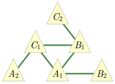This problem can be reduced to identifying the injectable pairs of nodes, because if all of the pairs in a set of nodes are <details> <summary>Image 9 Details</summary>  ### Visual Description ## Hierarchical Diagram: Node Relationships ### Overview The image depicts a hierarchical network of six triangular nodes labeled A1, A2, B1, B2, C1, and C2. Green lines connect nodes in a structured, tiered arrangement, suggesting dependencies or relationships between components. The diagram lacks a legend, axis titles, or numerical data, focusing purely on structural relationships. ### Components/Axes - **Nodes**: - Bottom tier: A1 (central), A2 (left) - Middle tier: B1 (right), C1 (left) - Top tier: C2 (center) - **Connections**: - A1 ↔ A2 (horizontal) - A1 ↔ B1 (diagonal) - A1 ↔ C1 (diagonal) - B1 ↔ B2 (horizontal) - B1 ↔ C1 (diagonal) - C1 ↔ C2 (vertical) - **Legend**: Absent. Line color (green) is uniform but lacks explicit meaning. ### Detailed Analysis - **Node Placement**: - A1 is centrally located at the base, acting as a root node with three outgoing connections. - A2 branches left from A1, forming a secondary path. - B1 and C1 occupy the middle tier, with B1 connecting to B2 (right) and C1 connecting upward to C2. - C2 sits at the apex, directly linked to C1. - **Flow Direction**: - Primary flow is upward (A → B → C), with lateral connections (A1 ↔ A2, B1 ↔ B2). - No feedback loops or bidirectional arrows are present. ### Key Observations 1. **Centrality of A1**: A1 serves as the primary hub, connecting to all other nodes except B2 and C2. 2. **Symmetry**: The diagram exhibits partial symmetry, with A1 and B1 both having two outgoing connections. 3. **Missing Labels**: No explicit labels for edges or nodes beyond alphanumeric identifiers (e.g., "A1" instead of descriptive terms). 4. **Color Uniformity**: All connections use green lines, but no legend clarifies their significance (e.g., strength, type of relationship). ### Interpretation This diagram likely represents a **decision tree**, **organizational hierarchy**, or **data flow architecture**. The absence of a legend limits interpretation of line colors, but the tiered structure implies: - **Dependency Chains**: Lower-tier nodes (A1, A2) feed into middle-tier nodes (B1, C1), which in turn influence the top-tier node (C2). - **Redundancy**: A1’s multiple connections suggest it may represent a critical decision point with branching outcomes. - **Isolation of C2**: C2 has no outgoing connections, indicating it may represent a final state or endpoint. The lack of numerical data or explicit labels makes quantitative analysis impossible. However, the hierarchical design emphasizes **modularity** and **sequential processing**, common in systems where inputs (A-tier) are transformed through intermediate stages (B/C-tier) to produce outputs (C2). </details> FIG. 9. The injection graph corresponding to the Spiral inflation of the Triangle scenario (Fig. 3), wherein the cliques are the injectable sets. FIG. 10. The ai-expressibility graph corresponding to the Spiral inflation of the Triangle scenario (Fig. 3), wherein two injectable sets are adjacent iff they are ancestrally independent. A set of nodes is ai-expressible iff it arises as a union of sets that form a clique in this graph. 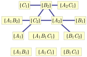<details> <summary>Image 10 Details</summary>  ### Visual Description ## Hierarchical Network Diagram: Node Relationships ### Overview The image depicts a hierarchical network diagram with interconnected nodes labeled using set notation (e.g., {C1}, {A1B1C1}). Nodes are connected via blue lines, forming a tree-like structure with multiple levels of aggregation. The diagram emphasizes relationships between discrete components through combinatorial labeling. ### Components/Axes - **Nodes**: 13 distinct nodes labeled with set notation: - Top tier: {C1}, {B2}, {A2C1} - Middle tier: {A1B2}, {C2}, {A2}, {B1} - Bottom tier: {A1}, {A1B1C1}, {B1C2} - Base tier: {A1B1}, {A1C1}, {B1C1} - **Connections**: Blue lines represent relationships between nodes. No legend is present, and all connections use the same color. - **Spatial Layout**: - Top tier nodes positioned at the apex - Middle tier nodes form a triangular connection pattern - Bottom tier nodes branch downward - Base tier nodes appear at the lowest level ### Detailed Analysis 1. **Node Labeling Patterns**: - Single-element sets: {A1}, {B1}, {C1} - Two-element combinations: {A1B1}, {A1C1}, {B1C1} - Three-element combinations: {A1B1C1} - Hybrid labels: {A2C1}, {A1B2} (mixed case notation) 2. **Connection Logic**: - Top-tier {C1} connects to {B2} and {A2C1} - Middle-tier {A1B2} connects to {C2} and {A2} - {C2} connects to {A1} and {A1B1C1} - {A2} connects to {B1} and {B1C2} - Base-tier nodes ({A1B1}, {A1C1}, {B1C1}) have no outgoing connections 3. **Structural Hierarchy**: - Three distinct levels of aggregation: - Level 1: Single elements - Level 2: Pair combinations - Level 3: Triple combinations - Top-down flow from {C1}/{B2}/{A2C1} to base-tier nodes ### Key Observations - **Combinatorial Complexity**: Each level increases in combinatorial complexity (1→2→3 elements) - **Asymmetrical Branching**: Middle-tier nodes have varying numbers of connections (2-3) - **Label Consistency**: All labels use curly brace notation with uppercase letters and numbers - **Missing Elements**: No explicit root node or terminal nodes beyond base tier ### Interpretation This diagram likely represents: 1. **Data Structure**: A tree-based data model where nodes represent sets and connections indicate parent-child relationships 2. **Dependency Graph**: Illustrating how higher-level components (e.g., {A1B1C1}) depend on lower-level elements ({A1}, {B1}, {C1}) 3. **Combinatorial System**: Visualizing all possible combinations of three elements (A, B, C) with varying inclusion levels The absence of numerical values suggests this is a conceptual model rather than a quantitative analysis. The uniform blue connections imply equal weighting between relationships, while the hierarchical layout emphasizes top-down information flow. The mixed-case labels ({A2C1} vs {A1B2}) might indicate different categorization rules for hybrid nodes versus pure combinations. </details> FIG. 11. The simplicial complex of ai-expressible sets for the Spiral inflation of the Triangle scenario (Fig. 3). The 5 facets correspond to the maximal ai-expressible sets, namely { A 1 B 1 C 1 } , { A 1 B 2 C 2 } , { A 2 B 1 C 2 } , { A 2 B 2 C 1 } and { A 2 B 2 C 2 } . 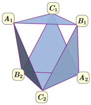<details> <summary>Image 11 Details</summary>  ### Visual Description ## 3D Geometric Diagram: Polyhedron Structure with Labeled Vertices ### Overview The image depicts a 3D geometric structure resembling a polyhedron with labeled vertices (A₁, A₂, B₁, B₂, C₁, C₂). The diagram uses color-coded regions (light blue, dark blue, purple) to differentiate spatial relationships. The structure includes triangular and quadrilateral faces, with edges connecting the vertices. ### Components/Axes - **Vertices**: - **A₁**: Top-left vertex (light blue region). - **A₂**: Bottom-right vertex (dark blue region). - **B₁**: Top-right vertex (light blue region). - **B₂**: Bottom-left vertex (dark blue region). - **C₁**: Top-center vertex (purple region). - **C₂**: Bottom-center vertex (purple region). - **Edges**: - Connect A₁-B₁, B₁-C₁, C₁-A₁ (top triangular face). - Connect A₂-B₂, B₂-C₂, C₂-A₂ (bottom triangular face). - Diagonal edges: A₁-B₂, B₁-C₂, A₂-C₁ (interconnecting regions). - **Legend**: - **Light Blue**: Top-left and top-right regions (A₁, B₁). - **Dark Blue**: Bottom-left and bottom-right regions (A₂, B₂). - **Purple**: Central regions (C₁, C₂). - **Spatial Grounding**: - Legend positioned at the bottom-right corner. - Vertices labeled with black text on white backgrounds. ### Detailed Analysis - **Color-Coded Regions**: - Light blue regions dominate the upper portion (A₁, B₁). - Dark blue regions occupy the lower portion (A₂, B₂). - Purple regions (C₁, C₂) act as transitional zones between upper and lower sections. - **Edge Relationships**: - Diagonal edges (e.g., A₁-B₂) create intersecting planes, suggesting a non-convex polyhedron. - Triangular faces (top and bottom) are highlighted with solid lines, while quadrilateral faces use dashed lines. ### Key Observations 1. **Symmetry**: The structure exhibits bilateral symmetry along the vertical axis (C₁-C₂). 2. **Color Coding**: Purple regions (C₁, C₂) serve as bridges between light blue and dark blue zones. 3. **Non-Convexity**: The intersecting diagonal edges imply a concave or complex polyhedral shape. ### Interpretation This diagram likely represents a geometric model for spatial analysis, such as a Voronoi diagram, Delaunay triangulation, or a 3D mesh for computational geometry. The color coding may indicate zones of influence, material properties, or connectivity constraints. The absence of numerical data suggests the focus is on structural relationships rather than quantitative metrics. The intersecting edges and transitional purple regions highlight potential areas of overlap or interaction between distinct zones. </details> injectable, then so too is the set itself. This can be proven as follows. Let ϕ : G ′ → G be the projection map from G ′ to the original causal structure G , corresponding to removing copy-indices. Then ϕ has the characteristic feature that it preserves and reflects edges: if A → B in G ′ , then also ϕ ( A ) → ϕ ( B ) in G , and vice versa; this follows from the assumption that G ′ is an inflation of G . A set V ⊆ ObservedNodes ( G ′ ) is injectable if and only if the restriction of ϕ to An ( V ) is an injective map. But now injectivity of a map means precisely that no two different elements of the domain get mapped to the same element of the codomain. So if V is injectable, then so is each of its two-element subsets; conversely, if V is not injectable, then ϕ maps two nodes among the ancestors of V to the same node, which means that there are two nodes in the ancestry that differ only by copy-index. Each of these two nodes must be an ancestor of at least some node in V ; if one chooses two such descendants, then one gets a two-element subset of V such that ϕ is not injective on the ancestry of that subset, and therefore this two-element set of observed nodes is not injectable. To enumerate the injectable sets, it is therefore useful to encode certain features of the inflated causal structure in an undirected graph which we call the injection graph . The nodes of the injection graph are the observed nodes of the inflated causal structure, and a pair of nodes A i and B j share an edge if the pair { A i B j } is injectable. For example, Fig. 9 shows the injection graph of the Spiral inflation of the Triangle scenario (Fig. 3). The property noted above states that the injectable sets are precisely the cliques 18 of the injection graph. While for many other applications only the maximal cliques are of interest, our application of the inflation technique requires knowledge of all nonempty cliques. Given a list of the injectable sets, the ai-expressible sets can be read off from the ai-expressability graph . The nodes of the ai-expressibility graph are taken to be the injectable sets in G ′ , and two nodes share an edge if the associated injectable sets are ancestrally independent. Fig. 10 depicts an example. The ai-expressible sets correspond to the cliques of the ai-expressibility graph: the union of all the injectable sets that make up the nodes of a clique is an ai-expressible set, while the individual nodes already give us the partition into injectable sets relevant for the factorization relation of Eq. (45). For our purposes, it is sufficient to enumerate the maximal ai-expressible sets, so that one only needs to consider the maximal cliques of the ai-expressibility graph. From Figs. 9 and 10, we easily infer the injectable sets and the maximal ai-expressible sets, as well as the partition of the maximal ai-expressible sets into ancestrally independent subsets. For the Spiral example, this results in: $$\begin{array} { r l } & { \underbrace { \{ A _ { 1 } \} , \, \{ B _ { 1 } \} , \, \{ C _ { 1 } \} , } _ { \substack { \{ A _ { 2 } \} , \, \{ B _ { 2 } \} , \, \{ C _ { 2 } \} , } } \underbrace { \{ A _ { 1 } B _ { 1 } C _ { 1 } \} } _ { \substack { \{ A _ { 1 } B _ { 2 } C _ { 2 } \} \\ \{ A _ { 1 } B _ { 1 } \} , \, \{ A _ { 1 } C _ { 1 } \} , \, \{ B _ { 1 } C _ { 2 } A _ { 2 } \} } } \underbrace { \{ A _ { 1 } B _ { 2 } \} \perp _ { d } \{ C _ { 2 } \} } _ { \substack { \{ B _ { 1 } C _ { 2 } \} \\ \{ C _ { 1 } A _ { 2 } B _ { 2 } \} \\ \{ A _ { 1 } B _ { 2 } \} , \, \{ A _ { 2 } C _ { 1 } \} , \, \{ B _ { 1 } C _ { 2 } A _ { 2 } \} } } \underbrace { \{ C _ { 1 } A _ { 2 } \} \perp _ { d } \{ B _ { 2 } \} } _ { \substack { \{ A _ { 2 } \} \perp _ { d } \{ B _ { 2 } \} \\ \{ A _ { 1 } B _ { 2 } C _ { 2 } \} } } \underbrace { \{ A _ { 2 } \} \perp _ { d } \{ B _ { 2 } \} \perp _ { d } \{ C _ { 2 } \} } _ { \substack { \{ A _ { 1 } B _ { 2 } \} \\ \{ A _ { 1 } B _ { 1 } C _ { 1 } \} , \, \{ A _ { 1 } B _ { 1 } C _ { 2 } \} } } } \end{array}$$ Having identified the ai-expressible sets and how they partition into injectable sets, we now infer the factorization relations implied by ancestral independences, which is Eq. (41) in the Spiral example. Next, we discuss the other ingredient of our systematic procedure: the marginal problem. 18 A clique is a set of nodes in an undirected graph any two of which share an edge. ## B. The Marginal Problem and its Solution The third step in our procedure is determining whether the given distributions on ai-expressible sets can arise as marginals of one joint distribution on all observed nodes of the inflated causal structure. In general, the problem of determining whether a given family of distributions can arise as marginals of some joint distribution is known as the marginal problem 19 . In order to derive causal compatibility inequalities, one must solve the closely related problem of determining necessary and sufficient constraints that a family of marginal distributions must satisfy in order for the marginal problem to have a solution. For better clarity, we distinguish these two variants of the marginal problem as the marginal satisfiability problem and the marginal constraint problem . The generic marginal problem will be used as an umbrella term referring to both types. To specify either sort of marginal problem, one must specify the full set of variables to be considered, denoted V , together with a family of subsets of S , denoted ( V 1 , . . . , V n ) and called contexts . The family of contexts can be visualized through the simplicial complex that it generates, as illustrated in Fig. 11. A marginal scenario consists of a specification of contexts together with a specification of the cardinality of each variable. Every joint distribution P V defines a family of marginal distributions ( P V 1 , . . . , P V n ) through marginalization, P V i := ∑ V \ V i P V . The marginal problem concerns the converse inference. In the marginal satisfiability problem, a concrete family of distributions ( P V 1 , . . . , P V n ) is given, and one wants to decide whether there exists a joint distribution ˆ P V such that P V i = ∑ V \ V i ˆ P V for all i . In the marginal constraint problem, one seeks to find conditions on the family of distributions ( P V 1 , . . . , P V n ), considered as parameters, for when a joint distribution ˆ P V exists which reproduces these as marginals, P V i = ∑ V \ V i ˆ P V for all i . In order for ˆ P V to exist, distributions on different contexts must be consistent on the intersection of contexts, that is, marginalizing P V i to those variables in the intersection V i ∩ V j must result in the same distribution as marginalizing P V j to that intersection. In many cases, this is not sufficient 20 ; indeed, we have already seen examples of additional constraints, namely, the inequalities (31), (36) and (40) from Sec. III C. So what are the necessary and sufficient conditions? To answer this question, it helps to realize two things: - The set of all valid (positive, normalized) distributions P V is precisely the convex hull of the deterministic assignments of values to V (the deterministic distributions), and - The map P V ↦→ ( P V 1 , . . . , P V n ), describing marginalization to each of the contexts in ( V 1 , . . . , V n ), is linear. Hence the image of the set of possibilities for the distribution P V under the map P V ↦→ ( P V 1 , . . . , P V n ) is exactly the convex hull of the deterministic assignments of values to ( V 1 , . . . , V n ) which are consistent where these contexts overlap. Since there are only finitely many such deterministic assignments, this convex hull is a polytope; it is called the marginal polytope [68]. Together with the above equations on coinciding submarginals, the facet inequalities of this polytope solve the marginal constraint problem. The marginal satisfiability problem asks about membership in the polytope; by the above, this becomes a linear program with the joint probabilities P V as the unknowns. To express this more concretely, we write the marginal satisfiability problem in the form of a generic linear program. Let the joint distribution vector v be the vector associated with the joint probability distribution P V , that is, the vector whose components are the probabilities P V ( v ). Let the marginal distribution vector b be the vector that is the concatenation over i of the vectors associated with the distributions P V i . Finally, let the marginal description matrix M be the matrix representation of the linear map corresponding to marginalization on each of the contexts, that is, P V → ( P V 1 , . . . , P V n ) where P V i = ∑ V \ V i P V . The components of M all take the value zero or one. In this notation, the marginal satisfiability problem consists of determining whether, for a given vector b , the following constraints are feasible: $$\exists v \, { \colon } v \geq 0 , \, M v = b ,$$ where the component-wise inequality v ≥ 0 enforces the constraint that P V is a nonnegative probability distribution. This is clearly a linear program. In the example of Fig. 11 with binary variables, M is a 48 × 64 matrix, so that Mv = b represents 48 equations and v ≥ 0 represents 64 inequalities; explicit representations of M , v , and b for the simpler example of the Cut inflation can be found in Appendix B. A single linear program can then assess whether there is a solution in v for a given marginal distribution vector b . If this is not the case, then the marginal satisfiability problem has a negative answer. 19 For further references and an outline of the long history of the marginal problem, see [35]. An alternative account using the language of presheaves can also be found in [65]. 20 Depending on how the contexts intersect with one another, this may be sufficient. A precise characterization for when this occurs has been found by Vorob'ev [66]. See also Budroni et al. [67, Thm. 2] for an application of this characterization enabling computationally significant shortcuts in solving the marginal constraint problem. Since linear programming is quite easy, probing specific distributions for compatibility for a given inflated causal structure is computationally inexpensive. For instance, using the Web inflation of the Triangle scenario (Fig. 2), which contains a large number of observed variables, our numerical computations have reproduced the result of [21, Theorem 2.16], that a certain distribution considered therein is incompatible with the Triangle scenario 21 . In the case of the marginal constraint problem, the vector b is not given, but one rather wants to find conditions on b that hold if and only if Eq. (50) has a solution. As per the above, this is a problem of facet enumeration 22 for the marginal polytope. Equivalently, it is the problem of linear quantifier elimination 23 for the system of Eq. (50): one tries to find a system of linear equations and inequalities in b such that some b satisfies the system if and only if Eq. (50) has a solution. There is a unique minimal system achieving this, and it consists of the constraints of consistency on the intersections of contexts (mentioned above), together with the facet inequalities of the marginal polytope. Taken together, these form a system of linear equations and inequalities that is equivalent to Eq. (50), but does not contain any quantifiers. In our application, the equations expressing consistency on the intersections of contexts are guaranteed to hold automatically, so that only the facet inequalities are of interest to us. In terms of Eq. (50), a valid inequality for the marginal distribution vector b -such as a facet inequality of the marginal polytope-can always be expressed as y T b ≥ 0 for some vector y . Validity of an inequality y T b ≥ 0 means precisely that y T M ≥ 0 , since the columns of M are the vertices of the marginal polytope. The marginal satisfiability problem for a given vector b 0 has no solution if and only if there is a vector y that yields a valid inequality but for which y T b 0 < 0. Necessity follows by noting that if Eq. (50) does have a solution v for a given vector b 0 , then the fact that y T M ≥ 0 and the fact that v ≥ 0 implies that y T b 0 = y T Mv ≥ 0. Sufficiency follows from Farkas' lemma. Most linear programming tools are capable of returning a Farkas infeasibility certificate [69] whenever a linear program has no solution. In our case, if the marginal problem is infeasible for a vector b 0 , then the certificate is a vector y that yields a valid inequality but for which y T b 0 < 0. 24 . Upon substituting the factorization relations of Eq. (45) and deleting copy indices, any valid inequality for the marginal problem turns into a causal compatibility inequality. This applies both to facet inequalities of the marginal polytope, and to Farkas infeasibility certificates. In the latter case, one obtains an explicit causal compatibility inequality which witnesses the given distribution as incompatible with the given causal structure. In other words, if a given distribution is witnessed as incompatible with a causal structure using the technique we have described, then with little additional numerical effort, one can also obtain a causal compatibility inequality that exhibits the incompatibility. This may have applications to problems where the facet enumeration is computationally intractable. Summarizing, we have shown how to leverage the marginal satisfiability problem to witness causal incompatibility of particular distributions, and how to leverage the marginal constraint problem to derive causal compatibility inequalities. ## C. A List of Causal Compatibility Inequalities for the Triangle scenario As an example of the above method, we have considered the Triangle scenario with binary observed variables and derived all causal compatibility inequalities which follow by means of using ancestral independences in the Spiral inflation (Fig. 3). We found that there are 4884 inequalities corresponding to the facets of the relevant marginal polytope, which results in 4884 polynomial causal compatibility inequalities for the Triangle scenario. However, most inequalities in this set have turned out to be redundant, where an inequality is considered redundant if there is no distribution that violates this inequality but none of the others. We thus have looked for a subset of inequalities that is irredundant (does not contain any redundant inequality) but nevertheless complete (defines the same set of distributions as the full set). While a finite system of linear inequalities always has a unique irredundant complete subset, this need not be the case for finite systems of polynomial inequalities; we therefore speak of 'a' complete irredundant set instead of 'the' complete irredundant set. We exploited linear programming techniques to quickly identify a 1433-inequalities complete subset of our original 4884 inequalities; concretely, the copy isomorphisms of Appendix C yield an additional list of linear equations satisfied by all inflation models, and from every set of inequalities that differ by merely a linear combination of these equations we choose one representative. To further prune away redundant inequalities, we successively employed nonlinear constrained maximization on each inequality's left-hand-side, to determine numerically if it could be violated pursuant to all the other inequalities as constraints. An inequality is found to be redundant if the solution to the constrained maximization does not exceed the inequality's right-hand side. Such an inequality was immediately dropped from 21 This distribution is , however, quantum-compatible with the Triangle scenario (Sec. V D). 22 In Appendix A, we provide an overview of techniques for facet enumeration. 23 Linear quantifier elimination has already been used in causal inference for deriving entropic causal compatibility inequalities [25, 33]. In that task, however, the unknowns being eliminated are entropies on sets of variables of which one or more is latent. By contrast, the unknowns being eliminated above are all probabilities on sets of variables all of which are observed-but on the inflated causal structure rather than the original causal structure. 24 Farkas infeasibility certificates are available in Mosek , Gurobi , and CPLEX , as well as by accessing dual variables in cvxr / cvxopt . the set before testing the next candidate for redundancy 25 . This post-processing led us to identify 60 irredundant inequalities which defines the same set of satisfying distributions as the original 4884. Of the remaining 60, we recognized 8 as uninteresting positivity inequalities, P ABC ( abc ) ≥ 0, so that our irredundant complete system consists of 52 polynomial inequalities. To present those inequalities in an efficient manner, we further grouped them into four symmetry classes. In Eqs. (51-54) we present one representative from each class; the multiplicity of inequalities contained in each symmetry class is marked in parentheses. The symmetry group for any causal structure with finite-cardinality observed variables is generated by those permutations of the observed variables which can be extended to automorphisms of the (original) DAG, as well as any permutation among the discrete values assigned to an individual observed variable (i.e., bijections on the sample space of that variable). In the case of the Triangle scenario with binary observed variables, the symmetry group therefore has 48 elements, comprised of the 6 permutations of the three observed variables, the three local binary-value relabellings, and all their compositions (48 = 6 × 2 × 2 × 2). We choose to express our inequalities in terms of correlators (where the two possible values of each variables to be {-1 , +1 } ), rather than in terms of joint probabilities, because such a presentation is more compact: $$0 \leq 1 - { \mathbb { E } } [ A C ] - { \mathbb { E } } [ B C ] + { \mathbb { E } } [ A ] { \mathbb { E } } [ B ] \quad ( \times 1 2 ) \quad ( 5 1 )$$ $$0 \leq 3 & - \mathbb { E } [ A ] - \mathbb { E } [ B ] - \mathbb { E } [ C ] + 2 \mathbb { E } [ A B ] + 2 \mathbb { E } [ A C ] + 2 \mathbb { E } [ B C ] \\ & + \mathbb { E } [ A B C ] + \mathbb { E } [ A ] \mathbb { E } [ B ] + \mathbb { E } [ A ] \mathbb { E } [ C ] + \mathbb { E } [ B ] \mathbb { E } [ C ] & ( \times 8 ) & ( 5 2 ) \\ & - \mathbb { E } [ A ] \mathbb { E } [ B C ] - \mathbb { E } [ B ] \mathbb { E } [ A C ] - \mathbb { E } [ C ] \mathbb { E } [ A B ] + \mathbb { E } [ A ] \mathbb { E } [ B ] \mathbb { E } [ C ]$$ $$0 \leq 4 + & 2 \mathbb { E } [ C ] - 2 \mathbb { E } [ A B ] - 3 \mathbb { E } [ A C ] - 2 \mathbb { E } [ B C ] - \mathbb { E } [ A B C ] + \mathbb { E } [ A ] \mathbb { E } [ B ] \mathbb { E } [ C ] & ( \times 2 4 ) & ( 5 3 ) \\ & + 2 \mathbb { E } [ A ] \mathbb { E } [ B ] + \mathbb { E } [ A ] \mathbb { E } [ C ] - \mathbb { E } [ A ] \mathbb { E } [ B C ] - \mathbb { E } [ C ] \mathbb { E } [ A B ]$$ $$0 \leq 4 - 2 & { \mathbb { E } } [ A B ] - 2 { \mathbb { E } } [ A C ] - 2 { \mathbb { E } } [ B C ] - { \mathbb { E } } [ A B C ] \\ & + 2 { \mathbb { E } } [ A ] { \mathbb { E } } [ B ] + 2 { \mathbb { E } } [ A ] { \mathbb { E } } [ C ] + 2 { \mathbb { E } } [ B ] { \mathbb { E } } [ C ] & ( \times 8 ) & ( 5 4 ) \\ & - { \mathbb { E } } [ A ] { \mathbb { E } } [ B C ] - { \mathbb { E } } [ B ] { \mathbb { E } } [ A C ] - { \mathbb { E } } [ C ] { \mathbb { E } } [ A B ]$$ All the inequalities (51-54) have no slack in the sense that they can be saturated by distributions compatible with the Triangle scenario. Indeed, all the inequalities are saturated by the deterministic distribution E [ A ]= E [ B ]= E [ C ]=1, except for Eq. (52) which is saturated by the deterministic distribution E [ A ]= E [ B ]= -E [ C ]=1. Generally speaking, any polynomial inequality generated by a facet of the marginal polytope (i.e. corresponding to some linear inequality in the variables of the inflated causal structure) will be saturated by some deterministic distribution. A machine-readable and closed-under-symmetries version of this list of inequalities may be found in Appendix F. ## D. Causal Compatibility Inequalities via Hardy-type Inferences from Logical Tautologies Enumerating all the facets of the marginal polytope is computationally feasible only for small examples. But our method transforms every inequality that bounds the marginal polytope into a causal compatibility inequality. We now present a general approach for deriving a special type of such inequalities very quickly. In the literature on Bell inequalities, it has been noticed that incompatibility with the Bell causal structure can sometimes be witnessed by merely looking at which joint outcomes have zero probability and which ones have nonzero probability. In other words, instead of considering the probability of an outcome, the inconsistency of some marginal distributions can be evident from considering only the possibility or impossibility of each outcome. This insight is originally due to Hardy [49], and versions of Bell's theorem that are based on the violation of such possibilistic constraints are known as Hardy-type paradoxes [57, 70-73]; a partial classification of these can be found in [50]. The method that we describe in the second half of this section can be used to compute a complete classification of possibilistic constraints for any marginal problem. Possibilistic constraints follow from a consideration of logical relations that can hold among deterministic assignments to the observed variables. Such logical constraints can also be leveraged to derive probabilistic constraints instead of possibilistic ones, as shown in [60, 74]. This results in a partial solution to any given (probabilistic) marginal problem. Essentially, we solve a possibilistic marginal problem [50], then upgrade the possibilistic constraints into probabilistic 25 It is advantageous to group the inequalities into symmetry classes prior to pruning away redundant inequalities, so that entire classes of inequalities can be discarded when finding that a single representative is redundant to the other classes . inequalities, resulting in a set of probabilistic inequalities whose satisfaction is a necessary but insufficient condition for satisfying the corresponding probabilistic marginal problem. We now demonstrate how to systematically derive all inequalities of this type. We have already provided a simple example of a Hardy-type argument in Example 2, in the logic used to demonstrate that the family of distributions of Eqs. (17-19) cannot arise as the marginals of a single joint distribution. For our present purposes, it is useful to recast that argument into a new but manifestly equivalent form. First, for the family of distributions in question, we have <!-- formula-not-decoded --> From the last constraint one infers that at least one of A 1 , B 1 and C 1 must be 1, which from the three other constraints implies that at least one of A 2 , B 2 and C 2 must be 0, so that it is not the case that all of A 2 , B 2 and C 2 are 1. Thus Eq. (55) implies $$\text {Never} \quad A _ { 2 } = & 1 \text { and } B _ { 2 } = & 1 \text { and } C _ { 2 } = & 1 .$$ However, the Spiral inflation (Fig. 3) is such that A 2 , B 2 , and C 2 have no common ancestor and consequently the distribution on the ai-expressible set { A 2 B 2 C 2 } is the product of the distributions on A 2 , B 2 and C 2 . Since each of the latter has full support (Eq. (19)), it follows that the distribution on { A 2 B 2 C 2 } also has full support, which contradicts Eq. (56). We are here interested in recasting the argument in a manner amenable to systematic generalization. This is done as follows. We work in a marginal scenario where the contexts are { A 2 B 2 C 2 } , { A 2 C 1 } , { B 2 A 1 } , { C 2 B 1 } , and { A 1 B 1 C 1 } , and all variables are binary. The first step of the argument is to note that 26 $$\neg [ A _ { 2 } = & \, 1 , C _ { 1 } = 1 ] \bigwedge ^ { - [ B _ { 2 } = 1 , \, A _ { 1 } = 1 ] } \bigwedge ^ { - [ C _ { 2 } = 1 , \, B _ { 1 } = 1 ] } \bigwedge ^ { - [ A _ { 1 } = 0 , \, B _ { 1 } = 0 , \, C _ { 1 } = 0 ] } \\ & \implies \neg [ A _ { 2 } = 1 , B _ { 2 } = 1 , C _ { 2 } = 1 ] .$$ is a logical tautology for binary variables. It can be understood as a constraint on marginal deterministic assignments , which can be thought of as a logical counterpart of a linear inequality bounding the marginal polytope. The second and final step of the argument notes that the given marginal distributions are such that the antecedent is always true, while the consequent is sometimes false. To see how to translate this into a constraint on marginal distributions , we rewrite Eq. (57) in its contrapositive form, $$[ A _ { 2 } = 1 , B _ { 2 } = 1 , C _ { 2 } = 1 ] \Rightarrow [ A _ { 2 } = 1 , C _ { 1 } = 1 ] \vee [ B _ { 2 } = 1 , A _ { 1 } = 1 ] \vee [ C _ { 2 } = 1 , B _ { 1 } = 1 ] \vee [ A _ { 1 } = 0 , B _ { 1 } = 0 , C _ { 1 } = 0 ] .$$ Next, we note that if a logical tautology can be expressed as $$E _ { 0 } \implies E _ { 1 } \lor \dots \lor E _ { n } ,$$ then by applying the union bound-which asserts that the probability of at least one of a set of events occurring is no greater than the sum of the probabilities of each event occurring-one obtains $$P ( E _ { 0 } ) \leq \sum _ { j = 1 } ^ { n } P ( E _ { j } ) .$$ Applying this to Eq. (58) in particular yields $$P _ { A _ { 2 } B _ { 2 } C _ { 2 } } ( 1 1 1 ) \leq P _ { A _ { 1 } B _ { 2 } } ( 1 1 ) + P _ { B _ { 1 } C _ { 2 } } ( 1 1 ) + P _ { A _ { 2 } C _ { 1 } } ( 1 1 ) + P _ { A _ { 1 } B _ { 1 } C _ { 1 } } ( 0 0 0 ) ,$$ which is a constraint on the marginal distributions . 26 Here, ∧ , ∨ and ¬ denote conjunction, disjunction and negation respectively. This inequality allows one to demonstrate the incompatibility of the family of distributions of Eqs. (17-19) with the Spiral inflation just as easily as one can with the tautology of Eq. (57). The fact that A 2 , B 2 and C 2 are ancestrally independent in the Spiral inflation implies that P A 2 B 2 C 2 = P A 2 P B 2 P C 2 . It then suffices to note that for the given family of distributions, the probability on the left-hand side of Eq. (61) is nonzero (which corresponds to the consequent of Eq. (57) being sometimes false) while every probability on the right-hand side is zero (which corresponds to the antecedent of Eq. (57) being always true). But, of course, the inequality can witness many other incompatibilities in addition to this one. As another example, consider the marginal problem where the variables are A , B and C , with each being binary, and the contexts are the pairs { AB } , { AC } , and { BC } . The following tautology provides a constraint on marginal deterministic assignments: 27 $$[ A = 0 , C = 0 ] \implies [ A = 0 , B = 0 ] \vee [ B = 1 , C = 0 ] .$$ Applying the union bound, one obtains a constraint on marginal distributions, 28 $$P _ { A C } ( 0 0 ) \leq P _ { A B } ( 0 0 ) + P _ { B C } ( 1 0 ) .$$ In this section, we seek to determine, for any marginal scenario, the set of all inequalities that can be derived in this manner. We do so by enumerating the full set of tautologies of the form of Eqs. (57,62). This boils down to solving the possibilistic version of the marginal constraint problem. We now describe the general procedure. As before, we express a constraint on marginal deterministic assignments as a logical implication, having a valuation (assignment of outcomes) on one context as the antecedent and a disjunction over valuations on contexts as the consequent . In the following, we explain how to generate all such implications which are tight in the sense that the consequent is minimal, i.e., involves as few terms as possible in the disjunction. First, we fix the antecedent by choosing some context and a joint valuation of its variables. In order to generate all constraints on marginal deterministic assignments, one will have to perform this procedure for every context as the antecedent and every choice of valuation thereon. For the sake of concreteness, we take the above Spiral inflation example with [ A 2 = 1 , B 2 = 1 , C 2 = 1 ] as the antecedent. Each logical implication we consider is required to have the property that any variable that appears in both the antecedent and the consequent must be given the same value in both. To formally determine all valid consequents, it is useful to introduce two hypergraphs associated to the problem. Recall the definition of the incidence matrix of a hypergraph: if vertex i is contained in edge j of the hypergraph, the component in the i th row and j th column of the matrix is 1; otherwise it is 0. The first hypergraph we consider is the one whose incidence matrix is the marginal description matrix M for the marginal problem being considered, as introduced near Eq. (50). Each vertex in this hypergraph corresponds to a valuation on some particular context. Each hyperedge corresponds to a possible joint valuation of all the variables. A hyperedge contains a vertex if the valuation represented by the hyperedge is an extension of the valuation represented by the vertex. For example, the hyperedge [ A 1 =0 , A 2 = 1 , B 1 =0 , B 2 = 1 , C 1 =1 , C 2 = 1 ] contains the vertex [ A 1 =0 , B 2 = 1 , C 2 = 1 ]. In our example following Fig. 11, this initial hypergraph has 5 · 2 3 = 40 vertices and 2 6 = 64 hyperedges. The second hypergraph is a subhypergraph of the first one. We delete from the first hypergraph all vertices and hyperedges which contradict the outcomes supposed by the antecedent. In our example, because the vertex [ A 2 = 1 , B 2 = 0 , C 1 =1] contradicts the antecedent [ A 2 = 1 , B 2 = 1 , C 2 = 0 ], we delete it. We also delete the vertex corresponding to the antecedent itself. In our example, this second hypergraph has 2 3 +3 · 2 1 = 14 vertices and 2 3 = 8 hyperedges. All valid (minimal) consequents are (minimal) transversals of this latter hypergraph. A transversal is a set of vertices which has the property that it intersects every hyperedge in at least one vertex. In order to get implications which are as tight as possible, it is sufficient to enumerate only the minimal transversals. Doing so is a well-studied problem in computer science with various natural reformulations and for which manifold algorithms have been developed [75]. In our example, it is not hard to check that the consequent of $$\begin{array} { r l } { [ A _ { 2 } = 1 , B _ { 2 } = 1 , C _ { 2 } = 1 ] } & { \Longrightarrow \quad [ A _ { 1 } = 1 , B _ { 2 } = 1 , C _ { 2 } = 1 ] \vee [ A _ { 2 } = 1 , B _ { 1 } = 1 , C _ { 2 } = 1 ] } \\ & { \quad \vee [ A _ { 2 } = 1 , B _ { 2 } = 1 , C _ { 1 } = 1 ] \vee [ A _ { 1 } = 0 , B _ { 1 } = 0 , C _ { 1 } = 0 ] } \end{array}$$ 27 This is a tautology since E ∧ F = ⇒ E ∧ F ∧ ( G ∨ ¬ G ) = ( E ∧ F ∧ G ) ∨ ( E ∧ F ∧ ¬ G ) = ⇒ ( E ∧ G ) ∨ ( F ∧ ¬ G ). 28 This inequality is equivalent to Eq. (31). is such a minimal transversal: every assignment of values to all variables which extends the assignment on the left-hand side satisfies at least one of the terms on the right, but this ceases to hold as soon as one removes any one term on the right. We convert these implications into inequalities in the usual way via the union bound (i.e., replacing ' ⇒ ' by ' ≤ ' at the level of probabilities and the disjunction by summation). Thus Eq. (63) translates into the constraint on marginal distributions $$P _ { A _ { 2 } B _ { 2 } C _ { 2 } } ( 1 1 1 ) \leq P _ { A _ { 1 } B _ { 2 } C _ { 2 } } ( 1 1 1 ) + P _ { A _ { 2 } B _ { 1 } C _ { 2 } } ( 1 1 1 ) + P _ { A _ { 2 } B _ { 2 } C _ { 1 } } ( 1 1 1 ) + P _ { A _ { 1 } B _ { 1 } C _ { 1 } } ( 0 0 0 ) .$$ This inequality constitutes a strengthening of Eq. (61) that we had used as Eq. (40) as the starting point for deriving a causal compatibility inequality for the Triangle scenario, Eq. (43). Inequalities that one derives from hypergraph transversals are generally weaker than those that result from a complete solution of the marginal problem. Nevertheless, many Bell inequalities are of this form, the CHSH inequality among them [74]. So it seems that this method is still sufficiently powerful to generate plenty of interesting inequalities. At the same time, the method is significantly less computationally costly than the full-fledged facet enumeration, even if one does it for every possible antecedent. Interestingly, all of the irredundant polynomial inequalities represented in Eqs. (51-54) are found to be derivable by means of hypergraph transversals. In conclusion, facet enumeration is the preferred method for deriving inequalities for the marginal problem when it is computationally tractable. When it is not, enumerating hypergraph transversals presents a good alternative. ## V. FURTHER PROSPECTS FOR THE INFLATION TECHNIQUE Lemma 4 and Corollary 6 state that any causal inference technique on an inflated causal structure G ′ can be transferred to the original causal structure G . In the previous section, we have found that even extremely weak techniques on G ′ -namely the constraints implied by the existence of a joint distribution together with ancestral independences-can lead to significant and new results for causal inference on G . In the following three subsections, we consider some additional possibilities for constraints that might be exploited in this way to enhance the power of inflation further. ## A. Appealing to d -Separation Relations in the Inflated Causal Structure beyond Ancestral Independance In Sec. IV, we considered the inflation technique using sets of observed variables on the inflated causal structure that were ai-expressible, that is, that can be written as a union of injectable sets that are ancestrally independent. However, it is standard practice when deriving causal compatibility conditions for a causal structure to make use not just of ancestral independences, but of arbitrary d -separation relations among variables, and for this reason we had also introduced the notion of expressible set in Sec. IV. We now comment on the utility of general expressible sets for the inflation technique. In a given causal structure, if sets of variables X and Y are d -separated 29 by Z , denoted X ⊥ d Y | Z , then a distribution is compatible with that causal structure only if it satisfies the conditional independence relation X ⊥ ⊥ Y | Z , that is, ∀ xyz : P XY | Z ( xy | z ) = P X | Z ( x | z ) P Y | Z ( y | z ). In terms of unconditioned probabilities, this reads $$\forall x y z \colon P _ { X Y Z } ( x y z ) P _ { Z } ( z ) = P _ { X Z } ( x z ) P _ { Y Z } ( y z ) .$$ For Z = ∅ , d -separation of X and Y relative to Z is simply ancestral independence of X and Y , and we infer factorization of the distribution on X and Y . So it is natural to ask: can the inflation technique make use of arbitrary d -separation relations among sets of observed variables? The answer is that it can. Consider an inflation G ′ wherein X ′ and Y ′ are d -separated by Z ′ and moreover where the sets X ′ ∪ Z ′ , Y ′ ∪ Z ′ and Z ′ are injectable. In such an instance, the distribution on ∪ X ′ ∪ Y ′ ∪ Z ′ can be inferred exclusively from distributions on injectable sets, $$P _ { X ^ { \prime } Y ^ { \prime } Z ^ { \prime } } ( x y z ) = \begin{cases} \frac { P _ { X ^ { \prime } Z ^ { \prime } } ( x z ) P _ { Y ^ { \prime } Z ^ { \prime } } ( y z ) } { P _ { Z ^ { \prime } } ( z ) } & \text { if $P_{Z^{\prime}}(z)>0$} , \\ 0 & \text { if $P_{Z^{\prime}}(z)=0$} . \end{cases}$$ 29 The notion of d -separation is treated at length in [1, 3, 19, 22], so we elect not to review it here. It follows that if one includes expressible sets such as X ′ ∪ Y ′ ∪ Z ′ in the set of contexts defining the marginal problem, then this simply increases the number of given marginal distributions, and one can solve the marginal problem as before by linear programming techniques. In the case where one derives inequalities on the marginal distributions, these remain linear inequalities, but ones that now include the joint probabilities P X ′ Y ′ Z ′ ( xyz ). Upon substituting conditional independence relations such as Eq. (66) in order to derive causal compatibility inequalities, one still ends up with polynomial inequalities, as in the case of using ai-expressible sets only, after multiplying by the denominators. As before, these causal compatibility inequalities for the inflation are translated into polynomial causal compatibility inequalities for the original causal structure per Corollary 6. In Appendix D, we provide a concrete example of how a d -separation relation distinct from ancestral independence can be useful both for the problem of witnessing the incompatibility of a specific distribution with a causal structure and for the problem of deriving causal compatibility inequalities. Per Definition 7, the notion of expressibility is recursive: The set X ′ ∪ Y ′ ∪ Z ′ is expressible if X ′ ⊥ d Y ′ | Z ′ and X ′ ∪ Z ′ , Y ′ ∪ Z ′ and Z ′ are all expressible. In general, one can obtain stronger causal compatibility inequalities, and stronger witnessing power when testing the compatibility of a specific distribution, by determining the maximal expressible sets instead of restricting attention to the maximal ai-expressible sets. ## B. Imposing Symmetries from Copy-Index-Equivalent Subgraphs of the Inflated Causal Structure By the definition of an inflation model (Definition 3), if two variables in the inflated causal structure G ′ are copy-index-equivalent, A i ∼ A j , then each depends on its parents in the same fashion as A depends on its parents in the original causal structure G , meaning that P A i | Pa G ′ ( A i ) = P A | Pa G ( A ) and P A j | Pa G ′ ( A j ) = P A | Pa G ( A ) . Thus by transitivity, also A i and A j have the same dependence on their parents, $$P _ { A _ { i } | P a _ { G ^ { \prime } } ( A _ { i } ) } = P _ { A _ { j } | P a _ { G ^ { \prime } } ( A _ { j } ) } .$$ The ancestral subgraphs of A i and A j are also equivalent, and consequently equations like Eq. (67) also hold for all of the ancestors of A i and A j . We conclude that the marginal distributions of A i and A j must also be equal, P A i = P A j . More generally, it may be possible to find pairs of contexts in G ′ of any size such that constraints of the form of Eq. (67) imply that the marginal distributions on these two contexts must be equal. For example, consider the pair of contexts { A 1 A 2 B 1 } and { A 1 A 2 B 2 } for the marginal scenario defined by the Spiral inflation (Fig. 3). Neither of these two contexts is an injectable set. Nonetheless, because of Eq. (67), we can conclude that their marginal distributions coincide in any inflation model, $$\forall a a ^ { \prime } b \, \colon \, P _ { A _ { 1 } A _ { 2 } B _ { 1 } } ( a a ^ { \prime } b ) = P _ { A _ { 1 } A _ { 2 } B _ { 2 } } ( a a ^ { \prime } b ) .$$ We can similarly conclude that in the inflation model these marginal distributions satisfy P A 1 A 2 B 1 = P A 2 A 1 B 2 -where now the order of A 1 and A 2 is opposite on the two sides of the equation-or equivalently, $$\forall a a ^ { \prime } b \, \colon \, P _ { A _ { 1 } , A _ { 2 } B _ { 1 } } ( a a ^ { \prime } b ) = P _ { A _ { 1 } A _ { 2 } B _ { 2 } } ( a ^ { \prime } a b ) .$$ These constraints entail that P A 1 A 2 B 2 must be symmetric under exchange of A 1 and A 2 , which in itself is another equation of the type above. Parameters such as P A 1 A 2 B 1 ( a 1 a 2 b ), P A 1 A 2 B 2 ( a 1 a 2 b ) and P A 1 A 2 ( a 1 a 2 ) can each be expressed as sums of the unknowns P A 1 A 2 B 1 B 2 C 1 C 2 ( a 1 a 2 b 1 b 2 c 1 c 2 ), so that each equation like Eqs. (68,69) can be added to the system of equations and inequalities that constitute the starting point of the satisfiability problem (if one is seeking to test the compatibility of a given distribution with the inflated causal structure) or the quantifier elimination problem (if one is seeking to derive causal compatibility inequalities for the inflated causal structure). If any such additional relation yields stronger constraints at the level of the inflated causal structure, then one may obtain stronger constraints at the level of the original causal structure. The general problem of finding pairs of contexts in the inflated causal structure for which relations of copy-indexequivalence imply equality of the marginal distributions, and the conditions under which such equalities may yield tighter inequalities, are discussed in more detail in Appendix C. ## C. Incorporating Nonlinear Constraints In deriving causal compatibility inequalities and in witnessing causal incompatibility of a specific distribution, we restricted ourselves to starting from the marginal problem where the contexts are the (ai-)expressible sets, and wherein one imposes only linear constraints derived from the marginal problem. In this approach, facts about the causal structure only get incorporated in the construction of the marginal distribution on each expressible set, and the quantifier elimination step of the computational algorithm is linear. However, one can also incorporate facts about the causal structure as constraints on the quantifier elimination problem at the cost making the quantifier elimination problem nonlinear. Take the Spiral inflation of the Triangle scenario as an example. There is an ancestral independence therein that we did not use in our previous application of the inflation technique, namely, A 1 A 2 ⊥ d C 2 . It was not used because { A 1 A 2 C 2 } is not an expressible set. Nonetheless, we can incorporate this ancestral independence as an additional constraint in the quantifier elimination problem, namely, $$\forall a _ { 1 } a _ { 2 } c _ { 2 } \colon P _ { A _ { 1 } A _ { 2 } C _ { 2 } } ( a _ { 1 } a _ { 2 } c _ { 2 } ) = P _ { A _ { 1 } A _ { 2 } } ( a _ { 1 } a _ { 2 } ) P _ { C _ { 2 } } ( c _ { 2 } ) .$$ Recall that in the marginal problem, one seeks to eliminate the unknowns P A 1 A 2 B 1 B 2 C 1 C 2 ( a 1 a 2 b 1 b 2 c 1 c 2 ) from a set of linear equalities that define the marginal distributions, such as for instance $$P _ { A _ { 2 } B _ { 2 } } ( a _ { 2 } b _ { 2 } ) = \sum _ { a _ { 1 } b _ { 1 } c _ { 1 } c _ { 2 } } P _ { A _ { 1 } A _ { 2 } B _ { 1 } B _ { 2 } C _ { 1 } C _ { 2 } } ( a _ { 1 } a _ { 2 } b _ { 1 } b _ { 2 } c _ { 1 } c _ { 2 } ) ,$$ together with linear inequalities expressing the nonnegativity of the P A 1 A 2 B 1 B 2 C 1 C 2 ( a 1 a 2 b 1 b 2 c 1 c 2 ). We can incorporate the ancestral independence A 1 A 2 ⊥ d C 2 as an additional constraint by defining a variant of the marginal problem wherein the set of linear equations such as Eq. (71) is supplemented by the nonlinear Eq. (70) when one replaces every term therein with the corresponding sum over the P A 1 A 2 B 1 B 2 C 1 C 2 ( a 1 a 2 b 1 b 2 c 1 c 2 ). We can then proceed with quantifier elimination as we did before, eliminating the unknowns P A 1 A 2 B 1 B 2 C 1 C 2 ( a 1 a 2 b 1 b 2 c 1 c 2 ) from the system of equations in order to obtain constraints that involve only joint probabilities on expressible sets. One can incorporate any d -separation relation in the inflated causal structure in this manner. For instance, if X ⊥ d Y | Z , then this implies the conditional independence relation of Eq. (65), which can be incorporated as an additional nonlinear equality constraint when eliminating the unknowns P A 1 A 2 B 1 B 2 C 1 C 2 ( a 1 a 2 b 1 b 2 c 1 c 2 ). For instance, in the Spiral inflation of the Triangle scenario (Fig. 3), the d -separation relation A 1 ⊥ d C 2 | A 2 B 2 implies the conditional independence relation $$\forall a _ { 1 } a _ { 2 } b _ { 2 } c _ { 2 } \colon P _ { A _ { 1 } A _ { 2 } B _ { 2 } C _ { 2 } } ( a _ { 1 } a _ { 2 } b _ { 2 } c _ { 2 } ) P _ { A _ { 2 } B _ { 2 } } ( a _ { 2 } b _ { 2 } ) = P _ { A _ { 1 } A _ { 2 } B _ { 2 } } ( a _ { 1 } a _ { 2 } b _ { 2 } ) P _ { A _ { 2 } B _ { 2 } C _ { 2 } } ( a _ { 2 } b _ { 2 } c _ { 2 } ) .$$ However, because { A 1 A 2 B 2 C 2 } is not an expressible set, the method of Sec. IV does not take this d -separation relation into account. However, it can be incorporated if Eq. (72) is included as an additional nonlinear constraint in the quantifier elimination problem. On the one hand, many modern computer algebra systems do have functions capable of tackling nonlinear quantifier elimination symbolically 30 . Currently, however, it is generally not practical to perform nonlinear quantifier elimination on large polynomial systems with many unknowns to be eliminated. It may help to exploit results on the concrete algebraic-geometric structure of these particular systems [11]. If one is seeking merely to assess the compatibility of a given distribution with the causal structure, then one can avoid the quantifier elimination problem and simply try and solve an existence problem: after substituting the values that the given distribution prescribes for the outcomes on ai-expressible sets into the polynomial system in terms of the unknown global joint probabilities, one must only determine whether that system has a solution. Most computer algebra systems can resolve such satisfiability questions quite easily 31 . It is also possible to use a mixed strategy of linear and nonlinear quantifier elimination, such as Chaves [9] advocates. The explicit results of [9] are directly causal implications of the original causal structure, achieved by applying a mixed quantifier elimination strategy. Perhaps further causal compatibility inequalities will be derivable by applying such a mixed quantifier elimination strategy to the inflated causal structure. ## D. Implications of the Inflation Technique for Quantum Physics and Generalized Probabilistic Theories This specialized subsection is intended specifically for those readers already somewhat proficient with fundamental concepts in quantum theory. Non-physicists may wish to skip ahead to the conclusions. 30 For example Mathematica TM 's Resolve command, Redlog 's rlposqe , or Maple TM 's RepresentingQuantifierFreeFormula . 31 For example Mathematica TM 's Reduce`ExistsRealQ function. Specialized satisfiability software such as SMT-LIB's check-sat [76] are particularly apt for this purpose. TABLE I. A comparison of different approaches for deriving constraints on compatibility at the level of the inflated causal structure, which then translate into constraints on compatibility at the level of the original causal structure. | Type of constraints imposed on the joint distribution over all observed variables in the inflated graph | General problem | → Standard algorithm(s) | Difficulty | |------------------------------------------------------------------------------------------------------------------------------------------------------------------------------------------------------------------|-------------------------------------------------------------------------------------------------------------------|-----------------------------------------------------------------------|--------------| | Marginal compatibility, i.e. the joint distribution should recover all expressible (or ai-expressible) distributions as marginals (Sec. VA). | Facet enumeration of marginal polytope (Sec. IVB) → see | Appendix A | Hard | | Marginal compatibility, i.e. the joint distribution should recover all expressible (or ai-expressible) distributions as marginals (Sec. VA). | Finding possibilistic constraints by identifying hypergraph transversals (Sec. IVD) → see Eiter et | al. [75] | Very easy | | Whenever two equivalent-up-to- copy-indices sets of observed vari- ables have ancestral subgraphs which are also equivalent-up-to- copy-indices, then the marginals over said variables must coincide (Sec. VB). | Marginal problem with addi- tional equality constraints, there- fore linear quantifier elimination (Appendix C) → | Fourier-Motzkin elimination [77-81], Equality set projection [82, 83] | Hard | | The joint distribution should sat- isfy all conditional independence relations implied by d -separation conditions on the observed vari- ables (Sec. VC). | Real (nonlinear) quantifier elimination → | Cylindrical algebraic decomposition [9] | Very hard | Recent work has sought to explore quantum generalizations of the notion of a causal model, termed quantum causal models [22, 23, 39-43]. We here use the quantum generalization that is implied by the approach of [22] and closely related to the one of [23]. The causal structures are still represented by DAGs, supplemented with a distinction between observed and latent nodes. However, the latent nodes are now associated with families of quantum channels and the observed nodes are now associated with families of quantum measurements. Observed nodes are still labelled by random variables, which represent the outcome of the associated measurement. One also makes a distinction between edges in the DAG that carry classical information and edges that carry quantum information. 32 An observed node can have incoming edges of either type: those that come from other observed nodes carry classical information, while those that come from latent nodes carry quantum information. Each quantum measurement in the set that is associated to an observed node acts on the collection of quantum systems received by this node (i.e., on the tensor product of the Hilbert spaces associated to the incoming edges). The classical variables that are received by the node act collectively as a control variable, determining which measurement in the set is implemented. Finally, the random variable that is associated to the node encodes the outcome of the measurement. All of the outgoing edges of an observed node are classical and simply broadcast the outcome of the measurement to the children nodes. A latent node can also have incoming edges that carry classical variables as well as incoming edges that carry quantum systems. Each quantum channel in the set that is associated to a latent node takes the collection of quantum systems associated to the incoming edges as its quantum input and the collection of quantum systems associated to the outgoing edges as its quantum output (the input and output spaces need not have the same dimension). The classical variables that are received by the node act collectively as a control variable, determining which channel in the set is implemented. A quantum causal model is still ultimately in the service of explaining joint distributions of observed classical variables. The joint distribution of these variables is the only experimental data with which one can confront a given quantum causal model. The basic problem of causal inference for quantum causal models, therefore, concerns the compatibility of a joint distribution of observed classical variables with a given causal structure, where the model supplementing the causal structure is allowed to be quantum, in the sense defined above. If this happens, we say that the distribution is quantumly compatible with the causal structure. One motivation for studying quantum causal models is that they offer a new perspective on an old problem in the field of quantum foundations: that of establishing precisely which of the principles of classical physics must be 32 In many cases this notion of quantum causal model can also be formulated in a manner that does not require a distinction between two kinds of edges [23]. abandoned in quantum physics. It was noticed by Fritz [21] and Wood and Spekkens [19] that Bell's theorem [51] states that there are distributions on observed nodes of the Bell causal structure that are quantumly compatible but not classically compatible with it. Moreover, it was shown in [19] that these distributions cannot be explained by any causal structure while complying with the additional principle that conditional independences should not be fine-tuned, i.e., while demanding that any observed conditional independence should be accounted for by a d -separation relation in the DAG. These results suggest that quantum theory is perhaps best understood as revising our notions of the nature of unobserved entities, and of how one represents causal dependences thereon and incomplete knowledge thereof, while nonetheless preserving the spirit of causality and the principle of no fine-tuning [39, 84, 85]. Another motivation for studying quantum causal models is a practical one. Violations of Bell inequalities have been shown to constitute resources for information processing [86-88]. Hence it seems plausible that if one can find more causal structures for which there exist distributions that are quantumly compatible but not classically so, then this quantum-classical separation may also find applications to information processing. For example, it has been shown that in addition to the Bell scenario, such a quantum-classical separation also exists in the bilocality scenario [47] and the Triangle scenario [21], and it is likely that many more causal structures with this property will be found, some with potential applicability to information processing. So for both foundational and practical reasons, there is good reason to find examples of causal structures that exhibit a quantum-classical separation. However, this is by no means an easy task. The set of distributions that are quantumly compatible with a given causal structure is quite hard to separate from the set of distributions that are classically compatible [21, 22]. For example, both the classical and quantum sets respect the conditional independence relations among observed nodes that are implied by the d -separation relations of the DAG [22], and entropic inequalities are only of very limited use [21, 89]. We hope that the inflation technique will provide better tools for finding such separations. In addition to quantum generalizations of causal models, one can define generalizations for other operational theories that are neither classical nor quantum [22, 23]. Such generalizations are formalized using the framework of generalized probabilistic theories (GPTs) [90, 91], which is sufficiently general to describe any operational theory that makes statistical predictions about the outcomes of experiments and passes some basic sanity checks. Some constraints on compatibility can be proven to be theory-independent in that they apply not only to classical and quantum causal models, but to any kind of generalized probabilistic causal model [22]. For example, the classically-valid conditional independence relations that hold among observed variables in a causal structure are all also valid in the GPT framework. Another example is the entropic monogamy inequality Eq. (39), which was proven in [22] to be GPT valid as well. These kinds of constraints are of interest because they clarify what any conceivable theory of physics must satisfy on a given causal structure. The essential element in deriving such constraints is to only make reference to the observed nodes, as done in [22]. In fact, we now understand the argument of [22] to be an instance of the inflation technique. Nonetheless, we have seen that the inflation technique often yields inequalities that hold for the classical notion of compatibility, while having quantum and GPT violations, such as the Bell inequalities of Example 3 of Sec. III B and Appendix G. In fact, inflation can be used to derive inequalities with quantum violations for the Triangle scenario as well [92]. So what distinguishes applications of the inflation technique that yield inequalities for GPT compatibility from those that yield inequalities for classical compatibility? The distinction rests on a structural feature of the inflation: Definition 10. In G ′ ∈ Inflations ( G ) , an inflationary fan-out is a latent node that has two or more children that are copy-index equivalent. The Web and Spiral inflations of the Triangle scenario, depicted in Fig. 2 and Fig. 3 respectively, contain one or more inflationary fan-outs, as does the inflation of the Bell causal structure that is depicted in Fig. 8. On the other hand, the simplest inflation of the Triangle scenario that we consider in this article, the Cut inflation depicted in Fig. 5, does not contain any inflationary fan-outs. Our main observation is that if one uses an inflation without an inflationary fan-out, then the resulting inequalities derived by the inflation technique will all be GPT valid. In other words, one can only hope to detect a GPT-classical separation if one uses an inflation that has at least one inflationary fan-out. We now explain the intuition for why this is the case. In the classical causal model obtained by inflation, the copy-index-equivalent children of an inflationary fan-out causally depend on their parent node in precisely the same way as their counterparts in the original causal structure do. For example, this dependence may be such that these two children are exact copies of the inflationary fan-out node. So when one tries to write down a GPT version of our notion of inflation, one quickly runs into trouble: in quantum theory, the no-broadcasting theorem shows that such duplication is impossible in a strong sense [93], and an analogous theorem holds for GPTs [94]. This is why in the presence of an inflationary fan-out, one cannot expect our inequalities to hold in the quantum or GPT case, which is consistent with the fact that they often do have quantum and GPT violations. On the other hand, for any inflation that does not contain an inflationary fan-out, the notion of an inflation model generalizes to all GPTs; we sketch how this works for the case of quantum theory. By the definition of inflation, any node in G ′ has a set of incoming edges equivalent to its counterpart in G , while by the assumption that the inflated causal structure does not contain any inflationary fan-outs, any node in G ′ has either the equivalent set of outgoing edges as its counterpart in G , or some pruning of this set. In the former case, one associates to this node the same set of quantum channels (if it is a latent node) or measurements (if it is an observed node) that are associated to its counterpart. In the latter case, one simply applies the partial trace operation on the pruned edges (if it is a latent node) or a marginalization on the pruned edges (if it is an observed node). That these prescriptions make sense depends crucially on the assumption that G ′ is an inflation of G , so that the ancestries of any node in G ′ mirrors the ancestry of the corresponding node in G perfectly. Hence for inflations G ′ without inflationary fan-outs, we have quantum analogues of Lemma 4 and Corollary 6. The problem of quantum causal inference on G therefore translates into the corresponding problem on G ′ , and any constraint that we can derive on G ′ translates back to G . In particular, our Examples 1, 4 and 5 also hold for quantum causal inference: perfect correlation is not only classically incompatible with the Triangle scenario, it is quantumly incompatible as well, and the inequalities Eqs. (34,39) have no quantum violations. All of these assertions about inflations that do not contain any inflationary fan-outs apply not only to quantum causal models, but to GPT causal models as well, using the definition of the latter provided in [22]. In the remainder of this section, we discuss the relation between the quantum and the GPT case. Since quantum theory is a particular generalized probabilistic theory, quantum compatibility trivially implies GPT compatibility. Through the work of Tsirelson [54] and Popescu and Rohrlich [55], it is known that the converse is not true: the Bell scenario manifests a GPT-quantum separation. The identification of distributions witnessing this difference, and the derivation of quantum causal compatibility inequalities with GPT violations, has been a focus of much foundational research in recent years. Traditionally, the foundational question has always been: why does quantum theory predict correlations that are stronger than one would expect classically? But now there is a new question being asked: why does quantum theory only allow correlations that are weaker than those predicted by other GPTs? There has been some interesting progress in identifying physical principles that can pick out the precise correlations that are exhibited by quantum theory [95-103]. Further opportunities for identifying such principles would be useful. This motivates the problem of classifying causal structures into those which have a quantum-classical separation, those which have a GPT-quantum separation and those which have both. Similarly, one can try to classify causal compatibility inequalities into those which are GPT-valid, those which are GPT-violable but quantumly valid, and those which are quantum-violable but classically valid. The problem of deriving inequalities that are GPT-violable but quantumly valid is particularly interesting. Chaves et al. [40] have derived some entropic inequalities that can do so. At present, however, we do not see a way of applying the inflation technique to this problem. ## VI. CONCLUSIONS We have described the inflation technique for causal inference in the presence of latent variables. We have shown how many existing techniques for witnessing incompatibility and for deriving causal compatibility inequalities can be enhanced by the inflation technique, independently of whether these pertain to entropic quantities, correlators or probabilities. The computational difficulty of achieving this enhancement depends on the seed technique. We summarize the computational difficulty of the approaches that we have considered in Table I. A similar table could be drawn for the satisfiability problem, with relative difficulties preserved, but where none of the variants of the problem are computationally hard. Especially in Sec. IV, we have focused on one particular seed technique: the existence of a joint distribution on all observed nodes together with ancestral independences. We have shown how a complete or partial solution of the marginal problem for the ai-expressible sets of the inflated causal structure can be leveraged to obtain criteria for causal compatibility, both at the level of witnessing particular distributions as incompatible and deriving causal compatibility inequalities. These inequalities are polynomial in the joint probabilities of the observed variables. They are capable of exhibiting the incompatibility of the W-type distribution with the Triangle scenario, while entropic techniques cannot, so that our polynomial inequalities are stronger than entropic inequalities in at least some cases (see Example 2 of Sec. III B). As far as we can tell, our inequalities are not related to the nonlinear causal compatibility inequalities which have been derived specifically to constrain classical networks [28-30], nor to the nonlinear inequalities which account for interventions to a given causal structure [53, 104]. We have shown that some of the causal compatibility inequalities we derive by the inflation technique are necessary conditions not only for compatibility with a classical causal model, but also for compatibility with a causal model in any generalized probabilistic theory, which includes quantum causal models as a special case. It would be enlightening to understand the general extent to which our polynomial inequalities for a given causal structure can be violated by a distribution arising in a quantum causal model. A variety of techniques exist for estimating the amount by which a Bell inequality [105, 106] is violated in quantum theory, but even finding a quantum violation of one of our polynomial inequalities for causal structures other than the Bell scenario presents a new task for which we currently lack a systematic approach. Nevertheless, we know that there exists a difference between classical and quantum also beyond Bell scenarios [21, Theorem 2.16], and we hope that our polynomial inequalities will perform better in probing this separation than entropic inequalities do [22, 40]. We have shown that the inflation technique can also be used to derive causal compatibility inequalities that hold for arbitrary generalized probabilistic theories, a significant generalization of the results of [22]. Such inequalities are also very significant insofar as they constitute a restriction on the sorts of statistical correlations that could arise in a given causal scenario even if quantum theory is superseded by some alternative physical theory. As long as the successor theory falls within the framework of generalized probabilistic theories, the restriction will hold. Finally, an interesting question is whether it might be possible to modify our methods somehow to derive causal compatibility inequalities that hold for quantum theory and are violated by some GPT. Since the initial drafting of this manuscript, such a modification has been identified [107]. A single causal structure has an unlimited number of potential inflations. Selecting a good inflation from which strong polynomial inequalities can be derived is an interesting challenge. To this end, it would be desirable to understand how particular features of the original causal structure are exposed when different nodes in the causal structure are duplicated. By isolating which features are exposed in each inflation, we could conceivably quantify the utility for causal inference of each inflation. In so doing, we might find that inflations beyond a certain level of variable duplication need not be considered. The multiplicity beyond which further inflation is irrelevant may be related to the maximum degree of those polynomials which tightly characterize a causal scenario. Presently, however, it is not clear how to upper bound either number, though a finite upper bound on the maximum degree of the polynomials follows from the semialgebraicity of the compatible distributions, per Ref. [6]. Causal compatibility inequalities are, by definition, merely necessary conditions for compatibility. Depending on what kind of causal inference methods one uses at the level of an inflated causal structure G ′ , one may or may not obtain sufficient conditions. An interesting question is: if one only uses the existence of a joint distribution and ancestral independences at the level of G ′ , then does one obtain sufficient conditions as G ′ varies? In other words: if a given distribution is such that for every inflation G ′ , the marginal problem of Sec. IV is solvable, then is the distribution compatible with the original causal structure? This occurs for the Bell scenario, where it is enough to consider only one particular inflation (Appendix G). Significantly, since the initial drafting of this manuscript, Ref. [108] has proven that the inflation technique indeed gives necessary and sufficient conditions for causal compatibility: any incompatible distribution is witnessed as incompatible by a suitably large inflation. Ref. [108] also provides other interesting results, such as a prescription for how to generate all relevant inflations, as well as an explicit demonstration of the inflation technique as applied to Pearl's instrumental scenario. ## ACKNOWLEDGMENTS E.W. would like to thank Rafael Chaves, Miguel Navascues, and T.C. Fraser for suggestions which have improved this manuscript. T.F. would like to thank Nihat Ay and Guido Mont´ ufar for discussion and references. Part of this research was conducted while T.F. was with the Max Planck Institute for Mathematics in the Sciences. This project/publication was made possible in part through the support of grant #69609 from the John Templeton Foundation. The opinions expressed in this publication are those of the authors and do not necessarily reflect the views of the John Templeton Foundation. This research was supported in part by Perimeter Institute for Theoretical Physics. Research at Perimeter Institute is supported in part by the Government of Canada through the Department of Innovation, Science and Economic Development Canada and by the Province of Ontario through the Ministry of Economic Development, Job Creation and Trade. ## Appendix A: Algorithms for Solving the Marginal Constraint Problem By solving the marginal constraint problem, what we mean is to determine all the facets of the marginal polytope for a given marginal scenario. Since the vertices of this polytope are precisely the deterministic assignments of values to all variables, which are easy to enumerate, solving the marginal constraint problem is an instance of a facet enumeration problem : given the vertices of a convex polytope, determine its facets. This is a well-studied problem in combinatorial optimization for which a variety of algorithms are available [109]. A generic facet enumeration problem takes a matrix V ∈ R d × n , which lists the vertices as its columns, and asks for an inequality description of the set of vectors b ∈ R d that can be written as a convex combination of the vertices using weights x ∈ R n that are nonnegative and normalized, $$\left \{ b \in \mathbb { R } ^ { d } \ \Big | \ \exists x \in \mathbb { R } ^ { n } \colon \, b = V x , \ x \geq 0 , \ \sum _ { i } x _ { i } = 1 \right \} .$$ To solve the marginal problem one uses the marginal description matrix introduced in Sec. IV B as the input to the facet enumeration algorithm, i.e. V = M , see Eq. (50). The oldest-known method for facet enumeration relies on linear quantifier elimination in the form of FourierMotzkin (FM) elimination [77, 78]. This refers to the fact that one starts with the system b = V x , x ≥ 0 and ∑ i x i = 1, which is the half-space representation of a convex polytope (a simplex), and then one needs to project onto b -space by eliminating the variables x to which the existential quantifier ∃ x refers. The Fourier-Motzkin algorithm is a particular method for performing this quantifier elimination one variable at a time; when applied to Eq. (A.1), it is equivalent to the double description method [78, 110]. Linear quantifier elimination routines are available in many software tools 33 . The authors found it convenient to custom-code a linear quantifier elimination routine in Mathematica TM . Other algorithms for facet enumeration that are not based on linear quantifier elimination include the following. Lexicographic reverse search (LRS) [112] explores the entire polytope by repeatedly pivoting from one facet to an adjacent one, and is implemented in lrs . Equality Set Projection (ESP) [82, 83] is also based on pivoting from facet to facet, though its implementation is less stable 34 . These algorithms could be interesting to use in practice, since each pivoting step churns out a new facet; by contrast, Fourier-Motzkin type algorithms only generate the entire list of facets at once, after all the quantifiers have been eliminated one by one, see Ref. [113] for a recent comparative review. It may also be possible to exploit special features of marginal polytopes in order to facilitate their facet enumeration, such as their high degree of symmetry: permuting the outcomes of each variable maps the polytope to itself, which already generates a sizeable symmetry group, and oftentimes there are additional symmetries given by permuting some of the variables. This simplifies the problem of facet enumeration [114, 115], and it may be interesting to apply dedicated software 35 to the facet enumeration problem of marginal polytopes [116-118]. 33 For example MATLAB TM 's MPT2 / MPT3 , Maxima 's fourier elim , lrs 's fourier , or Maple TM 's (v17+) LinearSolve and Projection . The efficiency of most of these software tools, however, drops off markedly when the dimension of the final projection is much smaller than the initial space of the inequalities. Fast facet enumeration aided by Chernikov rules [79, 111] is implemented in cdd , PORTA , qskeleton , and skeleton . In the authors experience skeleton seemed to be the most efficient. Additionally, the package polymake offers multiple algorithms as options for computing convex hulls. 34 ESP [81-83] is supported by MPT2 but not MPT3 , and by the (undocumented) option of projection in the polytope (v0.1.2 2016-07-13) python module. 35 Such as PANDA , Polyhedral , or SymPol . The authors found SymPol to be rather effective for some small test problems, using the options ' ./sympol -a --cdd '. ## Appendix B: Explicit Marginal Description Matrix of the Cut Inflation with Binary Observed Variables The three maximal ai-expressible sets of the Cut inflation (Fig. 4 on Pg. 7) are { A 2 B 1 } , { B 1 C 1 } , and { A 2 C 1 } . Taking the variables to be binary, each ai-expressible set corresponds to 2 2 = 4 equations pertinent to the marginal problem. The three sets of equations which relate the marginal probabilities to a posited joint distribution are given by $$\forall a _ { 2 } b _ { 1 } \colon P _ { A _ { 2 } B _ { 1 } } ( a _ { 2 } b _ { 1 } ) = & \sum _ { c _ { 1 } } P _ { A _ { 2 } B _ { 1 } C _ { 1 } } ( a _ { 2 } b _ { 1 } c _ { 1 } ) , \\ \forall b _ { 1 } c _ { 1 } \colon P _ { B _ { 1 } C _ { 1 } } ( b _ { 1 } c _ { 1 } ) = & \sum _ { a _ { 2 } } P _ { A _ { 2 } B _ { 1 } C _ { 1 } } ( a _ { 2 } b _ { 1 } c _ { 1 } ) , \\ \forall a _ { 2 } c _ { 1 } \colon P _ { A _ { 2 } C _ { 1 } } ( a _ { 2 } c _ { 1 } ) = & \sum _ { b _ { 1 } } P _ { A _ { 2 } B _ { 1 } C _ { 1 } } ( a _ { 2 } b _ { 1 } c _ { 1 } ) .$$ As we noted in the main text, such conditions can be expressed in terms of a single matrix equality, Mv = b where v is the joint distribution vector , b is the marginal distribution vector and M is the marginal description matrix . In the Cut inflation example, the joint distribution vector v has 8 elements, whereas the marginal distribution vector b has 12, i.e. $$v = \begin{pmatrix} P _ { A _ { 2 } B _ { 1 } C _ { 1 } } ( 0 0 0 ) \\ P _ { A _ { 2 } B _ { 1 } C _ { 1 } } ( 0 0 1 ) \\ P _ { A _ { 2 } B _ { 1 } C _ { 1 } } ( 0 1 0 ) \\ P _ { A _ { 2 } B _ { 1 } C _ { 1 } } ( 0 1 1 ) \\ P _ { A _ { 2 } B _ { 1 } C _ { 1 } } ( 0 1 0 ) \\ P _ { A _ { 2 } B _ { 1 } C _ { 1 } } ( 1 0 0 ) \\ P _ { A _ { 2 } B _ { 1 } C _ { 1 } } ( 1 0 1 ) \\ P _ { A _ { 2 } B _ { 1 } C _ { 1 } } ( 1 1 0 ) \\ P _ { A _ { 2 } B _ { 1 } C _ { 1 } } ( 1 1 1 ) \end{pmatrix} , \quad b = \begin{pmatrix} p _ { A _ { 2 } B _ { 1 } } ( 0 0 ) \\ p _ { A _ { 2 } B _ { 1 } } ( 0 1 ) \\ p _ { A _ { 2 } B _ { 1 } C _ { 1 } } ( 0 1 ) \\ P _ { A _ { 2 } B _ { 1 } C _ { 1 } } ( 1 0 ) \\ P _ { A _ { 2 } B _ { 1 } C _ { 1 } } ( 0 0 ) \\ P _ { A _ { 2 } B _ { 1 } C _ { 1 } } ( 0 1 ) \\ P _ { A _ { 2 } B _ { 1 } C _ { 1 } } ( 1 0 ) \\ p _ { A _ { 2 } C _ { 1 } } ( 1 1 ) \\ P _ { A _ { 2 } B _ { 1 } C _ { 1 } } ( 1 1 ) \\ p _ { B _ { 1 } C _ { 1 } } ( 0 0 ) \\ p _ { B _ { 1 } C _ { 1 } } ( 0 1 ) \\ P _ { B _ { 2 } C _ { 1 } } ( 1 0 ) \\ p _ { B _ { 1 } C _ { 1 } } ( 1 1 ) \end{pmatrix} = \begin{pmatrix} P _ { A _ { 2 } B _ { 1 } C _ { 1 } } ( 0 0 ) \\ P _ { A _ { 2 } B _ { 1 } C _ { 1 } } ( 0 1 ) \\ P _ { A _ { 2 } B _ { 1 } C _ { 1 } } ( 1 0 ) \\ P _ { A _ { 2 } B _ { 1 } C _ { 1 } } ( 1 1 ) \\ P _ { A _ { 2 } B _ { 1 } C _ { 1 } } ( 0 0 ) \\ P _ { A _ { 2 } B _ { 1 } C _ { 1 } } ( 0 1 ) \\ P _ { B _ { 2 } C _ { 1 } } ( 1 0 ) \\ P _ { B _ { 2 } C _ { 1 } } ( 1 1 ) \end{pmatrix} ,$$ and hence the marginal description matrix M is a 12 × 8 matrix of zeroes and ones, i.e. $$M = \left ( \begin{array} { c c c c c } 1 & 1 & 0 & 0 & 0 & 0 & 0 \\ 0 & 0 & 1 & 1 & 0 & 0 & 0 \\ 0 & 0 & 0 & 0 & 1 & 1 & 0 \\ 0 & 0 & 0 & 0 & 0 & 1 & 1 \\ 1 & 0 & 1 & 0 & 0 & 0 & 0 \\ 0 & 1 & 0 & 1 & 0 & 0 & 0 \\ 0 & 0 & 0 & 0 & 1 & 0 & 1 \\ 0 & 0 & 0 & 0 & 1 & 0 & 1 \\ 1 & 0 & 0 & 0 & 1 & 0 & 0 \\ 0 & 1 & 0 & 0 & 0 & 1 & 0 \\ 0 & 0 & 1 & 0 & 0 & 0 & 1 \end{array} \right )$$ such that Mv = b per Eq. (50). ## Appendix C: Constraints on Marginal Distributions from Copy-Index Equivalence Relations In Sec. V B, we noted that every copy of a variable in an inflation model has the same probabilistic dependence on its parents as every other copy. It followed that for certain pairs of marginal contexts, the marginal distributions in any inflation model are necessarily equal. We now describe not only how to identify all such pairs of contexts, but also how to identify weak pairs, who's corresponding symmetry imposition cannot help strengthen the final constraints. Given X , Y ⊆ Nodes ( G ′ ) in an inflated causal structure G ′ , let us say that a map ϕ : X → Y is a copy isomorphism if it is a graph isomorphism 36 between SubDAG ( X ) and SubDAG ( Y ) such that ϕ ( X ) ∼ X for all X ∈ X , meaning that ϕ maps every node X ∈ X to a node Y = ϕ ( X ) ∈ Y such that Y is equivalent to X under dropping the copy-index. Furthermore, we say that a copy isomorphism ϕ : X → Y is an inflationary isomorphism whenever it can be extended to a copy isomorphism on the ancestral subgraphs, Φ : An ( X ) → An ( Y ). A copy isomorphism Φ : An ( X ) → An ( Y ) defines an inflationary isomorphism ϕ : X → Y if and only if Φ( X ) = Y . So in practice, one can either start with ϕ : X → Y and try to extend it to Φ : An ( X ) → An ( Y ), or start with such a Φ and see whether it maps X to Y and thereby restricts to a ϕ . For given observed V 1 and V 2 , a sufficient condition for equality of their marginal distributions in an inflation model is that there exists an inflationary isomorphism between them. Because V 1 and V 2 might themselves contain several variables that are copy-index equivalent (recall the examples of Sec. V B), equating the distribution P V 1 with the distribution P V 2 in an unambiguous fashion requires one to specify a correspondence between the variables that make up V 1 and those that make up V 2 . This is exactly the data provided by the inflationary isomorphism ϕ . This result is summarized in the following lemma. Lemma 11. Let G ′ be an inflation of G , and let V 1 , V 2 ⊆ ObservedNodes ( G ′ ) . Then every inflationary isomorphism ϕ : V 1 → V 2 induces an equality P V 1 = P V 2 for inflation models, where the variables in V 1 are identified with those in V 2 according to ϕ . This applies in particular when V 1 = V 2 , in which case the statement is that the distribution P V 1 is invariant under permuting the variables according to ϕ . Lemma 11 is best illustrated by returning to our example from Sec. V B which considered the Spiral inflation of Fig. 3 and the pair of contexts V 1 = { A 1 A 2 B 1 } and V 2 = { A 1 A 2 B 2 } . The map $$\varphi \, \colon \, A _ { 1 } \mapsto A _ { 1 } , \quad A _ { 2 } \mapsto A _ { 2 } , \quad B _ { 1 } \mapsto B _ { 2 }$$ is a copy isomorphism between V 1 and V 2 because it trivially implements a graph isomorphism (both subgraphs are edgeless), and it maps each variable in V 1 to a variable in V 2 that is copy-index equivalent. There is a unique choice to extend ϕ to a copy isomorphism Φ : An ( V 1 ) → An ( V 2 ), namely, by extending Eq. (C.1) to the ancestors via $$\Phi \, \colon \, X _ { 1 } \mapsto X _ { 1 } , \quad Y _ { 1 } \mapsto Y _ { 1 } , \quad Y _ { 2 } \mapsto Y _ { 2 } , \quad Z _ { 1 } \mapsto Z _ { 2 } , \quad ( C 2 )$$ which is again a copy isomorphism. Therefore ϕ is indeed an inflationary isomorphism. From Lemma 11, we then conclude that any inflation model satisfies P A 1 A 2 B 1 = P A 1 A 2 B 2 . Similarly, the map $$\varphi ^ { \prime } \, \colon \, A _ { 1 } & \mapsto A _ { 2 } , \quad \ \ A _ { 2 } \mapsto A _ { 1 } , \quad \ B _ { 1 } \mapsto B _ { 2 }$$ is also easily verified to be a copy isomorphism between SubDAG ( V 1 ) and SubDAG ( V 2 ), and there is again a unique choice to extend ϕ ′ to a copy isomorphism Φ ′ : AnSubDAG ( V 1 ) → AnSubDAG ( V 2 ), by extending Eq. (C.3) with $$\Phi ^ { \prime } \, \colon \, X _ { 1 } & \mapsto X _ { 1 } , & Y _ { 1 } & \mapsto Y _ { 2 } , & Y _ { 2 } & \mapsto Y _ { 1 } , & Z _ { 1 } & \mapsto Z _ { 2 } ,$$ so that ϕ ′ too is verified to be an inflationary isomorphism. From Lemma 11, we then conclude that every inflation model also satisfies P A 1 A 2 B 1 = P A 2 A 1 B 2 . (And this in turn implies that for the context { A 1 A 2 } , the marginal distribution satisfies the permutation invariance P A 1 A 2 = P A 2 A 1 .) In order to avoid any possibility of confusion, we emphasize that it is not a plain copy isomorphism between the subgraphs of V 1 and V 2 themselves which results in coinciding marginal distributions, nor a copy isomorphism between the ancestral subgraphs of V 1 and V 2 . Rather, it is an inflationary isomorphism between the subgraphs, i.e., a copy 36 A graph isomorphism is a bijective map between the nodes of one graph and the nodes of another, such that both the map and its inverse take edges to edges. isomorphism between the ancestral subgraphs that restricts to a copy isomorphism between the subgraphs. To see why a copy isomorphism between ancestral subgraphs by itself may not be sufficient for deriving equality of marginal distributions, we offer the following example. Take as the original causal structure the instrumental scenario of Pearl [31], and consider the inflation depicted in Fig. 13. Consider the pair of contexts V 1 = { X 1 Y 2 Z 1 } and V 2 = { X 1 Y 2 Z 2 } on the inflated causal structure. Since SubDAG ( V 1 ) and SubDAG ( V 2 ) are not isomorphic, there is no copy isomorphism between the two. On the other hand, the ancestral subgraphs are both given by the causal structure of Fig. 14, so that the identity map is a copy isomorphism between AnSubDAG ( X 1 Y 2 Z 1 ) and AnSubDAG ( X 1 Y 2 Z 2 ). One can try to make use of Lemma 11 when deriving polynomial inequalities with inflation via solving the marginal problem, by imposing the resulting equations of the form P V 1 = P V 2 as additional constraints, one constraint for each inflationary isomorphism ϕ : V 1 → V 2 between sets of observed nodes. This is advantageous to speed up to the linear quantifier elimination, since one can solve each of the resulting equations for one of the unknown joint probabilities and thereby eliminate that probability directly without Fourier-Motzkin elimination. Moreover, one could hope that these additional equations also result in tighter constraints on the marginal problem, which would in turn yield tighter causal compatibility inequalities. Our computations have so far not revealed any example of such a tightening. In some cases, this lack of impact can be explained as follows. Suppose that ϕ : V 1 → V 2 is an inflationary isomorphism such that ϕ can be extended to a copy automorphism Φ ′ : G ′ → G ′ , which maps the entirety of the inflated causal structure onto itself. An inflationary isomorphism can always be extended to some copy isomorphism between the ancestral subgraphs Φ : AnSubDAG ( V 1 ) → AnSubDAG ( V 2 ) by definition, but not every inflationary isomorphism can also be extended to a full copy automorphism of G ′ . In those cases where ϕ can be extended to a copy automorphism, the irrelevance of the additional constraint P V 1 = P V 2 to the marginal problem for inflation models can be explained by the following argument. Suppose that some joint distribution P ObservedNodes ( G ′ ) solves the unconstrained marginal problem, i.e., without requiring P V 1 = P V 2 . Now apply the automorphism Φ ′ to the variables in P ObservedNodes ( G ′ ) , switching the variables around, to generate a new distribution P ′ ObservedNodes ( G ′ ) := P Φ ′ ( ObservedNodes ( G ′ )) . Because the set of marginal distributions that arise from inflation models is invariant under this switching of variables, we conclude that P ′ is also a solution to the unconstrained marginal problem. Taking the uniform mixture of P and P ′ is therefore still a solution of the unconstrained marginal problem. But this uniform mixture also satisfies the supplementary constraint P V 1 = P V 2 . Hence the supplementary constraint is satisfiable whenever the unconstrained marginal problem is solvable, which makes adding the constraint irrelevant. This argument does not apply when the inflationary isomorphism ϕ : V 1 → V 2 cannot be extended to a copy automorphism of the entire inflated causal structure. It also does not apply if one uses d -separation conditions beyond ancestral independence on the inflated causal structure as additional constraints (Sec. V A), because in this case the set of compatible distributions is not necessarily convex. In either of these cases, it is unclear whether or not constraints arising from copy-index equivalence could yield tighter inequalities. 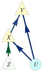<details> <summary>Image 12 Details</summary>  ### Visual Description ## Diagram: Directed Graph with Triangular and Circular Nodes ### Overview The image depicts a directed graph with four nodes: three triangular shapes (Y, X, Z) and one circular node (U). Arrows indicate directional relationships between nodes, with two colors (blue and green) distinguishing the connections. ### Components/Axes - **Nodes**: - **Y**: Yellow triangle at the top center. - **X**: Yellow triangle at the middle left. - **Z**: Gray triangle at the bottom left. - **U**: Light blue circle at the bottom right. - **Arrows**: - **Blue arrows**: - From Y to X (top to middle left). - From Y to U (top to bottom right). - **Green arrow**: - From X to Z (middle left to bottom left). - **No legend** is present to explicitly define arrow colors or node categories. ### Detailed Analysis - **Node Placement**: - Y is spatially dominant, positioned at the apex. - X and Z form a vertical alignment on the left side, with X above Z. - U is isolated on the right, receiving input only from Y. - **Directionality**: - Y → X and Y → U suggest Y as a source or influencer. - X → Z implies a downstream relationship from X to Z. - **Color Coding**: - Blue arrows may represent primary or direct relationships. - Green arrow (X → Z) could denote a secondary or specialized connection. ### Key Observations 1. **Central Role of Y**: Y is the only node with outgoing arrows to two other nodes (X and U), suggesting it acts as a hub or initiator. 2. **Isolation of U**: U has no outgoing arrows, indicating it may be a terminal or output node. 3. **Lack of Reciprocity**: No arrows point back to Y, X, or Z, implying a unidirectional flow. 4. **Color Ambiguity**: Without a legend, the significance of blue vs. green arrows remains speculative. ### Interpretation This diagram likely represents a hierarchical or causal system: - **Y** could symbolize a root cause, input, or primary variable influencing both **X** (a mediator) and **U** (an output). - **X**’s connection to **Z** might indicate a secondary process or dependency. - The absence of feedback loops suggests a linear or acyclic process. **Uncertainties**: - The purpose of node colors (yellow for triangles, gray for Z, light blue for U) is unclear. - Arrow colors lack explicit definitions, limiting interpretation of their functional significance. This structure could model workflows, decision trees, or dependency graphs in technical systems, though additional context is needed to confirm its application. </details> FIG. 12. The instrumental scenario of Pearl [31]. FIG. 13. An inflation of the instrumental scenario which illustrates why coinciding ancestral subgraphs doesn't necessarily imply coinciding marginal distributions. 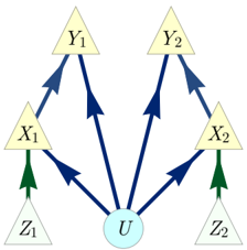<details> <summary>Image 13 Details</summary>  ### Visual Description ## Flowchart Diagram: System Architecture with Feedback Loops ### Overview The diagram illustrates a multi-node system architecture with directional relationships between components. It features a central node (U) connected to intermediate nodes (X1, X2), which in turn connect to terminal nodes (Z1, Z2) and feedback nodes (Y1, Y2). Arrows indicate directional flow or influence between components. ### Components/Axes - **Nodes**: - Central node: **U** (light blue circle) - Intermediate nodes: **X1** (left), **X2** (right) (yellow triangles) - Terminal nodes: **Z1** (bottom-left), **Z2** (bottom-right) (light green triangles) - Feedback nodes: **Y1** (top-left), **Y2** (top-right) (yellow triangles) - **Arrows**: - **Blue**: Connect U → X1/X2 and X1/X2 → Y1/Y2 - **Green**: Connect X1 → Z1 and X2 → Z2 - **Black**: Connect Y1/Y2 → X1/X2 (feedback loop) - **Legend**: No explicit legend present. Color coding appears to denote: - Blue: Primary flow - Green: Output/termination - Black: Feedback/recycling ### Detailed Analysis 1. **Primary Flow**: - U → X1 (blue arrow) - U → X2 (blue arrow) - X1 → Z1 (green arrow) - X2 → Z2 (green arrow) 2. **Feedback Mechanism**: - Y1 → X1 (black arrow) - Y2 → X2 (black arrow) 3. **Spatial Relationships**: - U is centrally positioned, acting as the system's origin. - X1/X2 form a bifurcation layer below U. - Z1/Z2 are terminal outputs at the lowest level. - Y1/Y2 are elevated feedback nodes above X1/X2. ### Key Observations - **Symmetry**: The system exhibits bilateral symmetry in its structure (left/right mirroring). - **Cyclical Dependency**: Feedback loops (Y1/Y2 → X1/X2) suggest iterative processes. - **Color Coding**: Blue arrows dominate (60% of connections), emphasizing their role as primary pathways. ### Interpretation This diagram likely represents a **closed-loop system** where: 1. **U** serves as the central processing unit or energy source. 2. **X1/X2** act as decision nodes or processing stages. 3. **Z1/Z2** represent final outputs or end states. 4. **Y1/Y2** function as monitoring/feedback mechanisms that regulate X1/X2 behavior. The absence of a legend introduces ambiguity about the significance of arrow colors, but the spatial arrangement strongly suggests: - **Top-down influence** from U to X1/X2 - **Bottom-up feedback** from Y1/Y2 to X1/X2 - **Divergent paths** to terminal states (Z1/Z2) The system may model processes like: - Resource allocation with feedback controls - Decision-making frameworks with iterative refinement - Biological/ecological systems with regulatory mechanisms Notably, the lack of quantitative values or time-based metrics limits analysis to structural interpretation. The diagram emphasizes **relational dynamics** over quantitative performance metrics. </details> FIG. 14. The ancestral subgraph of Fig. 13 for either { X 1 Y 2 Z 1 } or { X 1 Y 2 Z 2 } . 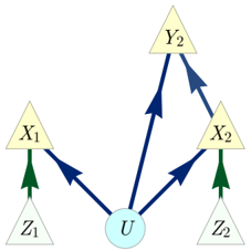<details> <summary>Image 14 Details</summary>  ### Visual Description ## Flowchart: System Process Diagram ### Overview The image depicts a flowchart with six nodes (X1, X2, Y2, Z1, Z2, U) and directional arrows. Arrows are color-coded (blue, green, dark blue) to indicate relationships or processes. The central node **U** acts as a hub connecting to other nodes. ### Components/Axes - **Nodes**: - **X1**, **X2**: Intermediate nodes connected to **U** via blue arrows. - **Y2**: Node connected to **X2** via a dark blue arrow. - **Z1**, **Z2**: Terminal nodes connected to **X1** and **X2** via green arrows, respectively. - **U**: Central node with bidirectional blue arrows to **X1** and **X2**. - **Arrows**: - **Blue**: Connect **U** to **X1**/**X2** (bidirectional). - **Green**: Connect **X1** to **Z1** and **X2** to **Z2** (unidirectional). - **Dark Blue**: Connect **Y2** to **X2** (unidirectional). - **No explicit legend**: Colors are embedded in the diagram without a separate key. ### Detailed Analysis - **Node U**: Central hub with bidirectional influence over **X1** and **X2**. - **X1**: Receives input from **U** and outputs to **Z1** via green arrow. - **X2**: Receives input from **U** and **Y2**, outputs to **Z2** via green arrow. - **Y2**: External input to **X2** via dark blue arrow, suggesting a secondary influence. - **Z1/Z2**: Terminal nodes with no outgoing arrows, indicating final outputs. ### Key Observations 1. **Centralized Control**: **U** governs the initial flow to **X1** and **X2**, implying a primary decision point. 2. **Divergent Paths**: **X1** and **X2** split into separate terminal nodes (**Z1**, **Z2**), suggesting parallel processes. 3. **Feedback Loop**: **Y2**’s connection to **X2** introduces an external input, potentially modifying the output to **Z2**. 4. **Color Coding**: Blue arrows (core connections), green arrows (outputs), and dark blue arrows (external inputs) differentiate relationship types. ### Interpretation The flowchart likely represents a system where **U** initiates processes that branch into **X1** and **X2**. These nodes then produce outputs (**Z1**, **Z2**), with **Y2** acting as an external modifier to **X2**. The use of color coding emphasizes the hierarchy of relationships: - **Blue** = Core bidirectional interactions (e.g., feedback between **U** and **X1/X2**). - **Green** = Terminal outputs (no further processing). - **Dark Blue** = External influence (e.g., **Y2** affecting **X2**). This structure could model decision trees, data flow in software, or cause-effect relationships in a technical system. The absence of numerical data suggests a conceptual rather than quantitative representation. </details> FIG. 15. Causal structure #15 in [22]. The d -separation relations are C ⊥ d Y and A ⊥ d B | Y . FIG. 16. Causal structure #16 in [22]. The only d -separation relation is C ⊥ d Y . 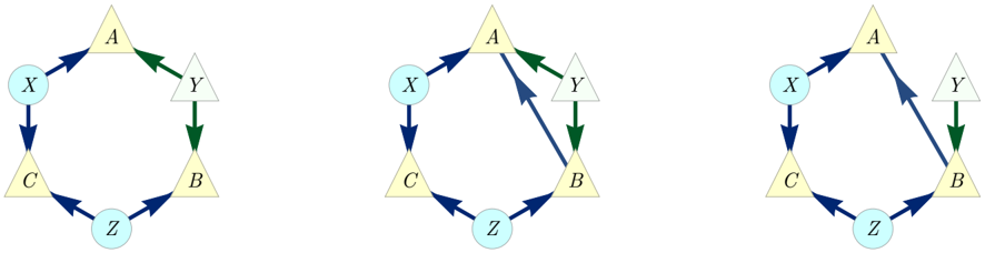<details> <summary>Image 15 Details</summary>  ### Visual Description ## Diagram: Node-Based Flow Structures (A, B, C) ### Overview The image presents three distinct diagrams (A, B, C) depicting node-based systems with directional arrows. Each diagram shares core nodes (X, A, Y, B, C, Z) but varies in connection patterns and arrow types. The diagrams use color-coded arrows (blue, green, black) to differentiate relationships, though no explicit legend is provided. ### Components/Axes - **Nodes**: - **X** (light blue circle) - **A** (yellow triangle) - **Y** (gray triangle) - **B** (yellow triangle) - **C** (yellow triangle) - **Z** (light blue circle) - **Arrows**: - **Blue**: Unidirectional flow (e.g., X → A, C → Z) - **Green**: Unidirectional flow (e.g., A → Y, Y → B) - **Black**: Bidirectional flow (e.g., A ↔ Y in Diagram B) - **Spatial Layout**: Nodes arranged in a circular pattern, with arrows connecting them in sequential or branching paths. ### Detailed Analysis #### Diagram A - **Flow Path**: X → A → Y → B → C → Z → X (closed loop). - **Key Connections**: - All arrows are unidirectional (blue/green). - No direct connection between X and Y or B and Z. #### Diagram B - **Flow Path**: X → A ↔ Y → B → C → Z → X (closed loop with bidirectional A-Y). - **Key Connections**: - Bidirectional arrow (black) between A and Y. - Maintains the closed loop structure but introduces mutual interaction between A and Y. #### Diagram C - **Flow Path**: X → B → C → Z → X (partial loop) and A → Y (isolated pair). - **Key Connections**: - Missing A-Y connection from Diagrams A/B. - Direct arrow (blue) from X to B, bypassing A. - A and Y form an isolated pair with no incoming/outgoing connections to the rest of the system. ### Key Observations 1. **Diagram A** represents a fully connected cycle with unidirectional flow. 2. **Diagram B** introduces a bidirectional relationship (A-Y), suggesting mutual dependency or feedback. 3. **Diagram C** disrupts the cycle, creating a fragmented system where A-Y operates independently, and X-B-Z form a smaller loop. ### Interpretation The diagrams likely model different network topologies or process flows: - **Diagram A** could represent a linear workflow with strict sequential dependencies. - **Diagram B** implies a system where certain components (A and Y) interact bidirectionally, enabling feedback or redundancy. - **Diagram C** suggests a hybrid structure where critical nodes (A, Y) are decoupled from the main flow, potentially indicating fault tolerance or modular design. **Uncertainties**: - The absence of a legend leaves the meaning of arrow colors open to interpretation (e.g., blue vs. green distinctions). - No numerical data or labels quantify the strength or frequency of connections, limiting quantitative analysis. **Peircean Insight**: The progression from A to C highlights how structural changes (e.g., adding/removing connections) alter system behavior. Diagram C’s isolation of A-Y might reflect a scenario where specific components are intentionally decoupled to test resilience or optimize resource allocation. </details> FIG. 17. Causal structure #20 in [22]. The d -separation relations are C ⊥ d Y and A ⊥ d Y | B . ## Appendix D: Using the Inflation Technique to Certify a Causal Structure as 'Interesting' By considering all possible d -separation relations on the observed nodes of a causal structure, one can infer the set of all conditional independence (CI) relations that must hold in any distribution compatible with it. Due to the presence of latent variables, satisfying these CI relations is generally not sufficient for compatibility. Henson, Lal and Pusey (HLP) [22] introduced the term interesting for those causal structures for which this happens, and derived a partial classification of causal structures into interesting and non-interesting ones by finding necessary criteria for a causal structure to be interesting, and they also conjectured their criteria to be sufficient. As evidence in favour of this conjecture, they enumerated all possible isomorphism classes of causal structure with up to six nodes satisfying their criteria, which resulted in only 21 equivalence classes of potentially interesting causal structures. Of those 21, they further proved that 18 were indeed interesting by writing down explicit distributions which are incompatible despite satisfying the observed CI relations. Incompatibility was certified by means of entropic inequalities. That left three classes of causal structures as potentially interesting. For each of these, HLP derived both: (i) the set of Shannon-type entropic inequalities that take into account the CI relations among the observed variables, and (ii) the set of Shannon-type entropic inequalities that also take into account CI relations among latent variables. Finding the second set to be larger than the first constitutes evidence that the causal structure is interesting. The evidence is not conclusive, however, because the Shannon-type inequalities that are included in the second set but not the first might be non-Shannon-type inequalities that merely follow from the CI relations among the observed variables [22]. One way to close this loophole would be to show that the novel Shannon-type inequalities imply constraints beyond some inner approximation to the genuine entropic cone corresponding to the CI relations among observed variables, perhaps along the lines of [26]. Another is to use causal compatibility inequalities beyond entropic inequalities to identify some CI-respecting but incompatible distributions. Pienaar [36] accomplished precisely this by considering the different values that an observed root variable may take. In the following, we demonstrate how the inflation technique can be used for the same purpose. ## 1. Certifying that Henson-Lal-Pusey's Causal Structure #16 is 'Interesting' Pienaar [36] identified a distribution which satisfies the only CI relation that must hold among the observed variables in HLP's causal structure #16 (Fig. 16 here), namely, C ⊥ ⊥ Y , but which is nonetheless incompatible with it: $$P _ { A B C Y } ^ { P i e n a a r } \colon = \frac { [ 0 0 0 0 ] + [ 0 1 1 0 ] + [ 0 0 0 1 ] + [ 1 0 1 1 ] } { 4 } , \quad \text {i.e.,} \quad P _ { A B C Y } ^ { P i e n a a r } ( a b c y ) = \begin{cases} \frac { 1 } { 4 } & \text {if $y\cdot c=a$ and $(y\oplus 1)\cdot c=b$,} \\ 0 & \text {otherwise.} \end{cases}$$ It is useful to compute the conditional on Y , $$P _ { A B C | Y } ^ { P i e n a r } ( \cdots | y ) = \begin{cases} \frac { 1 } { 2 } ( [ 0 0 0 ] + [ 0 1 1 ] ) & \text {if $y=0$,} \\ \frac { 1 } { 2 } ( [ 0 0 0 ] + [ 1 0 1 ] ) & \text {if $y=1$.} \end{cases}$$ This makes it evident that the distribution can be described as follows: if Y = 0, then A = 0 while B and C are FIG. 18. The Russian dolls inflation of Fig. 16. 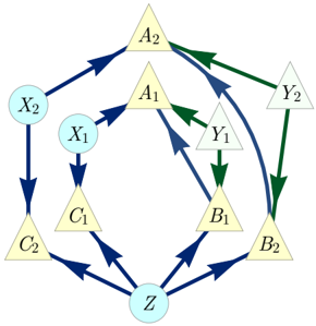<details> <summary>Image 16 Details</summary>  ### Visual Description ## Flowchart Diagram: System Process Flow ### Overview The image depicts a directed flowchart with 11 nodes (labeled A1, A2, B1, B2, C1, C2, X1, X2, Y1, Y2, Z) and 12 directed edges. The diagram uses three arrow colors (blue, green, dark blue) to distinguish connection types. The structure suggests a multi-stage process with feedback loops and branching pathways. ### Components/Axes - **Nodes**: - Central node: Z (light blue circle) - Intermediate nodes: C1, C2 (yellow triangles), A1, A2, B1, B2 (yellow triangles) - Terminal nodes: X1, X2, Y1, Y2 (light blue circles) - **Edges**: - **Blue arrows**: Primary connections (e.g., Z→C1, C1→A1) - **Green arrows**: Secondary connections (e.g., A1→A2, B1→B2) - **Dark blue arrows**: Feedback/loop connections (e.g., A2→A1) - **Spatial Layout**: - Bottom: Z (central hub) - Middle: C1/C2 (left/right branches) - Top: A1/A2 (left), B1/B2 (right) - Right: Y1/Y2 (output cluster) - Loop: A2→A1 (right-side feedback) ### Detailed Analysis 1. **Node Connections**: - **Z** (bottom center) → C1 (blue) and C2 (blue) - **C1** → A1 (blue) and X1 (dark blue) - **C2** → B1 (blue) and X2 (dark blue) - **A1** → A2 (green) and Y1 (dark blue) - **B1** → B2 (green) and Y2 (dark blue) - **A2** → A1 (dark blue, feedback loop) - **B2** → Y2 (dark blue, terminal) - **Y1/Y2** have no outgoing edges (final outputs) 2. **Color-Coded Relationships**: - **Blue**: Core process flow (80% of connections) - **Green**: Secondary/optional pathways (2 connections) - **Dark Blue**: Feedback/termination (3 connections) ### Key Observations - **Feedback Loop**: A2→A1 creates a cyclical dependency, suggesting iterative refinement or error correction. - **Divergent Paths**: C1 and C2 split into A1/B1 branches, indicating parallel processing streams. - **Convergence**: Y1/Y2 act as terminal nodes, possibly representing final outputs or decision points. - **X1/X2**: Isolated nodes with only incoming dark blue arrows, potentially representing error states or dead ends. ### Interpretation This diagram likely models a **multi-stage decision-making system** with: 1. **Input Stage**: Z (central resource) feeds into two parallel processes (C1/C2). 2. **Processing Streams**: - **A-path**: C1→A1→A2 (with feedback to A1) - **B-path**: C2→B1→B2 (linear progression) 3. **Output Stage**: Y1/Y2 as final results, with X1/X2 as potential failure states. 4. **Regulatory Mechanism**: The A2→A1 loop implies self-correction or iterative optimization. The color coding emphasizes **process hierarchy** (blue > green > dark blue), while the spatial layout separates input, processing, and output phases. The feedback loop in the A-path suggests a focus on refinement, whereas the B-path represents a more linear workflow. X1/X2 may indicate system vulnerabilities or termination points requiring further analysis. </details> uniformly random and perfectly correlated, while if Y = 1, then B = 0 and A and C are uniformly random and perfectly correlated. Here, we will establish the incompatibility of Pienaar's distribution with HLP's causal structure #16 (Fig. 16 here) using the inflation technique. To do so, we use the inflation depicted in Fig. 18, which we term the Russian dolls inflation. We will make use of the fact that { A 1 C 1 Y 1 } , { B 2 C 2 Y 2 } and { B 2 C 1 Y 2 } are injectable sets, together with the fact that { A 1 C 2 Y 1 } is an expressible set. We begin by demonstrating how the d -separation relations in the Russian dolls inflation imply that { A 1 C 2 Y 1 } is expressible. First, we note that the set { A 1 B 1 C 2 Y 1 } is expressible because the d -separation relation A 1 ⊥ d C 2 | B 1 Y 1 implies that $$P _ { A _ { 1 } B _ { 1 } C _ { 2 } Y _ { 1 } } = \frac { P _ { A _ { 1 } B _ { 1 } Y _ { 1 } } P _ { C _ { 2 } B _ { 1 } Y _ { 1 } } } { P _ { B _ { 1 } Y _ { 1 } } } , & & ( D . 3 )$$ and the sets { A 1 B 1 Y 1 } , { C 2 B 1 Y 1 } , and { B 1 Y 1 } are injectable. The expressibility of { A 1 C 2 Y 1 } then follows from the expressibility of { A 1 B 1 C 2 Y 1 } and the fact that the distribution on the former can be obtained from the distribution on the latter by marginalization, $$P _ { A _ { 1 } C _ { 2 } Y _ { 1 } } ( a c y ) = \sum _ { b } P _ { A _ { 1 } B _ { 1 } C _ { 2 } Y _ { 1 } } ( a b c y ) .$$ It follows that the distribution P A 1 C 2 Y 1 in the inflation model associated to the Pienaar distribution can be computed by first writing down the distributions on the relevant injectable sets, $$P _ { B _ { 2 } C _ { 2 } Y _ { 2 } } ( b c y ) & = P ^ { \text {Pienaar} } _ { B C Y } ( b c y ) , \\ P _ { A _ { 1 } C _ { 1 } Y _ { 1 } } ( a c y ) & = P ^ { \text {Pienaar} } _ { A C Y } ( a c y ) , & & ( D . 5 )$$ and from Eq. (D.4) and (D.3), as well as the injectability of { A 1 B 1 Y 1 } , { C 2 B 1 Y 1 } , and { B 1 Y 1 } , we infer that $$P _ { A _ { 1 } C _ { 2 } Y _ { 1 } } ( a c y ) = \sum _ { b } \frac { P ^ { P i e n a r } _ { A B Y } ( a b y ) P ^ { P i e n a r } _ { C B Y } ( c b y ) } { P ^ { P i e n a r } _ { B Y } ( b y ) } .$$ We are now in a position to derive a contradiction. Our derivation will begin by setting Y 2 = 0 and Y 1 = 1. It is therefore convenient to condition on Y 1 and Y 2 in the distributions of interest and set them equal to these values, and to express these in terms of the conditioned Pienaar distribution via Eq. (D.5), $$P _ { B _ { 2 } C _ { 2 } | Y _ { 2 } } ( b c | 0 ) & = P ^ { \text {Pienaar} } _ { B C | Y } ( b c | 0 ) \\ P _ { A _ { 1 } C _ { 1 } | Y _ { 1 } } ( a c | 1 ) & = P ^ { \text {Pienaar} } _ { A C | Y } ( a c | 1 ) \\ P _ { B _ { 2 } C _ { 1 } | Y _ { 2 } } ( b c | 0 ) & = P ^ { \text {Pienaar} } _ { B C | Y } ( b c | 0 )$$ and similarly from Eq. (D.6), $$P _ { A _ { 1 } C _ { 2 } | Y _ { 1 } } ( a c | 1 ) = \sum _ { b } \frac { P ^ { P i e n a a r } _ { A B | Y } ( a b | 1 ) P ^ { P i e n a a r } _ { C B | Y } ( c b | 1 ) } { P ^ { P i e n a a r } _ { B | Y } ( b | 1 ) } .$$ From these and Eq. (D.2), we infer $$P _ { B _ { 2 } C _ { 2 } | Y _ { 2 } } ( \cdot \cdot | 0 ) = \frac { 1 } { 2 } ( [ 0 0 ] + [ 1 1 ] ) , & & ( D . 9 )$$ $$P _ { A _ { 1 } C _ { 1 } | Y _ { 1 } } ( \cdots | 1 ) = \frac { 1 } { 2 } ( [ 0 0 ] + [ 1 1 ] ) ,$$ $$P _ { B _ { 2 } C _ { 1 } | Y _ { 2 } } ( \cdots | 0 ) = \frac { 1 } { 2 } ( [ 0 0 ] + [ 1 1 ] ) , & & ( D . 1 1 )$$ $$P _ { A _ { 1 } C _ { 2 } | Y _ { 1 } } ( \cdot \cdot | 1 ) = \frac { 1 } { 4 } ( [ 0 0 ] + [ 0 1 ] + [ 1 0 ] + [ 1 1 ] ) .$$ Henceforth, we leave the condition that Y 2 = 0 and Y 1 = 1 implicit. From Eq. (D.11), we have $$\text {With probability } 1 / 2 , B _ { 2 } = 0 \, \text {and} \, C _ { 1 } = 0 .$$ From Eq. (D.9), we have $$\text {If $B_{2}=0$ then $C_{2} = 0$.}$$ From Eq. (D.10), we have $$\text {If $C_{1}=0$ then $A_{1} = 0$.}$$ These three statements imply that The probability that C = 0 and A = 0 is ≥ 1 / 2 . $$\text {probability that} \, C _ { 2 } = 0 \text { and } A _ { 1 } = 0 \text { is } \geq 1 / 2 .$$ However, Eq. (D.12) implies that the probability of C 2 = 0 and A 1 = 0 is only p = 1 / 4. We have therefore arrived at a contradiction. This establishes the incompatibility of the Pienaar distribution with HLP's causal structure #16. Our reasoning is again a form of the Hardy-type arguments from Sec. IV D. ## 2. Deriving a Causal Compatibility Inequality for HLP's Causal Structure #16 We can also turn the above argument into an inequality. Using the methods of Sec. IV D, it is straightforward to show that the assumption of a joint distribution on { A 1 B 2 C 1 Y 1 Y 2 } implies the inequality on marginals, $$P _ { B _ { 2 } C _ { 1 } Y _ { 1 } Y _ { 2 } } ( 0 0 1 0 ) \leq P _ { B _ { 2 } C _ { 2 } Y _ { 1 } Y _ { 2 } } ( 0 1 1 0 ) + P _ { A _ { 1 } C _ { 1 } Y _ { 1 } Y _ { 2 } } ( 1 0 1 0 ) + P _ { A _ { 1 } C _ { 2 } Y _ { 1 } Y _ { 2 } } ( 0 0 1 0 ) .$$ From the following four ancestral independences in the inflated causal structure, B 2 C 1 Y 2 ⊥ d Y 1 , B 2 C 2 Y 2 ⊥ d Y 1 , A 1 C 1 Y 1 ⊥ d Y 2 , and A 1 C 2 Y 1 ⊥ d Y 2 , we infer, respectively, the following factorization conditions: $$P _ { B _ { 2 } C _ { 1 } Y _ { 2 } Y _ { 1 } } & = P _ { B _ { 2 } C _ { 1 } Y _ { 2 } } P _ { Y _ { 1 } } , \\ P _ { B _ { 2 } C _ { 2 } Y _ { 2 } Y _ { 1 } } & = P _ { B _ { 2 } C _ { 2 } Y _ { 2 } } P _ { Y _ { 1 } } , \\ P _ { A _ { 1 } C _ { 1 } Y _ { 1 } Y _ { 2 } } & = P _ { A _ { 1 } C _ { 1 } Y _ { 1 } } P _ { Y _ { 2 } } , \\ P _ { A _ { 1 } C _ { 2 } Y _ { 1 } Y _ { 2 } } & = P _ { A _ { 1 } C _ { 2 } Y _ { 1 } } P _ { Y _ { 2 } } . P _ { B _ { 2 } C _ { 1 } Y _ { 2 } Y _ { 1 } } & = P _ { B _ { 2 } C _ { 1 } Y _ { 2 } } P _ { Y _ { 1 } } , \\ P _ { B _ { 2 } C _ { 2 } Y _ { 2 } Y _ { 1 } } & = P _ { B _ { 2 } C _ { 2 } Y _ { 2 } } P _ { Y _ { 1 } } , \\ P _ { A _ { 1 } C _ { 1 } Y _ { 1 } Y _ { 2 } } & = P _ { A _ { 1 } C _ { 1 } Y _ { 1 } } P _ { Y _ { 2 } } , \\ P _ { A _ { 1 } C _ { 2 } Y _ { 1 } Y _ { 2 } } & = P _ { A _ { 1 } C _ { 2 } Y _ { 1 } } P _ { Y _ { 2 } } . P _ { B _ { 2 } C _ { 1 } Y _ { 2 } Y _ { 1 } } & = P _ { B _ { 2 } C _ { 1 } Y _ { 2 } } P _ { Y _ { 1 } } , \\ P _ { B _ { 2 } C _ { 2 } Y _ { 2 } Y _ { 1 } } & = P _ { B _ { 2 } C _ { 2 } Y _ { 2 } } P _ { Y _ { 1 } } , \\ P _ { A _ { 1 } C _ { 1 } Y _ { 1 } Y _ { 2 } } & = P _ { A _ { 1 } C _ { 1 } Y _ { 1 } } P _ { Y _ { 2 } } , \\ P _ { A _ { 1 } C _ { 2 } Y _ { 1 } Y _ { 2 } } & = P _ { A _ { 1 } C _ { 2 } Y _ { 1 } } P _ { Y _ { 2 } } .$$ Substituting these into Eq. (D.17), we obtain: $$P _ { B _ { 2 } C _ { 1 } Y _ { 2 } } ( 0 0 0 ) P _ { Y _ { 1 } } ( 1 ) \leq P _ { B _ { 2 } C _ { 2 } Y _ { 2 } } ( 0 1 0 ) P _ { Y _ { 1 } } ( 1 ) + P _ { A _ { 1 } C _ { 1 } Y _ { 1 } } ( 1 0 1 ) P _ { Y _ { 2 } } ( 0 ) + P _ { A _ { 1 } C _ { 2 } Y _ { 1 } } ( 0 0 1 ) P _ { Y _ { 2 } } ( 0 ) .$$ This is a nontrivial causal compatibility inequality for the inflated causal structure. However, in this form, it cannot be translated into one for the observed variables in the original causal structure: the sets { B 2 C 1 Y 2 } , { B 2 C 2 Y 2 } and { A 1 C 1 Y 1 } are injectable, and the singleton sets { Y 1 } and { Y 2 } are injectable (by the definition of inflation), the set { A 1 C 2 Y 1 } is merely expressible. Therefore, we must substitute the expression for P A 1 C 2 Y 1 given by Eqs. (D.3,D.4) into Eq. (D.19), to obtain $$P _ { B _ { 2 } C _ { 1 } Y _ { 2 } } ( 0 0 0 ) P _ { Y _ { 1 } } ( 1 ) & \leq P _ { B _ { 2 } C _ { 2 } Y _ { 2 } } ( 0 1 0 ) P _ { Y _ { 1 } } ( 1 ) + P _ { A _ { 1 } C _ { 1 } Y _ { 1 } } ( 1 0 1 ) P _ { Y _ { 2 } } ( 0 ) + \sum _ { b } \frac { P _ { A _ { 1 } B _ { 1 } Y _ { 1 } } ( 0 b 1 ) P _ { B _ { 1 } C _ { 2 } Y _ { 1 } } ( 0 b 1 ) } { P _ { B _ { 1 } Y _ { 1 } } ( b 1 ) } P _ { Y _ { 2 } } ( 0 ) .$$ This is also a nontrivial causal compatibility inequality for the inflated causal structure, but now it refers exclusively to distributions on injectable sets. As such, we can directly translate it into a nontrivial causal compatibility inequality for the original causal structure, namely, <!-- formula-not-decoded --> Dividing by P Y (0) P Y (1), and using the definition of conditional probabilities, this inequality can be expressed in the form $$P _ { B C | Y } ( 0 0 | 0 ) \leq P _ { B C | Y } ( 0 1 | 0 ) + P _ { A C | Y } ( 1 0 | 1 ) + \sum _ { b } \frac { P _ { A B | Y } ( 0 b | 1 ) P _ { B C | Y } ( 0 b | 1 ) } { P _ { B | Y } ( b | 1 ) } .$$ This inequality is strong enough to witness the incompatibility of Pienaar's distribution Eq. (D.1) with HLP's causal structure #16. ## 3. Certifying that Henson-Lal-Pusey's Causal Structures #15 and #20 are 'Interesting' Any distribution P ABCY that is incompatible with HLP's causal structure #16 is also incompatible with HLP's causal structures #15 (Fig. 15 here) and #20 (Fig. 17 here) because the causal models defined by HLP's causal structures #15 and #20 are included among the causal models defined by HLP's causal structure #16 (Fig. 16 here). Consequently, Eq. (D.22) is also a valid causal compatibility inequality for HLP's causal structure #15 and for HLP's causal structure #20. It follows that if one can find a distribution that exhibits all of the observable CI relations implied by either of HLP's causal structures #15 and #20, namely, C ⊥ ⊥ Y (per #15 and #16), A ⊥ ⊥ B | Y (per #15), and A ⊥ ⊥ Y | B (per #20), and which moreover is not compatible with HLP's causal structure #16, then this proves-in one go-that HLP's causal structures #15, #16 and #20 are interesting. Any distribution P ABCY with the conditional 37 $$P _ { A B C | Y } ( a b c | y ) \colon = & \begin{cases} \frac { 1 } { 4 } ( [ 0 0 0 ] + [ 1 1 1 ] + [ 0 1 1 ] + [ 1 0 0 ] ) & \text {if $y=0$,} \\ \frac { 1 } { 4 } ( [ 0 0 0 ] + [ 1 1 1 ] + [ 0 1 0 ] + [ 1 0 1 ] ) & \text {if $y=1$,} \end{cases}$$ achieves this because it satisfies the required CI relations while also violating Eq. (D.22). 37 We take the definition of the conditional P ABC | Y from the distribution P ABCY as also implying P Y (0) > 0 and P Y (1) > 0. ## Appendix E: The Copy Lemma and Non-Shannon type Entropic Inequalities The inflation technique may also be useful outside beyond causal inference. As we argue in the following, inflation is secretly what underlies the Copy Lemma in the derivation of non-Shannon type entropic inequalities [119, Chapter 15]. The following formulation of the Copy Lemma is the one of Kaced [120]. Lemma 12. Let A , B and C be random variables with joint distribution P ABC . Then there exists a fourth random variable A ′ and joint distribution P AA ′ BC such that: 1. P AB = P A ′ B , 2. A ′ ⊥ ⊥ AC | B . The proof via inflation is as follows. Proof. Every joint distribution P ABC is compatible with the causal structure of Fig. 19. This follows from the fact that one may take X to be any sufficient statistic for the joint variable ( A,C ) given B , such as X := ( A,B,C ). Next, we consider the inflation of Fig. 19 depicted in Fig. 20. The maximal injectable sets are { A 1 B 1 C 1 } and { A 2 B 1 } . By Lemma 4, because P ABC is assumed to be compatible with Fig. 19, it follows that the family of marginals { P A 1 B 1 C 1 , P A 2 B 1 } , where P A 1 B 1 C 1 := P ABC and P A 2 B 1 := P AB , is compatible with the inflation of Fig. 20. The resulting joint distribution P A 1 A 2 B 1 C 1 has marginals P A 1 B 1 = P A 2 B 1 = P AB and satisfies the conditional independence relation A 2 ⊥ ⊥ A 1 C 1 | B 1 , since A 2 is d -separated from A 1 C 1 by B 1 in Fig. 20. While it is also not hard to write down the distribution constructed in the proof explicitly as P A 1 A 2 B 1 C 1 := P A 1 B 1 C 1 P A 2 B 1 P -1 B 1 [119, Lemma 15.8], the fact that one can reinterpret it using the inflation technique is significant. For one, all the non-Shannon type inequalities derived by Dougherty et al. [121] are obtained by applying some Shannon-type inequality to the distribution derived from the Copy Lemma. Our result shows, therefore, that one can understand these non-Shannon type inequalities for a causal structure as arising from Shannon-type inequalities applied to an inflated causal structure. We thus speculate that the inflation technique may be a more general-purpose tool for deriving non-Shannon-type entropic inequalities. A natural direction for future research is to explore whether more sophisticated applications of the inflation technique might result in new examples of such inequalities. FIG. 19. A causal structure that is compatible with any distribution P ABC . 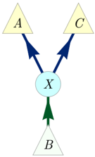<details> <summary>Image 17 Details</summary>  ### Visual Description ## Diagram: Triangular Node Network with Central Hub ### Overview The diagram depicts a network of three triangular nodes (A, C, B) connected to a central circular node (X). Arrows indicate directional relationships: two blue arrows point from A and C to X, and one green arrow points from X to B. No numerical data, scales, or legends are present. ### Components/Axes - **Nodes**: - **A**: Top-left triangle (yellow fill). - **C**: Top-right triangle (yellow fill). - **B**: Bottom triangle (light green fill). - **X**: Central circle (light blue fill). - **Arrows**: - **Blue arrows**: Connect A→X and C→X. - **Green arrow**: Connects X→B. - **No axis titles, legends, or numerical markers** are visible. ### Detailed Analysis - **Textual Labels**: - All nodes are labeled with uppercase letters (A, C, B, X). - No additional text, annotations, or legends are present. - **Spatial Relationships**: - A and C are positioned symmetrically above X. - B is directly below X, aligned vertically. - Arrows are straight and unambiguous in direction. ### Key Observations 1. **Directional Flow**: - Inputs from A and C converge at X. - Output from X is directed to B. 2. **Color Coding**: - Blue arrows (A→X, C→X) may imply a shared process or relationship. - Green arrow (X→B) suggests a distinct or prioritized pathway. 3. **Symmetry**: - A and C are equidistant from X, suggesting equal influence or input. ### Interpretation The diagram likely represents a system where: - **X acts as a central processor or hub**, receiving inputs from A and C and transmitting output to B. - The **color differentiation** (blue vs. green arrows) could indicate: - **Blue**: Standard or primary relationships (A and C → X). - **Green**: A specialized or secondary relationship (X → B). - **Symmetry** between A and C implies they play equivalent roles in the network. **Notable Patterns**: - No feedback loops or bidirectional relationships are depicted. - The absence of numerical data limits quantitative analysis; the focus is on structural relationships. **Underlying Implications**: - This could model a decision-making process, data flow in a system, or hierarchical organization. - The green arrow’s uniqueness (X→B) might highlight B as a critical output or endpoint. </details> FIG. 20. An inflation of Fig. 19. 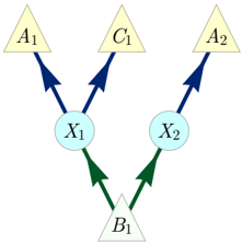<details> <summary>Image 18 Details</summary>  ### Visual Description ## Diagram: Node-Based System Architecture ### Overview The diagram illustrates a node-based system with directional relationships between components. It features six labeled nodes (A1, C1, A2, X1, X2, B1) connected by colored arrows (blue and green). The structure suggests a flow of information or processes from input nodes to intermediate nodes and finally to an output node. ### Components/Axes - **Nodes**: - **A1, C1, A2**: Positioned at the top, likely representing input or source components. - **X1, X2**: Intermediate nodes in the middle layer. - **B1**: Final output node at the bottom. - **Arrows**: - **Blue arrows**: Connect A1 → X1, C1 → X1, and X2 → A2. - **Green arrows**: Connect X1 → B1 and X2 → B1. - **Color Coding**: - Blue arrows may represent primary input pathways. - Green arrows may represent final processing or output pathways. ### Detailed Analysis 1. **Input Nodes (A1, C1, A2)**: - A1 and C1 both connect to X1 via blue arrows, suggesting they contribute to the same intermediate process (X1). - A2 connects to X2 via a blue arrow, indicating a separate input pathway for X2. 2. **Intermediate Nodes (X1, X2)**: - X1 receives inputs from A1 and C1, then outputs to B1 via a green arrow. - X2 receives input from A2 and outputs to B1 via a green arrow. 3. **Output Node (B1)**: - B1 aggregates inputs from both X1 and X2, acting as the terminal node. ### Key Observations - **Flow Direction**: All arrows point downward, indicating a unidirectional flow from top (inputs) to bottom (output). - **Symmetry**: X1 and X2 have identical roles (receiving inputs and outputting to B1), but their input sources differ (A1/C1 vs. A2). - **Color Consistency**: Blue arrows dominate the input layer, while green arrows dominate the output layer, reinforcing functional separation. ### Interpretation This diagram likely represents a **workflow or system architecture** where: - **A1, C1, and A2** are independent input sources or processes. - **X1 and X2** act as processing units that consolidate inputs before passing results to **B1**, the final output. - The use of distinct arrow colors (blue for inputs, green for outputs) emphasizes modularity and separation of concerns. The absence of numerical data or explicit labels for relationships suggests the diagram focuses on **structural relationships** rather than quantitative metrics. The symmetry between X1 and X2 implies redundancy or parallel processing capabilities in the system. </details> ## Appendix F: Causal Compatibility Inequalities for the Triangle Scenario in Machine-Readable Format Table II lists the fifty two numerically irredundant polynomial inequalities resulting from consistent marginals of the Spiral inflation of Fig. 3. Stronger inequalities can be derived be considering larger inflations, such as the Web inflation of Fig. 2. Each row in the table specifies the coefficient of the corresponding correlator monomial. As noted previously, these inequalities also follow from the hypergraph transversals technique per Sec. IV D. TABLE II. A machine-readable and closed-under-symmetries version of the table in Sec. IV C. | constant | E [ A ] | E [ B | E [ C ] | E [ AB ] | E [ AC | ] E [ BC ] | E [ ABC ] | E [ A ] E [ B | E [ A ] E [ C | ] E [ B ] E [ C ] | E [ A ] E [ BC ] | E [ AC ] E [ B ] | E [ AB ] E [ C | E [ A ] E [ B ] E [ C | |------------|-----------|---------|-----------|------------|----------|--------------|-------------|-----------------|-----------------|---------------------|--------------------|--------------------|------------------|-------------------------| | 1 | 0 | 0 | 0 | -1 | -1 | 0 | 0 | 0 | 0 | 1 | 0 | 0 | 0 | 0 | | 1 | 0 | 0 | 0 | -1 | 1 | 0 | 0 | 0 | 0 | -1 | 0 | 0 | 0 | 0 | | 1 | 0 | 0 | 0 | 1 | -1 | 0 | 0 | 0 | 0 | -1 | 0 | 0 | 0 0 | 0 | | 1 | 0 | 0 | 0 | 1 | 1 | 0 | 0 0 | 0 0 | 0 1 | 1 0 | 0 | 0 0 | 0 | 0 | | 1 1 | 0 0 | 0 0 | 0 0 | -1 -1 | 0 0 | -1 1 | 0 | 0 | -1 | 0 | 0 0 | 0 | 0 | 0 0 | | 1 | 0 | | | | | -1 | 0 | 0 | -1 | 0 | 0 | 0 | 0 | 0 | | 1 | 0 | 0 0 | 0 0 | 1 1 | 0 0 | 1 | 0 | 0 | 1 | 0 | 0 | 0 | 0 | 0 | | 1 | 0 | 0 | 0 | 0 | -1 | -1 | 0 | 1 | 0 | 0 | 0 | 0 | 0 | 0 | | 1 | 0 | 0 | 0 | 0 | -1 | 1 | 0 | -1 | 0 | 0 | 0 | 0 | 0 | 0 | | 1 | 0 | 0 | 0 | 0 | 1 | -1 | 0 | -1 | 0 | 0 | 0 | 0 | 0 | 0 | | 1 | 0 | 0 | 0 | 0 | 1 | 1 | 0 | 1 | 0 | 0 | 0 | 0 | 0 | 0 | | 3 | -1 | -1 | -1 | 2 | 2 | 2 | 1 | 1 | 1 | 1 | -1 | -1 | -1 | 1 | | 3 | -1 | -1 | 1 | 2 | -2 | -2 | -1 | 1 | -1 | -1 | 1 | 1 | 1 | -1 | | 3 | -1 | | | -2 | 2 | | -1 | | | -1 | 1 | 1 | 1 | -1 | | | | 1 | -1 | | | -2 | | -1 | 1 | | | | | | | 3 | 1 | -1 | -1 | -2 | -2 | 2 | -1 | -1 | -1 | 1 | 1 | 1 | 1 | -1 | | 3 | 1 | -1 | 1 | -2 | 2 | -2 | 1 | -1 | 1 | -1 | -1 | -1 | -1 | 1 | | 3 | 1 | 1 | -1 | 2 | -2 | -2 | 1 | 1 | -1 | -1 | -1 | -1 | -1 | 1 | | 3 4 | 1 -2 | 1 0 | 1 0 | 2 -3 | 2 -2 | 2 -2 | -1 1 | 1 1 | 1 0 | 1 2 | 1 1 | 1 1 | 1 0 | -1 -1 | | 4 | -2 | 0 | 0 | -3 | 2 | 2 | -1 | 1 | 0 | -2 | -1 | -1 | 0 | 1 | | 4 | -2 | 0 | 0 | 3 | -2 | 2 | -1 | -1 | 0 | -2 | -1 | -1 | 0 | 1 | | 4 | -2 | 0 | 0 | 3 | 2 | -2 | 1 | -1 | 0 | 2 | 1 | 1 | 0 | -1 | | 4 | 2 | 0 | 0 | -3 | -2 | -2 | -1 | 1 | 0 | 2 | -1 | -1 | 0 | 1 | | 4 | 2 | 0 | 0 | -3 | 2 | 2 | 1 | 1 | 0 | -2 | 1 | 1 | 0 | -1 | | 4 | 2 | 0 | 0 | 3 | -2 | 2 | 1 | -1 | 0 | -2 | 1 | 1 | 0 | -1 | | 4 | 2 | 0 | 0 | 3 | 2 | -2 | -1 | -1 | 0 | 2 | -1 | -1 | 0 | 1 | | 4 | 0 | -2 | 0 | -2 | -2 | -3 | 1 | 0 | 2 | 1 | 0 | 1 | 1 | -1 | | 4 | 0 | -2 | 0 | -2 | 2 | 3 | -1 | 0 | -2 2 | -1 -1 | 0 | -1 | -1 | 1 | | 4 4 | 0 0 | -2 -2 | 0 0 | 2 2 | -2 2 | 3 -3 | 1 -1 | 0 0 | -2 | 1 | 0 0 | 1 -1 | 1 -1 | -1 1 | | 4 | 0 | 2 | 0 | -2 | -2 | -3 | -1 | 0 | 2 | 1 | 0 | -1 | -1 | 1 | | | | 2 | | | 2 | | | | | | 0 | 1 | | | | 4 | 0 | | 0 | -2 | | 3 | 1 | 0 | -2 | -1 | | | 1 | -1 | | 4 4 | 0 0 | 2 2 | 0 0 | 2 | -2 | 3 | -1 1 | 0 0 | 2 -2 | -1 1 | 0 0 | -1 1 | -1 1 | 1 -1 | | 4 | 0 | 0 | -2 | 2 -2 | 2 -3 | -3 -2 | 1 | 2 | 1 | 0 | 1 | 0 | 1 | -1 | | 4 | 0 | 0 | -2 | | 3 | | 1 | 2 | -1 | 0 | 1 | 0 | 1 | -1 | | 4 | 0 | 0 | -2 | -2 2 | -3 | 2 2 | -1 | -2 | 1 | 0 | -1 | 0 | -1 | 1 | | 4 | 0 | 0 | -2 | 2 | 3 | -2 | | -2 | -1 | 0 | -1 | 0 | -1 | 1 | | 4 | 0 | 0 | 2 | -2 | -3 | -2 | -1 | 2 | 1 | 0 | -1 | 0 | -1 | 1 | | 4 | 0 | 0 | 2 | -2 | 3 | | -1 | 2 | -1 | 0 | -1 | 0 | | | | 4 | 0 | 0 | 2 | 2 | -3 | 2 | -1 | -2 | 1 | 0 | 1 | 0 | -1 1 | 1 | | 4 | 0 | 0 | 2 | 2 | 3 | 2 -2 | 1 1 | -2 | -1 | 0 | 1 | 0 | 1 | -1 -1 | | 4 | 0 | 0 | 0 | -2 | -2 | -2 | -1 | 2 | 2 | 2 | -1 | -1 | -1 | 0 | | 4 | | | | | | | | | | | 1 | 1 | 1 | | | | 0 | 0 | 0 | -2 | -2 | -2 | 1 | 2 | 2 | 2 | | | | 0 | | 4 4 | 0 0 | 0 0 | 0 0 | -2 -2 | 2 2 | 2 2 | -1 1 | 2 2 | -2 -2 | -2 -2 | -1 | -1 1 | -1 1 | 0 0 | | | | | | 2 | -2 | | -1 | -2 | 2 | -2 | 1 -1 | -1 | -1 | 0 | | 4 | 0 | 0 | 0 | 2 | | 2 | | -2 | | | 1 | | | 0 | | 4 | 0 | 0 | 0 | | -2 | 2 | 1 | | 2 | -2 | | 1 | 1 | | | 4 4 | 0 0 | 0 0 | 0 0 | 2 2 | 2 2 | -2 -2 | -1 1 | -2 -2 | -2 -2 | 2 2 | -1 1 | -1 1 | -1 1 | 0 0 | ## Appendix G: Recovering the Bell Inequalities from the Inflation Technique To further illustrate the power of the inflation technique, we now demonstrate how to recover all Bell inequalities [18, 20, 51] via our method. To keep things simple we only discuss the case of a bipartite Bell scenario with two values for both 'settings' and 'outcome' variables, but the case of more parties and/or more values per settings or outcome variable is totally analogous. The causal structure associated to the Bell [17, 18, 20, 51] scenario [22 (Fig. E#2), 19 (Fig. 19), 33 (Fig. 1), 23 (Fig. 1), 52 (Fig. 2b), 53 (Fig. 2)] is depicted in Fig. 7. The observed variables are A,B,X,Y , and Λ is the latent common cause of A and B . One traditionally works with the conditional distribution P AB | XY , to be understood as an array of distributions indexed by the possible values of X and Y , instead of with the original distribution P ABXY , which is what we do. In the inflation of Fig. 8, the maximal ai-expressible sets are $$\{ A _ { 1 } B _ { 1 } X _ { 1 } X _ { 2 } Y _ { 1 } Y _ { 2 } \} , \quad \{ A _ { 1 } B _ { 2 } X _ { 1 } X _ { 2 } Y _ { 2 } Y _ { 2 } \} , \quad \{ A _ { 2 } B _ { 1 } X _ { 1 } X _ { 2 } Y _ { 2 } Y _ { 2 } \} , \quad \{ A _ { 2 } B _ { 2 } X _ { 1 } X _ { 2 } Y _ { 2 } Y _ { 2 } \} ,$$ where notably every maximal ai-expressible set contains all 'settings' variables X 1 to Y 2 . The marginal distributions on these ai-expressible sets are then specified by the original observed distribution via $$\forall a b x _ { 1 } x _ { 2 } y _ { 1 } y _ { 2 } \colon \begin{cases} P _ { A _ { 1 } B _ { 1 } X _ { 1 } X _ { 2 } Y _ { 1 } Y _ { 2 } } ( a b x _ { 1 } x _ { 2 } y _ { 1 } y _ { 2 } ) = P _ { A B X Y } ( a b x _ { 1 } y _ { 1 } ) P _ { X } ( x _ { 2 } ) P _ { Y } ( y _ { 2 } ) , \\ P _ { A _ { 1 } B _ { 2 } X _ { 1 } X _ { 2 } Y _ { 1 } Y _ { 2 } } ( a b x _ { 1 } x _ { 2 } y _ { 1 } y _ { 2 } ) = P _ { A B X Y } ( a b x _ { 1 } y _ { 2 } ) P _ { X } ( x _ { 2 } ) P _ { Y } ( y _ { 1 } ) , \\ P _ { A _ { 2 } B _ { 1 } X _ { 1 } X _ { 2 } Y _ { 1 } Y _ { 2 } } ( a b x _ { 1 } x _ { 2 } y _ { 1 } y _ { 2 } ) = P _ { A B X Y } ( a b x _ { 2 } y _ { 1 } ) P _ { X } ( x _ { 1 } ) P _ { Y } ( y _ { 2 } ) , \\ P _ { A _ { 2 } B _ { 2 } X _ { 1 } X _ { 2 } Y _ { 1 } Y _ { 2 } } ( a b x _ { 1 } x _ { 2 } y _ { 1 } y _ { 2 } ) = P _ { A B X Y } ( a b x _ { 2 } y _ { 2 } ) P _ { X } ( x _ { 1 } ) P _ { Y } ( y _ { 1 } ) , \\ P _ { X _ { 1 } X _ { 2 } Y _ { 1 } Y _ { 2 } } ( x _ { 1 } x _ { 2 } y _ { 1 } y _ { 2 } ) = P _ { X } ( x _ { 1 } ) P _ { X } ( x _ { 2 } ) P _ { Y } ( y _ { 1 } ) P _ { Y } ( y _ { 2 } ) . \end{cases}$$ By dividing each of the first four equations by the fifth, we obtain $$\forall a b x _ { 1 } x _ { 2 } y _ { 1 } y _ { 2 } \colon & \begin{cases} P _ { A _ { 1 } B _ { 1 } | X _ { 1 } X _ { 2 } Y _ { 1 } Y _ { 2 } } ( a b | x _ { 1 } x _ { 2 } y _ { 1 } y _ { 2 } ) = P _ { A B | X _ { Y } ( a b | x _ { 1 } y _ { 1 } ) } , \\ P _ { A _ { 1 } B _ { 2 } | X _ { 1 } X _ { 2 } Y _ { 1 } Y _ { 2 } } ( a b | x _ { 1 } x _ { 2 } y _ { 1 } y _ { 2 } ) = P _ { A B | X _ { Y } ( a b | x _ { 1 } y _ { 2 } ) } , \\ P _ { A _ { 2 } B _ { 1 } | X _ { 1 } X _ { 2 } Y _ { 1 } Y _ { 2 } } ( a b | x _ { 1 } x _ { 2 } y _ { 1 } y _ { 2 } ) = P _ { A B | X _ { Y } ( a b | x _ { 2 } y _ { 1 } ) } , \\ P _ { A _ { 2 } B _ { 2 } | X _ { 1 } X _ { 2 } Y _ { 1 } Y _ { 2 } } ( a b | x _ { 1 } x _ { 2 } y _ { 1 } y _ { 2 } ) = P _ { A B | X _ { Y } ( a b | x _ { 2 } y _ { 2 } ) } . \end{cases}$$ The existence of a joint distribution of all six variables-i.e. the existence of a solution to the marginal problem-implies in particular $$\begin{array} { r l } { \forall a b x _ { 1 } x _ { 2 } y _ { 1 } y _ { 2 } \colon } & P _ { A _ { 1 } B _ { 1 } | X _ { 1 } X _ { 2 } Y _ { 1 } Y _ { 2 } } ( a b | x _ { 1 } x _ { 2 } y _ { 1 } y _ { 2 } ) = \sum \nolimits _ { a ^ { \prime } , b ^ { \prime } } P _ { A _ { 1 } A _ { 2 } B _ { 1 } B _ { 2 } | X _ { 1 } X _ { 2 } Y _ { 1 } Y _ { 2 } } ( a a ^ { \prime } b b ^ { \prime } | x _ { 1 } x _ { 2 } y _ { 1 } y _ { 2 } ) , } & { \quad ( G . 4 ) } \end{array}$$ and similarly for the other three conditional distributions under consideration. For compatibility with the Bell scenario, Eq. (G.3) therefore implies that the original distribution must satisfy in particular $$\forall a b \colon \begin{cases} P _ { A B | X Y } ( a b | 0 0 ) = \sum _ { a ^ { \prime } , b ^ { \prime } } P _ { A _ { 1 } A _ { 2 } B _ { 1 } B _ { 2 } | X _ { 1 } X _ { 2 } Y _ { 1 } Y _ { 2 } } ( a a ^ { \prime } b b ^ { \prime } | 0 1 0 1 ) \\ P _ { A B | X Y } ( a b | 1 0 ) = \sum _ { a ^ { \prime } , b ^ { \prime } } P _ { A _ { 1 } A _ { 2 } B _ { 1 } B _ { 2 } | X _ { 1 } X _ { 2 } Y _ { 1 } Y _ { 2 } } ( a ^ { \prime } a b ^ { \prime } | 0 1 0 1 ) \\ P _ { A B | X Y } ( a b | 0 1 ) = \sum _ { a ^ { \prime } , b ^ { \prime } } P _ { A _ { 1 } A _ { 2 } B _ { 1 } B _ { 2 } | X _ { 1 } X _ { 2 } Y _ { 1 } Y _ { 2 } } ( a a ^ { \prime } b ^ { \prime } b | 0 1 0 1 ) \\ P _ { A B | X Y } ( a b | 1 1 ) = \sum _ { a ^ { \prime } , b ^ { \prime } } P _ { A _ { 1 } A _ { 2 } B _ { 1 } B _ { 2 } | X _ { 1 } X _ { 2 } Y _ { 1 } Y _ { 2 } } ( a ^ { \prime } a b ^ { \prime } | 0 1 0 1 ) \end{cases} T l , w i t h \colon \begin{cases} P _ { A B | X Y } ( a b | 0 0 ) = \sum _ { a ^ { \prime } , b ^ { \prime } } P _ { A _ { 1 } A _ { 2 } B _ { 1 } B _ { 2 } | X _ { 1 } X _ { 2 } Y _ { 1 } Y _ { 2 } } ( a a ^ { \prime } b b ^ { \prime } | 0 1 0 1 ) \\ P _ { A B | X Y } ( a b | 0 1 ) = \sum _ { a ^ { \prime } , b ^ { \prime } } P _ { A _ { 1 } A _ { 2 } B _ { 1 } B _ { 2 } | X _ { 1 } X _ { 2 } Y _ { 1 } Y _ { 2 } } ( a a ^ { \prime } b b ^ { \prime } | 0 1 0 1 ) \\ P _ { A B | X Y } ( a b | 1 1 ) = \sum _ { a ^ { \prime } , b ^ { \prime } } P _ { A _ { 1 } A _ { 2 } B _ { 1 } B _ { 2 } | X _ { 1 } X _ { 2 } Y _ { 1 } Y _ { 2 } } ( a a ^ { \prime } b b ^ { \prime } | 0 1 0 1 ) \end{cases}$$ The possibility to write the conditional probabilities in the Bell scenario in this form is equivalent to the existence of a latent variable model, as noted in Fine's theorem [122]. Thus, the existence of a solution to our marginal problem implies the existence of a latent variable model for the original distribution; the converse follows from our Lemma 4. Hence the inflation of Fig. 8 provides necessary and sufficient conditions for the compatibility of the original distribution with the Bell scenario. Moreover, it is possible to describe the marginal polytope over the ai-expressible sets of Eq. (G.1), resulting in a concrete correspondence between tight Bell inequalities and the facets of our marginal polytope. This is based on the observation that the 'settings' variables X 1 to Y 2 occur in all four contexts. The marginal polytope lives in ⊕ 4 i =1 R 2 6 = ⊕ 4 i =1 ( R 2 ) ⊗ 6 , where each tensor factor has basis vectors corresponding to the two possible outcomes of each variable, and the direct summands enumerate the four contexts. The polytope is given as the convex hull of the points $$( e _ { A _ { 1 } } \otimes e _ { B _ { 1 } } \otimes e _ { X _ { 1 } } \otimes e _ { X _ { 2 } } \otimes e _ { Y _ { 1 } } \otimes e _ { Y _ { 2 } } ) \\ \oplus ( e _ { A _ { 1 } } \otimes e _ { B _ { 2 } } \otimes e _ { X _ { 1 } } \otimes e _ { X _ { 2 } } \otimes e _ { Y _ { 1 } } \otimes e _ { Y _ { 2 } } ) \\ \oplus ( e _ { A _ { 2 } } \otimes e _ { B _ { 1 } } \otimes e _ { X _ { 1 } } \otimes e _ { X _ { 2 } } \otimes e _ { Y _ { 1 } } \otimes e _ { Y _ { 2 } } ) \\ \oplus ( e _ { A _ { 2 } } \otimes e _ { B _ { 2 } } \otimes e _ { X _ { 1 } } \otimes e _ { X _ { 2 } } \otimes e _ { Y _ { 1 } } \otimes e _ { Y _ { 2 } } ) ,$$ where all six variables range over their possible values. Since the last four tensor factors occur in every direct summand in exactly the same way, we can also write such a polytope vertex as $$\left [ ( e _ { A _ { 1 } } \otimes e _ { B _ { 1 } } ) \oplus ( e _ { A _ { 1 } } \otimes e _ { B _ { 2 } } ) \oplus ( e _ { A _ { 2 } } \otimes e _ { B _ { 1 } } ) \oplus ( e _ { A _ { 2 } } \otimes e _ { B _ { 2 } } ) \right ] \otimes [ e _ { X _ { 1 } } \otimes e _ { X _ { 2 } } \otimes e _ { Y _ { 1 } } \otimes e _ { Y _ { 2 } } ]$$ in ( ⊕ 4 i =1 R 2 2 ) ⊗ R 2 4 . Now since the first four variables in the first tensor factor vary completely independently of the latter four variables in the second tensor factor, the resulting polytope will be precisely the tensor product [123, 124] of two polytopes: first, the convex hull of all points of the form $$\left ( e _ { A _ { 1 } } \otimes e _ { B _ { 1 } } \right ) \oplus \left ( e _ { A _ { 1 } } \otimes e _ { B _ { 2 } } \right ) \oplus \left ( e _ { A _ { 2 } } \otimes e _ { B _ { 1 } } \right ) \oplus \left ( e _ { A _ { 2 } } \otimes e _ { B _ { 2 } } \right ) ,$$ and second the convex hull of all e X 1 ⊗ e X 2 ⊗ e Y 1 ⊗ e Y 2 . While the latter polytope is just the standard probability simplex in R 8 , the former polytope is precisely the 'local polytope' or 'Bell polytope' that is traditionally used in the context of Bell scenarios [20, Sec. II.B]. This implies that the facets of our marginal polytope are precisely the pairs consisting of a facet of the Bell polytope and a facet of the simplex, the latter of which are only the nonnegativity of probability inequalities like P X 1 X 2 Y 1 Y 2 (0101) ≥ 0. For example, in this way we obtain one version of the CHSH inequality [18] as a facet of our marginal polytope, $$\sum _ { a , b , x , y } ( - 1 ) ^ { a + b + x y } P _ { A _ { x } B _ { y } X _ { 1 } X _ { 2 } Y _ { 1 } Y _ { 2 } } ( a b 0 1 0 1 ) \leq 2 P _ { X _ { 1 } X _ { 2 } Y _ { 1 } Y _ { 2 } } ( 0 1 0 1 ) .$$ This translates into the standard form of the CHSH inequality as follows. Upon using Eq. (G.3), the inequality becomes $$\sum _ { a , b } ( - 1 ) ^ { a + b } \left ( P _ { A B X Y } ( a b 0 0 ) P _ { X } ( 1 ) P _ { Y } ( 1 ) + P _ { A B X Y } ( a b 0 1 ) P _ { X } ( 1 ) P _ { Y } ( 0 ) \right ) \\ + \, P _ { A B X Y } ( a b 1 0 ) P _ { X } ( 0 ) P _ { Y } ( 1 ) - P _ { A B X Y } ( a b 1 1 ) P _ { X } ( 0 ) P _ { Y } ( 0 ) \right ) \leq P _ { X } ( 0 ) P _ { X } ( 1 ) P _ { Y } ( 0 ) P _ { Y } ( 1 ) ,$$ so that dividing by the right-hand side results in one of the conventional forms of the CHSH inequality, $$\sum _ { a , b } ( - 1 ) ^ { a + b } \left ( P _ { A B | X Y } ( a b | 0 0 ) + P _ { A B | X Y } ( a b | 1 1 ) + P _ { A B | X Y } ( a b | 1 2 ) \right ) \leq 2 .$$ In conclusion, the inflation technique is powerful enough to get a precise characterization of all distributions compatible with the Bell causal structure, and our technique for generating polynomial inequalities through solving the marginal constraint problem recovers all Bell inequalities. Some Bell inequalities may also be derived using the hypergraph transversals technique discussed in Sec. IV D. For example, the inequality $$& P _ { A _ { 1 } B _ { 1 } X _ { 1 } Y _ { 1 } } ( 0 0 0 0 ) P _ { X _ { 2 } } ( 1 ) P _ { Y _ { 2 } } ( 1 ) \\ & \leq P _ { A _ { 1 } B _ { 2 } X _ { 1 } Y _ { 2 } } ( 0 0 0 1 ) P _ { X _ { 2 } } ( 1 ) P _ { Y _ { 1 } } ( 0 ) + P _ { A _ { 2 } B _ { 1 } X _ { 2 } Y _ { 1 } } ( 0 0 1 0 ) P _ { X _ { 1 } } ( 0 ) P _ { Y _ { 2 } } ( 1 ) + P _ { A _ { 2 } B _ { 2 } X _ { 2 } Y _ { 2 } } ( 1 1 1 1 ) P _ { X _ { 1 } } ( 0 ) P _ { Y _ { 1 } } ( 0 )$$ is the inflationary precursor of the Bell inequality $$P _ { A B | X Y } ( 0 0 | 0 0 ) \leq P _ { A B | X Y } ( 0 0 | 0 1 ) + P _ { A B | X Y } ( 0 0 | 1 0 ) + P _ { A B | X Y } ( 1 1 | 1 1 ) ,$$ as Eq. (G.7) is obtained from Eq. (G.6) by dividing both sides by P X 1 Y 1 X 2 Y 2 (0011) = P X 1 (0) P Y 2 (0) P X 2 (1) P Y 2 (1) and then dropping copy indices. On the other hand, Eq. (G.6) follows directly from factorization relations on ai-expressible sets and the tautology $$\begin{array} { r l } & { \left [ A _ { 1 } = 0 , B _ { 2 } = 0 , X _ { 1 } = 0 , Y _ { 1 } = 0 , X _ { 2 } = 1 , Y _ { 2 } = 1 \right ] } \\ { \left [ A _ { 1 } = 0 , B _ { 1 } = 0 , X _ { 1 } = 0 , Y _ { 1 } = 0 , X _ { 2 } = 1 , Y _ { 2 } = 1 \right ] \implies \vee \left [ A _ { 2 } = 0 , B _ { 1 } = 0 , X _ { 1 } = 0 , Y _ { 1 } = 0 , X _ { 2 } = 1 , Y _ { 2 } = 1 \right ] } \\ & { \vee \left [ A _ { 2 } = 1 , B _ { 2 } = 1 , X _ { 1 } = 0 , Y _ { 1 } = 0 , X _ { 2 } = 1 , Y _ { 2 } = 1 \right ] } \end{array}$$ which corresponds to the original 'Hardy paradox' [49] in our notation. - [1] J. Pearl, Causality: Models, Reasoning, and Inference (Cambridge University Press, 2009). - [2] P. Spirtes, C. Glymour, and R. Scheines, Causation, Prediction, and Search , Lecture Notes in Statistics (Springer New York, 2011). - [3] M. Studen´ y, Probabilistic Conditional Independence Structures , Information Science and Statistics (Springer London, 2005). - [4] D. Koller, Probabilistic Graphical Models: Principles and Techniques (MIT Press, 2009). - [5] J. Pearl, 'Theoretical Impediments to Machine Learning With Seven Sparks from the Causal Revolution,' arXiv:1801.04016 (2018). - [6] D. Rosset, N. Gisin, and E. Wolfe, 'Universal bound on the cardinality of local hidden variables in networks,' Quant. Info. Comp. 18 (2018). - [7] D. Geiger and C. Meek, 'Graphical models and exponential families,' in Proc. 14th Conf. Uncert. Artif. Intell. (AUAI, 1998) pp. 156-165. - [8] C. M. Lee and R. W. Spekkens, 'Causal Inference via Algebraic Geometry: Feasibility Tests for Functional Causal Structures with Two Binary Observed Variables,' J. Causal Inference 5 , 20160013 (2017). - [9] R. Chaves, 'Polynomial Bell inequalities,' Phys. Rev. Lett. 116 , 010402 (2016). - [10] D. Geiger and C. Meek, 'Quantifier elimination for statistical problems,' in Proc. 15th Conf. Uncert. Artif. Intell. (AUAI, 1999) pp. 226-235. - [11] L. D. Garcia, M. Stillman, and B. Sturmfels, 'Algebraic geometry of bayesian networks,' J. Symb. Comput. 39 , 331 (2005). - [12] L. D. Garcia, 'Algebraic Statistics in Model Selection,' in Proc. 20th Conf. Uncert. Artif. Intell. (AUAI, 2004) pp. 177-184. - [13] L. D. Garcia-Puente, S. Spielvogel, and S. Sullivant, 'Identifying Causal Effects with Computer Algebra,' in Proc. 26th Conf. Uncert. Artif. Intell. (AUAI, 2010) pp. 193-200. - [14] J. Tian and J. Pearl, 'On the Testable Implications of Causal Models with Hidden Variables,' in Proc. 18th Conf. Uncert. Artif. Intell. (AUAI, 2002) pp. 519-527. - [15] C. Kang and J. Tian, 'Inequality Constraints in Causal Models with Hidden Variables,' in Proc. 22nd Conf. Uncert. Artif. Intell. (AUAI, 2006) pp. 233-240. - [16] C. Kang and J. Tian, 'Polynomial Constraints in Causal Bayesian Networks,' in Proc. 23rd Conf. Uncert. Artif. Intell. (AUAI, 2007) pp. 200-208. - [17] J. S. Bell, 'On the Einstein-Podolsky-Rosen paradox,' Physics 1 , 195 (1964). - [18] J. F. Clauser, M. A. Horne, A. Shimony, and R. A. Holt, 'Proposed experiment to test local hidden-variable theories,' Phys. Rev. Lett. 23 , 880 (1969). - [19] C. J. Wood and R. W. Spekkens, 'The lesson of causal discovery algorithms for quantum correlations: causal explanations of Bell-inequality violations require fine-tuning,' New J. Phys. 17 , 033002 (2015). - [20] N. Brunner, D. Cavalcanti, S. Pironio, V. Scarani, and S. Wehner, 'Bell nonlocality,' Rev. Mod. Phys. 86 , 419 (2014). - [21] T. Fritz, 'Beyond Bell's theorem: correlation scenarios,' New J. Phys. 14 , 103001 (2012). - [22] J. Henson, R. Lal, and M. F. Pusey, 'Theory-independent limits on correlations from generalized Bayesian networks,' New J. Phys. 16 , 113043 (2014). - [23] T. Fritz, 'Beyond Bell's theorem II: Scenarios with arbitrary causal structure,' Comm. Math. Phys. 341 , 391 (2015). - [24] R. Chaves and C. Budroni, 'Entropic Nonsignaling Correlations,' Phys. Rev. Lett. 116 , 240501 (2016). - [25] R. Chaves, L. Luft, T. O. Maciel, D. Gross, D. Janzing, and B. Sch¨ olkopf, 'Inferring latent structures via information inequalities,' in Proc. 30th Conf. Uncert. Artif. Intell. (AUAI, 2014) pp. 112-121. - [26] M. Weilenmann and R. Colbeck, 'Non-Shannon inequalities in the entropy vector approach to causal structures,' Quantum 2 , 57 (2018). - [27] A. Kela, K. von Prillwitz, J. ˚ Aberg, R. Chaves, and D. Gross, 'Semidefinite tests for latent causal structures,' arXiv:1701.00652 (2017). - [28] A. Tavakoli, P. Skrzypczyk, D. Cavalcanti, and A. Ac´ ın, 'Nonlocal correlations in the star-network configuration,' Phys. Rev. A 90 , 062109 (2014). - [29] D. Rosset, C. Branciard, T. J. Barnea, G. P¨ utz, N. Brunner, and N. Gisin, 'Nonlinear Bell inequalities tailored for quantum networks,' Phys. Rev. Lett. 116 , 010403 (2016). - [30] A. Tavakoli, 'Bell-type inequalities for arbitrary noncyclic networks,' Phys. Rev. A 93 , 030101 (2016). - [31] J. Pearl, 'On the Testability of Causal Models with Latent and Instrumental Variables,' in Proc. 11th Conf. Uncert. Artif. Intell. (AUAI, 1995) pp. 435-443. - [32] B. Steudel and N. Ay, 'Information-theoretic inference of common ancestors,' Entropy 17 , 2304 (2015). - [33] R. Chaves, L. Luft, and D. Gross, 'Causal structures from entropic information: geometry and novel scenarios,' New J. Phys. 16 , 043001 (2014). - [34] R. J. Evans, 'Graphical methods for inequality constraints in marginalized DAGs,' in Proc. 2012 IEEE Intern. Work. MLSP (IEEE, 2012) pp. 1-6. - [35] T. Fritz and R. Chaves, 'Entropic inequalities and marginal problems,' IEEE Trans. Info. Theo. 59 , 803 (2013). - [36] J. Pienaar, 'Which causal structures might support a quantum-classical gap?' New J. Phys. 19 , 043021 (2017). - [37] S. L. Braunstein and C. M. Caves, 'Information-theoretic Bell inequalities,' Phys. Rev. Lett. 61 , 662 (1988). - [38] B. W. Schumacher, 'Information and quantum nonseparability,' Phys. Rev. A 44 , 7047 (1991). - [39] M. S. Leifer and R. W. Spekkens, 'Towards a formulation of quantum theory as a causally neutral theory of Bayesian inference,' Phys. Rev. A 88 , 052130 (2013). - [40] R. Chaves, C. Majenz, and D. Gross, 'Information-theoretic implications of quantum causal structures,' Nat. Comm. 6 , 5766 (2015). - [41] K. Ried, M. Agnew, L. Vermeyden, D. Janzing, R. W. Spekkens, and K. J. Resch, 'A quantum advantage for inferring causal structure,' Nature Physics 11 , 414 (2015). - [42] F. Costa and S. Shrapnel, 'Quantum causal modelling,' New J. Phys. 18 , 063032 (2016). - [43] J.-M. A. Allen, J. Barrett, D. C. Horsman, C. M. Lee, and R. W. Spekkens, 'Quantum Common Causes and Quantum Causal Models,' Phys. Rev. X 7 , 031021 (2017). - [44] L. Hardy, 'Quantum Theory From Five Reasonable Axioms,' quant-ph/0101012 (2001). - [45] J. Barrett, 'Information processing in generalized probabilistic theories,' Phys. Rev. A 75 , 032304 (2007). - [46] P. Boldi and S. Vigna, 'Fibrations of graphs,' Discrete Mathematics 243 , 21 (2002). - [47] C. Branciard, D. Rosset, N. Gisin, and S. Pironio, 'Bilocal versus nonbilocal correlations in entanglement-swapping experiments,' Phys. Rev. A 85 , 032119 (2012). - [48] W. D¨ ur, G. Vidal, and J. I. Cirac, 'Three qubits can be entangled in two inequivalent ways,' Phys. Rev. A 62 , 062314 (2000). - [49] L. Hardy, 'Nonlocality for two particles without inequalities for almost all entangled states,' Phys. Rev. Lett. 71 , 1665 (1993). - [50] S. Mansfield and T. Fritz, 'Hardy's Non-locality Paradox and Possibilistic Conditions for Non-locality,' Found. Phys. 42 , 709 (2012). - [51] J. S. Bell, 'On the problem of hidden variables in quantum mechanics,' Rev. Mod. Phys. 38 , 447 (1966). - [52] J. M. Donohue and E. Wolfe, 'Identifying nonconvexity in the sets of limited-dimension quantum correlations,' Phys. Rev. A 92 , 062120 (2015). - [53] G. V. Steeg and A. Galstyan, 'A sequence of relaxations constraining hidden variable models,' in Proc. 27th Conf. Uncert. Artif. Intell. (AUAI, 2011) pp. 717-726. - [54] B. S. Cirel'son, 'Quantum generalizations of Bell's inequality,' Lett. Math. Phys. 4 , 93 (1980), available at http: //www.tau.ac.il/ ~ tsirel/download/qbell80.html . - [55] S. Popescu and D. Rohrlich, 'Quantum nonlocality as an axiom,' Found. Phys. 24 , 379 (1994). - [56] J. Barrett and S. Pironio, 'Popescu-Rohrlich Correlations as a Unit of Nonlocality,' Phys. Rev. Lett. 95 , 140401 (2005). - [57] Y.-C. Liang, R. W. Spekkens, and H. M. Wiseman, 'Specker's parable of the overprotective seer: A road to contextuality, nonlocality and complementarity,' Phys. Rep. 506 , 1 (2011). - [58] D. Roberts, Aspects of Quantum Non-Locality , Ph.D. thesis, University of Bristol (2004). - [59] I. Pitowsky, 'George Boole's 'Conditions of Possible Experience' and the Quantum Puzzle,' Br. J. Philos. Sci. 45 , 95 (1994). - [60] I. Pitowsky, Quantum Probability - Quantum Logic , Lecture Notes in Physics, Vol. 321 (Springer-Verlag, 1989). - [61] H. G. Kellerer, 'Verteilungsfunktionen mit gegebenen Marginalverteilungen,' Z. Wahrscheinlichkeitstheorie 3 , 247 (1964). - [62] A. J. Leggett and A. Garg, 'Quantum mechanics versus macroscopic realism: is the flux there when nobody looks?' Phys. Rev. Lett. 54 , 857 (1985). - [63] M. Ara´ ujo, M. T´ ulio Quintino, C. Budroni, M. Terra Cunha, and A. Cabello, 'All noncontextuality inequalities for the n -cycle scenario,' Phys. Rev. A 88 , 022118 (2013). - [64] R. Horodecki, P. Horodecki, M. Horodecki, and K. Horodecki, 'Quantum entanglement,' Rev. Mod. Phys. 81 , 865 (2009). - [65] S. Abramsky and A. Brandenburger, 'The sheaf-theoretic structure of non-locality and contextuality,' New J. Phys. 13 , 113036 (2011). - [66] N. N. Vorob'ev, 'Consistent Families of Measures and Their Extensions,' Theory Probab. Appl. 7 , 147 (1960). - [67] C. Budroni, N. Miklin, and R. Chaves, 'Indistinguishability of causal relations from limited marginals,' Phys. Rev. A 94 , 042127 (2016). - [68] T. Kahle, 'Neighborliness of marginal polytopes,' Beitr¨ age Algebra Geom. 51 , 45 (2010). - [69] E. D. Andersen, 'Certificates of Primal or Dual Infeasibility in Linear Programming,' Comp. Optim. Applic. 20 , 171 (2001). - [70] A. Garuccio, 'Hardy's approach, Eberhard's inequality, and supplementary assumptions,' Phys. Rev. A 52 , 2535 (1995). - [71] A. Cabello, 'Bell's theorem with and without inequalities for the three-qubit Greenberger-Horne-Zeilinger and W states,' Phys. Rev. A 65 , 032108 (2002). - [72] D. Braun and M.-S. Choi, 'Hardy's test versus the Clauser-Horne-Shimony-Holt test of quantum nonlocality: Fundamental and practical aspects,' Phys. Rev. A 78 , 032114 (2008). - [73] L. Manˇ cinska and S. Wehner, 'A unified view on Hardy's paradox and the Clauser-Horne-Shimony-Holt inequality,' J. Phys. A 47 , 424027 (2014). - [74] G. Ghirardi and L. Marinatto, 'Proofs of nonlocality without inequalities revisited,' Phys. Lett. A 372 , 1982 (2008). - [75] T. Eiter, K. Makino, and G. Gottlob, 'Computational aspects of monotone dualization: A brief survey,' Discrete Appl. Math. 156 , 2035 (2008). - [76] C. Barrett, P. Fontaine, and C. Tinelli, 'The Satisfiability Modulo Theories Library,' www.SMT-LIB.org (2016). - [77] A. Fordan, Projection in Constraint Logic Programming (Ios Press, 1999). - [78] G. B. Dantzig and B. C. Eaves, 'Fourier-Motzkin elimination and its dual,' J. Combin. Th. A 14 , 288 (1973). - [79] S. I. Bastrakov and N. Y. Zolotykh, 'Fast method for verifying Chernikov rules in Fourier-Motzkin elimination,' Comp. Mat. & Math. Phys. 55 , 160 (2015). - [80] E. Balas, 'Projection with a Minimal System of Inequalities,' Comp. Optim. Applic. 10 , 189 (1998). - [81] C. N. Jones, E. C. Kerrigan, and J. M. Maciejowski, 'On Polyhedral Projection and Parametric Programming,' J. Optim. Theo. Applic. 138 , 207 (2008). - [82] C. Jones, Polyhedral Tools for Control , Ph.D. thesis, University of Cambridge (2005). - [83] C. Jones, E. C. Kerrigan, and J. Maciejowski, Equality Set Projection: A new algorithm for the projection of polytopes in halfspace representation , Tech. Rep. (Cambridge University Engineering Dept, 2004). - [84] R. W. Spekkens, 'The Paradigm of Kinematics and Dynamics Must Yield to Causal Structure,' in Questioning the Foundations of Physics: Which of Our Fundamental Assumptions Are Wrong? (Springer International, 2015) pp. 5-16. - [85] J. Henson, 'Causality, Bell's theorem, and Ontic Definiteness,' arXiv:1102.2855 (2011). - [86] J. Barrett, N. Linden, S. Massar, S. Pironio, S. Popescu, and D. Roberts, 'Nonlocal correlations as an information-theoretic resource,' Phys. Rev. A 71 , 022101 (2005). - [87] V. Scarani, 'The device-independent outlook on quantum physics,' Acta Physica Slovaca 62 , 347 (2012). - [88] J.-D. Bancal, On the Device-Independent Approach to Quantum Physics (Springer International, 2014). - [89] R. Chaves and T. Fritz, 'Entropic approach to local realism and noncontextuality,' Phys. Rev. A 85 , 032113 (2012). - [90] H. Barnum and A. Wilce, 'Post-Classical Probability Theory,' arXiv:1205.3833 (2012). - [91] P. Janotta and H. Hinrichsen, 'Generalized probability theories: what determines the structure of quantum theory?' J. Phys. A 47 , 323001 (2014). - [92] T. C. Fraser and E. Wolfe, 'Causal compatibility inequalities admitting quantum violations in the triangle structure,' Phys. Rev. A 98 , 022113 (2018). - [93] H. Barnum, C. M. Caves, C. A. Fuchs, R. Jozsa, and B. Schumacher, 'Noncommuting Mixed States Cannot Be Broadcast,' Phys. Rev. Lett. 76 , 2818 (1996). - [94] H. Barnum, J. Barrett, M. Leifer, and A. Wilce, 'Cloning and Broadcasting in Generic Probabilistic Theories,' quantph/0611295 (2006). - [95] S. Popescu, 'Nonlocality beyond quantum mechanics,' Nat. Phys. 10 , 264 (2014). - [96] T. H. Yang, M. Navascu´ es, L. Sheridan, and V. Scarani, 'Quantum Bell inequalities from macroscopic locality,' Phys. Rev. A 83 , 022105 (2011). - [97] D. Rohrlich, 'PR-Box Correlations Have No Classical Limit,' in Quantum Theory: A Two-Time Success Story (Springer Milan, 2014) pp. 205-211. - [98] M. Pawlowski and V. Scarani, 'Information Causality,' arXiv:1112.1142 (2011). - [99] T. Fritz, A. B. Sainz, R. Augusiak, J. B. Brask, R. Chaves, A. Leverrier, and A. Acin, 'Local Orthogonality as a Multipartite Principle for Quantum Correlations,' Nat. Comm. 4 , 2263 (2013). - [100] A. B. Sainz, T. Fritz, R. Augusiak, J. B. Brask, R. Chaves, A. Leverrier, and A. Ac´ ın, 'Exploring the Local Orthogonality Principle,' Phys. Rev. A 89 , 032117 (2014). - [101] A. Cabello, 'Simple Explanation of the Quantum Limits of Genuine n -Body Nonlocality,' Phys. Rev. Lett. 114 , 220402 (2015). - [102] H. Barnum, M. P. M¨ uller, and C. Ududec, 'Higher-order interference and single-system postulates characterizing quantum theory,' New J. Phys. 16 , 123029 (2014). - [103] M. Navascu´ es, Y. Guryanova, M. J. Hoban, and A. Ac´ ın, 'Almost quantum correlations,' Nat. Comm. 6 , 6288 (2015). - [104] C. Kang and J. Tian, 'Polynomial constraints in causal bayesian networks,' in Proc. 23rd Conf. Uncert. Artif. Intell. (AUAI, 2007) pp. 200-208. - [105] M. Navascu´ es, S. Pironio, and A. Ac´ ın, 'A convergent hierarchy of semidefinite programs characterizing the set of quantum correlations,' New J. Phys. 10 , 073013 (2008). - [106] K. F. P´ al and T. V´ ertesi, 'Quantum Bounds on Bell Inequalities,' Phys. Rev. A 79 , 022120 (2009). - [107] E. Wolfe et al. , 'Quantum Inflation: A General Approach to Quantum Causal Compatibility,' (in preparation). - [108] M. Navascu´ es and E. Wolfe, 'The Inflation Technique Completely Solves the Causal Compatibility Problem,' arXiv:1707.06476 (2017). - [109] D. Avis, D. Bremner, and R. Seidel, 'How good are convex hull algorithms?' Comp. Geom. 7 , 265 (1997). - [110] K. Fukuda and A. Prodon, 'Double description method revisited,' in Combin. & Comp. Sci. (Springer-Verlag, 1996) pp. 91-111. - [111] D. V. Shapot and A. M. Lukatskii, 'Solution building for arbitrary system of linear inequalities in an explicit form,' Am. J. Comp. Math. 02 , 1 (2012). - [112] D. Avis, 'A Revised Implementation of the Reverse Search Vertex Enumeration Algorithm,' in Polytopes - Combinatorics and Computation , DMV Seminar, Vol. 29 (Birkh¨ auser Basel, 2000) pp. 177-198. - [113] T. Gl¨ aßle, D. Gross, and R. Chaves, 'Computational tools for solving a marginal problem with applications in Bell non-locality and causal modeling,' J. Phys. A 51 , 484002 (2018). - [114] D. Bremner, M. D. Sikiric, and A. Sch¨ urmann, 'Polyhedral representation conversion up to symmetries,' in Polyhedral computation , CRM Proc. Lecture Notes, Vol. 48 (Amer. Math. Soc., 2009) pp. 45-71. - [115] A. Sch¨ urmann, 'Exploiting Symmetries in Polyhedral Computations,' Disc. Geom. Optim. , 265 (2013). - [116] V. Kaibel, L. Liberti, A. Sch¨ urmann, and R. Sotirov, 'Mini-Workshop: Exploiting Symmetry in Optimization,' Oberwolfach Rep. 7 , 2245 (2010). - [117] T. Rehn and A. Sch¨ urmann, 'C++ Tools for Exploiting Polyhedral Symmetries,' in Proc. 3rd Int. Congr. Conf. Math. Soft. , ICMS'10 (Springer-Verlag, 2010) pp. 295-298. - [118] S. L¨ orwald and G. Reinelt, 'PANDA: a software for polyhedral transformations,' EURO J. Comp. Optim. 3 , 297 (2015). - [119] R. W. Yeung, 'Beyond Shannon-Type Inequalities,' in Information Theory and Network Coding (Springer US, 2008) pp. 361-386. - [120] T. Kaced, 'Equivalence of Two Proof Techniques for Non-Shannon-type Inequalities,' in Information Theory Proceedings (ISIT) (IEEE, 2013) pp. 236-240. - [121] R. Dougherty, C. F. Freiling, and K. Zeger, 'Non-Shannon Information Inequalities in Four Random Variables,' arXiv:1104.3602 (2011). - [122] A. Fine, 'Hidden variables, joint probability, and the Bell inequalities,' Phys. Rev. Lett. 48 , 291 (1982). - [123] I. Namioka and R. Phelps, 'Tensor products of compact convex sets,' Pacific J. Math. 31 , 469 (1969). - [124] T. Bogart, M. Contois, and J. Gubeladze, 'Hom-polytopes,' Math. Z. 273 , 1267 (2013).