1611.01578v2

## NEURAL ARCHITECTURE SEARCH WITH REINFORCEMENT LEARNING ∗ Barret Zoph , Quoc V. Le Google Brain { barretzoph,qvl } @google.com ## ABSTRACT Neural networks are powerful and flexible models that work well for many difficult learning tasks in image, speech and natural language understanding. Despite their success, neural networks are still hard to design. In this paper, we use a recurrent network to generate the model descriptions of neural networks and train this RNN with reinforcement learning to maximize the expected accuracy of the generated architectures on a validation set. On the CIFAR-10 dataset, our method, starting from scratch, can design a novel network architecture that rivals the best human-invented architecture in terms of test set accuracy. Our CIFAR-10 model achieves a test error rate of 3 . 65 , which is 0 . 09 percent better and 1.05x faster than the previous state-of-the-art model that used a similar architectural scheme. On the Penn Treebank dataset, our model can compose a novel recurrent cell that outperforms the widely-used LSTM cell, and other state-of-the-art baselines. Our cell achieves a test set perplexity of 62.4 on the Penn Treebank, which is 3.6 perplexity better than the previous state-of-the-art model. The cell can also be transferred to the character language modeling task on PTB and achieves a state-of-the-art perplexity of 1.214. ## 1 INTRODUCTION The last few years have seen much success of deep neural networks in many challenging applications, such as speech recognition (Hinton et al., 2012), image recognition (LeCun et al., 1998; Krizhevsky et al., 2012) and machine translation (Sutskever et al., 2014; Bahdanau et al., 2015; Wu et al., 2016). Along with this success is a paradigm shift from feature designing to architecture designing, i.e., from SIFT (Lowe, 1999), and HOG (Dalal & Triggs, 2005), to AlexNet (Krizhevsky et al., 2012), VGGNet (Simonyan & Zisserman, 2014), GoogleNet (Szegedy et al., 2015), and ResNet (He et al., 2016a). Although it has become easier, designing architectures still requires a lot of expert knowledge and takes ample time. 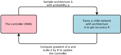Figure 1: An overview of Neural Architecture Search. <details> <summary>Image 1 Details</summary>  ### Visual Description \n ## Diagram: Neural Architecture Search Process ### Overview The image depicts a diagram illustrating a process for neural architecture search. It shows a cyclical flow between a controller (RNN) and a child network, with feedback used to update the controller. The diagram outlines a reinforcement learning approach to designing neural network architectures. ### Components/Axes The diagram consists of two main rectangular blocks connected by directed arrows, representing a feedback loop. Text labels are associated with each block and the arrows, describing the actions performed in each step. * **Block 1 (Pink):** "The controller (RNN)" * **Block 2 (Blue):** "Trains a child network with architecture A to get accuracy R" * **Arrow 1 (Top):** "Sample architecture A with probability p" * **Arrow 2 (Bottom):** "Compute gradient of p and scale it by R to update the controller" ### Detailed Analysis or Content Details The diagram illustrates a closed-loop process: 1. The controller, which is a Recurrent Neural Network (RNN), samples a neural network architecture (A) with a certain probability (p). 2. The sampled architecture (A) is used to train a child network. 3. The child network's performance is evaluated, resulting in an accuracy score (R). 4. The gradient of the probability (p) is computed and scaled by the accuracy (R). 5. This scaled gradient is then used to update the controller (RNN). 6. The process repeats, iteratively refining the controller's ability to sample effective architectures. ### Key Observations The diagram highlights a reinforcement learning paradigm where the controller learns to generate architectures that yield high accuracy. The accuracy (R) serves as a reward signal, guiding the controller's learning process. The use of gradients suggests a differentiable approach to architecture search. ### Interpretation This diagram represents a method for automating the design of neural network architectures. Instead of manually designing architectures, the controller learns to explore the architecture space and identify promising configurations. The feedback loop, driven by the accuracy of the child networks, allows the controller to adapt and improve its architecture sampling strategy over time. This approach can potentially discover architectures that outperform manually designed ones, especially for complex tasks. The diagram suggests a computationally intensive process, as it involves training multiple child networks. The use of an RNN as the controller implies that the architecture search process can leverage sequential dependencies and potentially discover architectures with complex structures. The scaling of the gradient by the accuracy (R) indicates that architectures with higher accuracy have a greater influence on updating the controller, effectively prioritizing the exploration of promising architecture regions. </details> This paper presents Neural Architecture Search, a gradient-based method for finding good architectures (see Figure 1) . Our work is based on the observation that the structure and connectivity of a ∗ Work done as a member of the Google Brain Residency program ( g.co/brainresidency .) neural network can be typically specified by a variable-length string. It is therefore possible to use a recurrent network - the controller - to generate such string. Training the network specified by the string - the 'child network' - on the real data will result in an accuracy on a validation set. Using this accuracy as the reward signal, we can compute the policy gradient to update the controller. As a result, in the next iteration, the controller will give higher probabilities to architectures that receive high accuracies. In other words, the controller will learn to improve its search over time. Our experiments show that Neural Architecture Search can design good models from scratch, an achievement considered not possible with other methods. On image recognition with CIFAR-10, Neural Architecture Search can find a novel ConvNet model that is better than most human-invented architectures. Our CIFAR-10 model achieves a 3.65 test set error, while being 1.05x faster than the current best model. On language modeling with Penn Treebank, Neural Architecture Search can design a novel recurrent cell that is also better than previous RNN and LSTM architectures. The cell that our model found achieves a test set perplexity of 62.4 on the Penn Treebank dataset, which is 3.6 perplexity better than the previous state-of-the-art. ## 2 RELATED WORK Hyperparameter optimization is an important research topic in machine learning, and is widely used in practice (Bergstra et al., 2011; Bergstra & Bengio, 2012; Snoek et al., 2012; 2015; Saxena & Verbeek, 2016). Despite their success, these methods are still limited in that they only search models from a fixed-length space. In other words, it is difficult to ask them to generate a variable-length configuration that specifies the structure and connectivity of a network. In practice, these methods often work better if they are supplied with a good initial model (Bergstra & Bengio, 2012; Snoek et al., 2012; 2015). There are Bayesian optimization methods that allow to search non fixed length architectures (Bergstra et al., 2013; Mendoza et al., 2016), but they are less general and less flexible than the method proposed in this paper. Modern neuro-evolution algorithms, e.g., Wierstra et al. (2005); Floreano et al. (2008); Stanley et al. (2009), on the other hand, are much more flexible for composing novel models, yet they are usually less practical at a large scale. Their limitations lie in the fact that they are search-based methods, thus they are slow or require many heuristics to work well. Neural Architecture Search has some parallels to program synthesis and inductive programming, the idea of searching a program from examples (Summers, 1977; Biermann, 1978). In machine learning, probabilistic program induction has been used successfully in many settings, such as learning to solve simple Q&A (Liang et al., 2010; Neelakantan et al., 2015; Andreas et al., 2016), sort a list of numbers (Reed & de Freitas, 2015), and learning with very few examples (Lake et al., 2015). The controller in Neural Architecture Search is auto-regressive, which means it predicts hyperparameters one a time, conditioned on previous predictions. This idea is borrowed from the decoder in end-to-end sequence to sequence learning (Sutskever et al., 2014). Unlike sequence to sequence learning, our method optimizes a non-differentiable metric, which is the accuracy of the child network. It is therefore similar to the work on BLEU optimization in Neural Machine Translation (Ranzato et al., 2015; Shen et al., 2016). Unlike these approaches, our method learns directly from the reward signal without any supervised bootstrapping. Also related to our work is the idea of learning to learn or meta-learning (Thrun & Pratt, 2012), a general framework of using information learned in one task to improve a future task. More closely related is the idea of using a neural network to learn the gradient descent updates for another network (Andrychowicz et al., 2016) and the idea of using reinforcement learning to find update policies for another network (Li & Malik, 2016). ## 3 METHODS In the following section, we will first describe a simple method of using a recurrent network to generate convolutional architectures. We will show how the recurrent network can be trained with a policy gradient method to maximize the expected accuracy of the sampled architectures. We will present several improvements of our core approach such as forming skip connections to increase model complexity and using a parameter server approach to speed up training. In the last part of the section, we will focus on generating recurrent architectures, which is another key contribution of our paper. 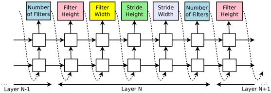## 3.1 GENERATE MODEL DESCRIPTIONS WITH A CONTROLLER RECURRENT NEURAL NETWORK In Neural Architecture Search, we use a controller to generate architectural hyperparameters of neural networks. To be flexible, the controller is implemented as a recurrent neural network. Let's suppose we would like to predict feedforward neural networks with only convolutional layers, we can use the controller to generate their hyperparameters as a sequence of tokens: Figure 2: How our controller recurrent neural network samples a simple convolutional network. It predicts filter height, filter width, stride height, stride width, and number of filters for one layer and repeats. Every prediction is carried out by a softmax classifier and then fed into the next time step as input. <details> <summary>Image 2 Details</summary>  ### Visual Description \n ## Diagram: Convolutional Neural Network Layer Configuration ### Overview The image depicts a diagram illustrating the configuration of layers in a convolutional neural network (CNN). It shows the connections between layers N-1, N, and N+1, highlighting key parameters associated with each layer. The diagram uses boxes to represent layers and arrows to indicate data flow and parameter influence. ### Components/Axes The diagram consists of the following components: * **Layers:** Represented as rectangular blocks, labeled "Layer N-1", "Layer N", and "Layer N+1" along the horizontal axis. * **Parameters:** Boxes positioned above the layers, labeled with: * "Number of Filters" (Light Blue) * "Filter Height" (Pink) * "Filter Width" (Yellow) * "Stride Height" (Light Green) * "Stride Width" (Dark Green) * **Data Flow:** Represented by solid arrows indicating the primary data path through the layers. * **Parameter Influence:** Represented by dashed arrows connecting the parameter boxes to the layers they influence. * **Horizontal Axis:** Indicates the progression of layers, labeled "...Layer N-1", "Layer N", "...Layer N+1". ### Detailed Analysis or Content Details The diagram illustrates how parameters from the parameter boxes influence the layers. Each layer receives input from the previous layer and passes output to the next. The parameters associated with each layer are: * **Layer N-1:** Influenced by "Number of Filters", "Filter Height", and "Filter Width". * **Layer N:** Influenced by "Filter Width", "Stride Height", and "Stride Width". * **Layer N+1:** Influenced by "Number of Filters", "Filter Height", and "Filter Width". The diagram does not provide specific numerical values for any of the parameters. It only shows the relationships between the layers and the parameters that affect them. The arrows indicate that the parameters influence the layers they point to. The solid arrows show the flow of data between layers. ### Key Observations * The diagram emphasizes the importance of parameters like filter size, stride, and the number of filters in defining the behavior of convolutional layers. * The parameters are not consistent across layers. For example, "Stride Height" and "Stride Width" only influence Layer N, while "Number of Filters" influences both Layer N-1 and Layer N+1. * The diagram is a conceptual representation and does not include details like padding, activation functions, or pooling layers. ### Interpretation This diagram illustrates the core concepts of convolutional layers in a CNN. It demonstrates how the choice of parameters (number of filters, filter size, stride) impacts the processing of data as it moves through the network. The diagram suggests that different layers may have different parameter configurations, allowing the network to learn hierarchical features. The use of dashed lines to represent parameter influence highlights that these parameters are not directly part of the data flow but rather control how the data is transformed. The diagram is a simplified representation, focusing on the key parameters and their relationships, and omitting other important aspects of CNN architecture. It serves as a visual aid for understanding the fundamental building blocks of a CNN. </details> In our experiments, the process of generating an architecture stops if the number of layers exceeds a certain value. This value follows a schedule where we increase it as training progresses. Once the controller RNN finishes generating an architecture, a neural network with this architecture is built and trained. At convergence, the accuracy of the network on a held-out validation set is recorded. The parameters of the controller RNN, θ c , are then optimized in order to maximize the expected validation accuracy of the proposed architectures. In the next section, we will describe a policy gradient method which we use to update parameters θ c so that the controller RNN generates better architectures over time. ## 3.2 TRAINING WITH REINFORCE The list of tokens that the controller predicts can be viewed as a list of actions a 1: T to design an architecture for a child network. At convergence, this child network will achieve an accuracy R on a held-out dataset. We can use this accuracy R as the reward signal and use reinforcement learning to train the controller. More concretely, to find the optimal architecture, we ask our controller to maximize its expected reward, represented by J ( θ c ) : $$J ( \theta _ { c } ) = E _ { P ( a _ { 1 \colon T } ; \theta _ { c } ) } [ R ]$$ Since the reward signal R is non-differentiable, we need to use a policy gradient method to iteratively update θ c . In this work, we use the REINFORCE rule from Williams (1992): $$\bigtriangledown _ { \theta _ { c } } J ( \theta _ { c } ) = \sum _ { t = 1 } ^ { T } E _ { P ( a _ { 1 \colon T } ; \theta _ { c } ) } \left [ \bigtriangledown _ { \theta _ { c } } \log P ( a _ { t } | a _ { ( t - 1 ) \colon 1 } ; \theta _ { c } ) R \right ]$$ An empirical approximation of the above quantity is: $$\frac { 1 } { m } \sum _ { k = 1 } ^ { m } \sum _ { t = 1 } ^ { T } \bigtriangledown _ { \theta _ { c } } \log P ( a _ { t } | a _ { ( t - 1 ) \colon 1 } ; \theta _ { c } ) R _ { k }$$ Where m is the number of different architectures that the controller samples in one batch and T is the number of hyperparameters our controller has to predict to design a neural network architecture. The validation accuracy that the k -th neural network architecture achieves after being trained on a training dataset is R k . The above update is an unbiased estimate for our gradient, but has a very high variance. In order to reduce the variance of this estimate we employ a baseline function: $$\frac { 1 } { m } \sum _ { k = 1 } ^ { m } \sum _ { t = 1 } ^ { T } \bigtriangledown _ { \theta _ { c } } \log P ( a _ { t } | a _ { ( t - 1 ) \colon 1 } ; \theta _ { c } ) ( R _ { k } - b )$$ As long as the baseline function b does not depend on the on the current action, then this is still an unbiased gradient estimate. In this work, our baseline b is an exponential moving average of the previous architecture accuracies. 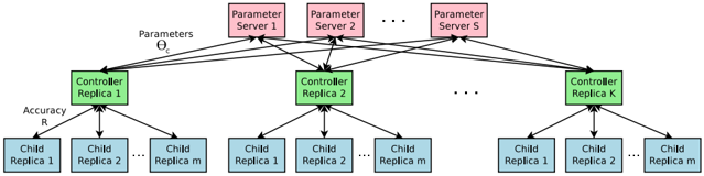Accelerate Training with Parallelism and Asynchronous Updates: In Neural Architecture Search, each gradient update to the controller parameters θ c corresponds to training one child network to convergence. As training a child network can take hours, we use distributed training and asynchronous parameter updates in order to speed up the learning process of the controller (Dean et al., 2012). We use a parameter-server scheme where we have a parameter server of S shards, that store the shared parameters for K controller replicas. Each controller replica samples m different child architectures that are trained in parallel. The controller then collects gradients according to the results of that minibatch of m architectures at convergence and sends them to the parameter server in order to update the weights across all controller replicas. In our implementation, convergence of each child network is reached when its training exceeds a certain number of epochs. This scheme of parallelism is summarized in Figure 3. Figure 3: Distributed training for Neural Architecture Search. We use a set of S parameter servers to store and send parameters to K controller replicas. Each controller replica then samples m architectures and run the multiple child models in parallel. The accuracy of each child model is recorded to compute the gradients with respect to θ c , which are then sent back to the parameter servers. <details> <summary>Image 3 Details</summary>  ### Visual Description \n ## Diagram: Federated Learning System Architecture ### Overview The image depicts a diagram of a federated learning system architecture. It illustrates the flow of parameters and accuracy information between parameter servers, controllers, and child replicas. The system appears to be designed for distributed machine learning, where models are trained across multiple devices without centralizing the training data. ### Components/Axes The diagram consists of three main types of components: * **Parameter Servers:** Labeled "Parameter Server 1", "Parameter Server 2", up to "Parameter Server S". These servers store and distribute model parameters. * **Controllers:** Labeled "Controller Replica 1", "Controller Replica 2", up to "Controller Replica K". These controllers manage the training process and coordinate with the child replicas. * **Child Replicas:** Labeled "Child Replica 1", "Child Replica 2", up to "Child Replica m". These replicas perform the actual model training on local data. There are two labeled arrows: * "Parameters Θ" pointing from the Parameter Servers to the Controllers. * "Accuracy R" pointing from the Controllers to the Child Replicas. ### Detailed Analysis / Content Details The diagram shows a multi-layered structure: 1. **Parameter Servers Layer (Top):** There are 'S' parameter servers. Each server holds model parameters. 2. **Controller Layer (Middle):** There are 'K' controller replicas. Each controller receives parameters from all 'S' parameter servers. 3. **Child Replica Layer (Bottom):** Each controller manages 'm' child replicas. Each child replica receives accuracy information from its respective controller. The connections between the layers are as follows: * Each parameter server sends parameters (Θ) to every controller replica. This indicates a broadcast mechanism. * Each controller replica sends accuracy information (R) to all of its child replicas. * The diagram does not show any connections *from* the child replicas to the controllers or parameter servers, suggesting that updates are not directly sent back, but rather aggregated and communicated through the controllers. The number of parameter servers is 'S', the number of controller replicas is 'K', and the number of child replicas per controller is 'm'. These are variables representing the scale of the system. ### Key Observations * The architecture is highly distributed. * The parameter servers act as a central repository for model parameters, but the controllers manage the training process. * The child replicas perform the local training and provide accuracy feedback to the controllers. * The diagram does not specify how the parameters are updated or how the accuracy information is used. * The use of "Replica" in the labels suggests redundancy and fault tolerance. ### Interpretation This diagram illustrates a federated learning setup. The parameter servers maintain the global model parameters, while the controllers orchestrate the training process across multiple child replicas. The child replicas train the model on their local data and report accuracy back to the controllers. This allows for distributed model training without sharing the raw data, preserving privacy. The architecture suggests a synchronous or semi-synchronous training process, where the controllers wait for feedback from all child replicas before updating the global model parameters. The broadcast of parameters from the servers to all controllers implies a desire for consistency across the replicas. The variables 'S', 'K', and 'm' allow for scaling the system to handle large datasets and complex models. The lack of direct connections from child replicas to parameter servers suggests that the controllers aggregate the updates before sending them to the parameter servers, potentially to reduce communication overhead or to implement privacy-preserving mechanisms like differential privacy. The diagram is a high-level overview and does not provide details about the specific algorithms or protocols used for parameter updates or accuracy aggregation. It focuses on the overall system architecture and the flow of information between the different components. 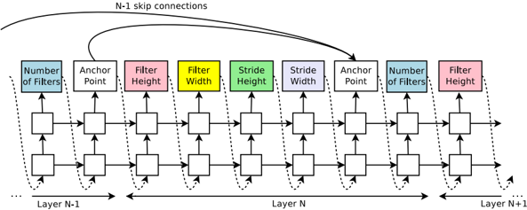</details> ## 3.3 INCREASE ARCHITECTURE COMPLEXITY WITH SKIP CONNECTIONS AND OTHER LAYER TYPES In Section 3.1, the search space does not have skip connections, or branching layers used in modern architectures such as GoogleNet (Szegedy et al., 2015), and Residual Net (He et al., 2016a). In this section we introduce a method that allows our controller to propose skip connections or branching layers, thereby widening the search space. To enable the controller to predict such connections, we use a set-selection type attention (Neelakantan et al., 2015) which was built upon the attention mechanism (Bahdanau et al., 2015; Vinyals et al., 2015). At layer N , we add an anchor point which has N -1 content-based sigmoids to indicate the previous layers that need to be connected. Each sigmoid is a function of the current hiddenstate of the controller and the previous hiddenstates of the previous N -1 anchor points: $$P ( L a y e r \, j \, i s \, a n \, i n p u t \, t o l a y e r \, i ) = s i g m o i d ( v ^ { T } \tanh ( W _ { p r e v } * h _ { j } + W _ { c u r r } * h _ { i } ) ) ,$$ where h j represents the hiddenstate of the controller at anchor point for the j -th layer, where j ranges from 0 to N -1 . We then sample from these sigmoids to decide what previous layers to be used as inputs to the current layer. The matrices W prev , W curr and v are trainable parameters. As these connections are also defined by probability distributions, the REINFORCE method still applies without any significant modifications. Figure 4 shows how the controller uses skip connections to decide what layers it wants as inputs to the current layer. Figure 4: The controller uses anchor points, and set-selection attention to form skip connections. <details> <summary>Image 4 Details</summary>  ### Visual Description \n ## Diagram: Neural Network Layer Architecture ### Overview The image depicts a diagram illustrating the architecture of consecutive layers (N-1, N, and N+1) in a neural network, likely a convolutional neural network (CNN). It highlights the flow of information and the parameters associated with each layer, including the number of filters, anchor point, filter height, filter width, and stride. Skip connections are also shown. ### Components/Axes The diagram consists of three main sections representing Layer N-1, Layer N, and Layer N+1, arranged horizontally. Each layer contains several blocks representing different parameters. The parameters are: * **Number of Filters:** Represented by light blue blocks. * **Anchor Point:** Represented by green blocks. * **Filter Height:** Represented by grey blocks, with one in red for Layer N+1. * **Filter Width:** Represented by yellow blocks. * **Stride Height:** Represented by teal blocks. * **Stride Width:** Represented by purple blocks. Dotted arrows indicate the flow of data between blocks within each layer. Curved arrows labeled "N-1 skip connections" show connections between Layer N-1 and Layer N+1. The horizontal axis represents the progression through layers. ### Detailed Analysis or Content Details The diagram shows a consistent structure across the three layers. Each layer receives input from the previous layer and passes output to the next. The parameters within each layer appear to be processed sequentially. * **Layer N-1:** The leftmost layer shows the flow of data through the parameters. * **Layer N:** The central layer shows the flow of data through the parameters. * **Layer N+1:** The rightmost layer shows the flow of data through the parameters. The "Filter Height" block is colored red, potentially indicating a specific or highlighted parameter. The skip connections bypass Layer N, directly connecting Layer N-1 to Layer N+1. This suggests a residual connection, a common technique in deep learning to mitigate the vanishing gradient problem. The diagram does not provide specific numerical values for any of the parameters. It only illustrates the conceptual flow and the types of parameters involved. ### Key Observations * The diagram emphasizes the modularity of neural network layers. * The skip connections suggest a residual network architecture. * The consistent structure across layers indicates a repeating pattern of processing. * The red "Filter Height" block in Layer N+1 might signify a specific configuration or a point of interest. ### Interpretation This diagram illustrates a common architectural pattern in deep convolutional neural networks. The parameters (number of filters, anchor point, filter height/width, stride) define the convolutional operations performed in each layer. The skip connections are a key feature of residual networks, allowing gradients to flow more easily through the network and enabling the training of deeper models. The diagram is a high-level representation and does not provide specific details about the network's functionality or performance. It serves as a visual aid for understanding the overall structure and data flow within the network. The diagram is a conceptual illustration, and does not contain any factual data. It is a schematic representation of a neural network architecture. </details> In our framework, if one layer has many input layers then all input layers are concatenated in the depth dimension. Skip connections can cause 'compilation failures' where one layer is not compatible with another layer, or one layer may not have any input or output. To circumvent these issues, we employ three simple techniques. First, if a layer is not connected to any input layer then the image is used as the input layer. Second, at the final layer we take all layer outputs that have not been connected and concatenate them before sending this final hiddenstate to the classifier. Lastly, if input layers to be concatenated have different sizes, we pad the small layers with zeros so that the concatenated layers have the same sizes. Finally, in Section 3.1, we do not predict the learning rate and we also assume that the architectures consist of only convolutional layers, which is also quite restrictive. It is possible to add the learning rate as one of the predictions. Additionally, it is also possible to predict pooling, local contrast normalization (Jarrett et al., 2009; Krizhevsky et al., 2012), and batchnorm (Ioffe & Szegedy, 2015) in the architectures. To be able to add more types of layers, we need to add an additional step in the controller RNN to predict the layer type, then other hyperparameters associated with it. ## 3.4 GENERATE RECURRENT CELL ARCHITECTURES In this section, we will modify the above method to generate recurrent cells. At every time step t , the controller needs to find a functional form for h t that takes x t and h t -1 as inputs. The simplest way is to have h t = tanh( W 1 ∗ x t + W 2 ∗ h t -1 ) , which is the formulation of a basic recurrent cell. A more complicated formulation is the widely-used LSTM recurrent cell (Hochreiter & Schmidhuber, 1997). The computations for basic RNN and LSTM cells can be generalized as a tree of steps that take x t and h t -1 as inputs and produce h t as final output. The controller RNN needs to label each node in the tree with a combination method (addition, elementwise multiplication, etc.) and an activation function ( tanh , sigmoid , etc.) to merge two inputs and produce one output. Two outputs are then fed as inputs to the next node in the tree. To allow the controller RNN to select these methods and functions, we index the nodes in the tree in an order so that the controller RNN can visit each node one by one and label the needed hyperparameters. Inspired by the construction of the LSTM cell (Hochreiter & Schmidhuber, 1997), we also need cell variables c t -1 and c t to represent the memory states. To incorporate these variables, we need the controller RNN to predict what nodes in the tree to connect these two variables to. These predictions can be done in the last two blocks of the controller RNN. 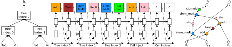To make this process more clear, we show an example in Figure 5, for a tree structure that has two leaf nodes and one internal node. The leaf nodes are indexed by 0 and 1, and the internal node is indexed by 2. The controller RNN needs to first predict 3 blocks, each block specifying a combination method and an activation function for each tree index. After that it needs to predict the last 2 blocks that specify how to connect c t and c t -1 to temporary variables inside the tree. Specifically, Figure 5: An example of a recurrent cell constructed from a tree that has two leaf nodes (base 2) and one internal node. Left: the tree that defines the computation steps to be predicted by controller. Center: an example set of predictions made by the controller for each computation step in the tree. Right: the computation graph of the recurrent cell constructed from example predictions of the controller. <details> <summary>Image 5 Details</summary>  ### Visual Description \n ## Diagram: LSTM Cell Structure ### Overview The image depicts the internal structure of a Long Short-Term Memory (LSTM) cell, a type of recurrent neural network (RNN) architecture. It shows the flow of information through various gates and operations within the cell. The diagram is split into three main sections: a tree-like representation of cell indices, a horizontal sequence of operations, and a zoomed-in view of a portion of the cell. ### Components/Axes The diagram contains the following components: * **Input:** `xₜ` (input at time t) and `hₜ₋₁` (hidden state at time t-1). * **Gates/Operations:** Add, Tanh, Element-wise Multiplication (Elem Mult), ReLU, Sigmoid, Cell Inject. * **Cell State:** Represented by horizontal lines flowing through the operations. * **Output:** `hₜ` (hidden state at time t). * **Tree Indices:** Tree Index 0, Tree Index 1, Tree Index 2. * **Cell Indices:** Cell Inject, Cell Indices. * **Labels:** Add, Tanh, Elem Mult, ReLU, Sigmoid, Add, 1, 0, sigmoid, relu, elem_mult, add, tanh. ### Detailed Analysis or Content Details **Left Section (Tree Indices):** This section shows a binary tree structure. * The root node is labeled "Tree Index 2". * It branches into "Tree Index 0" and "Tree Index 1". * "Tree Index 0" receives inputs from `hₜ₋₁` and `xₜ`. * "Tree Index 1" receives inputs from `hₜ₋₁` and `xₜ`. * The output of the tree structure feeds into the main LSTM cell operations. **Middle Section (LSTM Cell Operations):** This section shows a sequence of operations applied to the cell state. The operations are arranged horizontally. 1. **Add:** Receives input from Tree Index 0 and the cell state. Output is colored red. 2. **Tanh:** Receives input from the previous Add operation. Output is colored red. 3. **Elem Mult:** Receives input from Tree Index 1 and the previous Tanh operation. Output is colored blue. 4. **ReLU:** Receives input from the previous Elem Mult operation. Output is colored blue. 5. **Elem Mult:** Receives input from Tree Index 2 and the previous ReLU operation. Output is colored green. 6. **Sigmoid:** Receives input from the previous Elem Mult operation. Output is colored green. 7. **Add:** Receives input from the previous Sigmoid operation and the cell state. Output is colored orange. 8. **1:** A constant value of 1. 9. **0:** A constant value of 0. **Right Section (Zoomed-in View):** This section provides a more detailed view of a portion of the LSTM cell. * `xₜ` and `hₜ₋₁` are inputs. * The operations shown are: elem_mult, relu, add, tanh, add, sigmoid. * The output is `hₜ`. ### Key Observations * The LSTM cell utilizes multiple gates (Tanh, Sigmoid) and element-wise multiplications to control the flow of information. * The tree structure on the left appears to represent a hierarchical decomposition of the cell state updates. * The ReLU activation function is used to introduce non-linearity. * The constant values 1 and 0 likely represent gating mechanisms. ### Interpretation The diagram illustrates the complex internal workings of an LSTM cell. The tree structure suggests a way to organize and process information within the cell, potentially allowing for more efficient learning of long-term dependencies. The various gates and operations work together to regulate the flow of information, enabling the LSTM cell to selectively remember or forget information from previous time steps. The use of element-wise multiplication and non-linear activation functions (Tanh, ReLU, Sigmoid) allows the cell to learn complex patterns in the input data. The diagram highlights the key components and their interactions, providing a visual representation of the LSTM cell's functionality. The zoomed-in view emphasizes the specific operations involved in updating the hidden state. The diagram is a simplified representation of the LSTM cell, focusing on the core computational steps. It does not show the weight matrices or biases associated with each operation. </details> according to the predictions of the controller RNN in this example, the following computation steps will occur: - The controller predicts Add and Tanh for tree index 0, this means we need to compute a 0 = tanh( W 1 ∗ x t + W 2 ∗ h t -1 ) . - The controller predicts ElemMult and ReLU for tree index 1, this means we need to compute a 1 = ReLU ( ( W 3 ∗ x t ) ( W 4 ∗ h t -1 ) ) . - The controller predicts 0 for the second element of the 'Cell Index', Add and ReLU for elements in 'Cell Inject', which means we need to compute a new 0 = ReLU( a 0 + c t -1 ) . Notice that we don't have any learnable parameters for the internal nodes of the tree. - The controller predicts ElemMult and Sigmoid for tree index 2, this means we need to compute a 2 = sigmoid( a new 0 a 1 ) . Since the maximum index in the tree is 2, h t is set to a 2 . - The controller RNN predicts 1 for the first element of the 'Cell Index', this means that we should set c t to the output of the tree at index 1 before the activation, i.e., c t = ( W 3 ∗ x t ) ( W 4 ∗ h t -1 ) . In the above example, the tree has two leaf nodes, thus it is called a 'base 2' architecture. In our experiments, we use a base number of 8 to make sure that the cell is expressive. ## 4 EXPERIMENTS AND RESULTS We apply our method to an image classification task with CIFAR-10 and a language modeling task with Penn Treebank, two of the most benchmarked datasets in deep learning. On CIFAR-10, our goal is to find a good convolutional architecture whereas on Penn Treebank our goal is to find a good recurrent cell. On each dataset, we have a separate held-out validation dataset to compute the reward signal. The reported performance on the test set is computed only once for the network that achieves the best result on the held-out validation dataset. More details about our experimental procedures and results are as follows. ## 4.1 LEARNING CONVOLUTIONAL ARCHITECTURES FOR CIFAR-10 Dataset: In these experiments we use the CIFAR-10 dataset with data preprocessing and augmentation procedures that are in line with other previous results. We first preprocess the data by whitening all the images. Additionally, we upsample each image then choose a random 32x32 crop of this upsampled image. Finally, we use random horizontal flips on this 32x32 cropped image. Search space: Our search space consists of convolutional architectures, with rectified linear units as non-linearities (Nair & Hinton, 2010), batch normalization (Ioffe & Szegedy, 2015) and skip connections between layers (Section 3.3). For every convolutional layer, the controller RNN has to select a filter height in [1, 3, 5, 7], a filter width in [1, 3, 5, 7], and a number of filters in [24, 36, 48, 64]. For strides, we perform two sets of experiments, one where we fix the strides to be 1, and one where we allow the controller to predict the strides in [1, 2, 3]. Training details: The controller RNN is a two-layer LSTM with 35 hidden units on each layer. It is trained with the ADAM optimizer (Kingma & Ba, 2015) with a learning rate of 0.0006. The weights of the controller are initialized uniformly between -0.08 and 0.08. For the distributed training, we set the number of parameter server shards S to 20, the number of controller replicas K to 100 and the number of child replicas m to 8, which means there are 800 networks being trained on 800 GPUs concurrently at any time. Once the controller RNN samples an architecture, a child model is constructed and trained for 50 epochs. The reward used for updating the controller is the maximum validation accuracy of the last 5 epochs cubed. The validation set has 5,000 examples randomly sampled from the training set, the remaining 45,000 examples are used for training. The settings for training the CIFAR-10 child models are the same with those used in Huang et al. (2016a). We use the Momentum Optimizer with a learning rate of 0.1, weight decay of 1e-4, momentum of 0.9 and used Nesterov Momentum (Sutskever et al., 2013). During the training of the controller, we use a schedule of increasing number of layers in the child networks as training progresses. On CIFAR-10, we ask the controller to increase the depth by 2 for the child models every 1,600 samples, starting at 6 layers. Results: After the controller trains 12,800 architectures, we find the architecture that achieves the best validation accuracy. We then run a small grid search over learning rate, weight decay, batchnorm epsilon and what epoch to decay the learning rate. The best model from this grid search is then run until convergence and we then compute the test accuracy of such model and summarize the results in Table 1. As can be seen from the table, Neural Architecture Search can design several promising architectures that perform as well as some of the best models on this dataset. | Model | Depth | Parameters | Error rate (%) | |-----------------------------------------------------|----------|--------------|------------------| | Network in Network (Lin et al., 2013) | - | - | 8.81 | | All-CNN (Springenberg et al., 2014) | - | - | 7.25 | | Deeply Supervised Net (Lee et al., 2015) | - | - | 7.97 | | Highway Network (Srivastava et al., 2015) | - | - | 7.72 | | Scalable Bayesian Optimization (Snoek et al., 2015) | - | - | 6.37 | | FractalNet (Larsson et al., 2016) | 21 | 38.6M | 5.22 | | with Dropout/Drop-path | 21 | 38.6M | 4.60 | | ResNet (He et al., 2016a) | 110 | 1.7M | 6.61 | | ResNet (reported by Huang et al. (2016c)) | 110 | 1.7M | 6.41 | | ResNet with Stochastic Depth (Huang et al., 2016c) | 110 | 1.7M | 5.23 | | Wide ResNet (Zagoruyko &Komodakis, 2016) | 16 | 11.0M | 4.81 | | | 28 | 36.5M | 4.17 | | ResNet (pre-activation) (He et al., 2016b) | 164 1001 | 1.7M 10.2M | 5.46 | | DenseNet ( L = 40 ,k = 12) Huang et al. (2016a) | | 1.0M | 4.62 5.24 | | | 40 | | | | DenseNet ( L = 100 ,k = 12) Huang et al. (2016a) | 100 | 7.0M | 4.10 | | DenseNet ( L = 100 ,k = 24) Huang et al. (2016a) | 100 | 27.2M | 3.74 | | DenseNet-BC ( L = 100 ,k = 40) Huang et al. (2016b) | 190 | 25.6M | 3.46 | | Neural Architecture Search v1 no stride or pooling | 15 | 4.2M | 5.50 | | Neural Architecture Search v2 predicting strides | 20 | 2.5M | 6.01 | | Neural Architecture Search v3 max pooling | 39 | 7.1M | 4.47 | | Neural Architecture Search v3 max pooling + more | 39 | | 3.65 | | filters | | 37.4M | | Table 1: Performance of Neural Architecture Search and other state-of-the-art models on CIFAR-10. 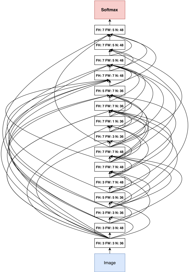First, if we ask the controller to not predict stride or pooling, it can design a 15-layer architecture that achieves 5.50% error rate on the test set. This architecture has a good balance between accuracy and depth. In fact, it is the shallowest and perhaps the most inexpensive architecture among the top performing networks in this table. This architecture is shown in Appendix A, Figure 7. A notable feature of this architecture is that it has many rectangular filters and it prefers larger filters at the top layers. Like residual networks (He et al., 2016a), the architecture also has many one-step skip connections. This architecture is a local optimum in the sense that if we perturb it, its performance becomes worse. For example, if we densely connect all layers with skip connections, its performance becomes slightly worse: 5.56%. If we remove all skip connections, its performance drops to 7.97%. In the second set of experiments, we ask the controller to predict strides in addition to other hyperparameters. As stated earlier, this is more challenging because the search space is larger. In this case, it finds a 20-layer architecture that achieves 6.01% error rate on the test set, which is not much worse than the first set of experiments. Finally, if we allow the controller to include 2 pooling layers at layer 13 and layer 24 of the architectures, the controller can design a 39-layer network that achieves 4.47% which is very close to the best human-invented architecture that achieves 3.74%. To limit the search space complexity we have our model predict 13 layers where each layer prediction is a fully connected block of 3 layers. Additionally, we change the number of filters our model can predict from [24, 36, 48, 64] to [6, 12, 24, 36]. Our result can be improved to 3.65% by adding 40 more filters to each layer of our architecture. Additionally this model with 40 filters added is 1.05x as fast as the DenseNet model that achieves 3.74%, while having better performance. The DenseNet model that achieves 3.46% error rate (Huang et al., 2016b) uses 1x1 convolutions to reduce its total number of parameters, which we did not do, so it is not an exact comparison. ## 4.2 LEARNING RECURRENT CELLS FOR PENN TREEBANK Dataset: Weapply Neural Architecture Search to the Penn Treebank dataset, a well-known benchmark for language modeling. On this task, LSTM architectures tend to excel (Zaremba et al., 2014; Gal, 2015), and improving them is difficult (Jozefowicz et al., 2015). As PTB is a small dataset, regularization methods are needed to avoid overfitting. First, we make use of the embedding dropout and recurrent dropout techniques proposed in Zaremba et al. (2014) and (Gal, 2015). We also try to combine them with the method of sharing Input and Output embeddings, e.g., Bengio et al. (2003); Mnih & Hinton (2007), especially Inan et al. (2016) and Press & Wolf (2016). Results with this method are marked with 'shared embeddings.' Search space: Following Section 3.4, our controller sequentially predicts a combination method then an activation function for each node in the tree. For each node in the tree, the controller RNN needs to select a combination method in [ add, elem mult ] and an activation method in [ identity, tanh, sigmoid, relu ] . The number of input pairs to the RNN cell is called the 'base number' and set to 8 in our experiments. When the base number is 8, the search space is has approximately 6 × 10 16 architectures, which is much larger than 15,000, the number of architectures that we allow our controller to evaluate. Training details: The controller and its training are almost identical to the CIFAR-10 experiments except for a few modifications: 1) the learning rate for the controller RNN is 0.0005, slightly smaller than that of the controller RNN in CIFAR-10, 2) in the distributed training, we set S to 20, K to 400 and m to 1, which means there are 400 networks being trained on 400 CPUs concurrently at any time, 3) during asynchronous training we only do parameter updates to the parameter-server once 10 gradients from replicas have been accumulated. In our experiments, every child model is constructed and trained for 35 epochs. Every child model has two layers, with the number of hidden units adjusted so that total number of learnable parameters approximately match the 'medium' baselines (Zaremba et al., 2014; Gal, 2015). In these experiments we only have the controller predict the RNN cell structure and fix all other hyperparameters. The reward function is c (validation perplexity) 2 where c is a constant, usually set at 80. After the controller RNN is done training, we take the best RNN cell according to the lowest validation perplexity and then run a grid search over learning rate, weight initialization, dropout rates and decay epoch. The best cell found was then run with three different configurations and sizes to increase its capacity. Results: In Table 2, we provide a comprehensive list of architectures and their performance on the PTB dataset. As can be seen from the table, the models found by Neural Architecture Search outperform other state-of-the-art models on this dataset, and one of our best models achieves a gain of almost 3.6 perplexity. Not only is our cell is better, the model that achieves 64 perplexity is also more than two times faster because the previous best network requires running a cell 10 times per time step (Zilly et al., 2016). Table 2: Single model perplexity on the test set of the Penn Treebank language modeling task. Parameter numbers with ‡ are estimates with reference to Merity et al. (2016). | Model | Parameters | Test Perplexity | |--------------------------------------------------------------|--------------|-------------------| | Mikolov &Zweig (2012) - KN-5 | 2M ‡ | 141 . 2 | | Mikolov &Zweig (2012) - KN5 + cache | 2M ‡ | 125 . 7 | | Mikolov &Zweig (2012) - RNN | 6M ‡ | 124 . 7 | | Mikolov &Zweig (2012) - RNN-LDA | 7M ‡ | 113 . 7 | | Mikolov &Zweig (2012) - RNN-LDA + KN-5 + cache | 9M ‡ | 92 . 0 | | Pascanu et al. (2013) - Deep RNN | 6M | 107 . 5 | | Cheng et al. (2014) - Sum-Prod Net | 5M ‡ | 100 . 0 | | Zaremba et al. (2014) - LSTM (medium) | 20M | 82 . 7 | | Zaremba et al. (2014) - LSTM (large) | 66M | 78 . 4 | | Gal (2015) - Variational LSTM (medium, untied) | 20M | 79 . 7 | | Gal (2015) - Variational LSTM (medium, untied, MC) | 20M | 78 . 6 | | Gal (2015) - Variational LSTM (large, untied) | 66M | 75 . 2 | | Gal (2015) - Variational LSTM (large, untied, MC) | 66M | 73 . 4 | | Kim et al. (2015) - CharCNN | 19M | 78 . 9 | | Press &Wolf (2016) - Variational LSTM, shared embeddings | 51M | 73 . 2 | | Merity et al. (2016) - Zoneout + Variational LSTM (medium) | 20M | 80 . 6 | | Merity et al. (2016) - Pointer Sentinel-LSTM (medium) | 21M | 70 . 9 | | Inan et al. (2016) - VD-LSTM + REAL (large) | 51M | 68 . 5 | | Zilly et al. (2016) - Variational RHN, shared embeddings | 24M | 66 . 0 | | Neural Architecture Search with base 8 | 32M | 67 . 9 | | Neural Architecture Search with base 8 and shared embeddings | 25M | 64 . 0 | | Neural Architecture Search with base 8 and shared embeddings | 54M | 62 . 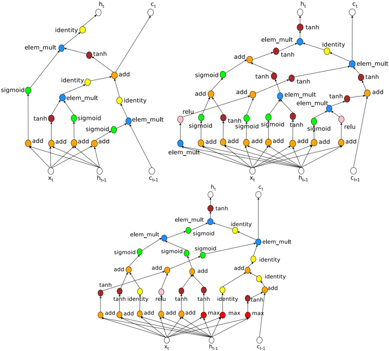4 | The newly discovered cell is visualized in Figure 8 in Appendix A. The visualization reveals that the new cell has many similarities to the LSTM cell in the first few steps, such as it likes to compute W 1 ∗ h t -1 + W 2 ∗ x t several times and send them to different components in the cell. Transfer Learning Results: To understand whether the cell can generalize to a different task, we apply it to the character language modeling task on the same dataset. We use an experimental setup that is similar to Ha et al. (2016), but use variational dropout by Gal (2015). We also train our own LSTM with our setup to get a fair LSTM baseline. Models are trained for 80K steps and the best test set perplexity is taken according to the step where validation set perplexity is the best. The results on the test set of our method and state-of-art methods are reported in Table 3. The results on small settings with 5-6M parameters confirm that the new cell does indeed generalize, and is better than the LSTM cell. Additionally, we carry out a larger experiment where the model has 16.28M parameters. This model has a weight decay rate of 1 e -4 , was trained for 600K steps (longer than the above models) and the test perplexity is taken where the validation set perplexity is highest. We use dropout rates of 0.2 and 0.5 as described in Gal (2015), but do not use embedding dropout. We use the ADAM optimizer with a learning rate of 0.001 and an input embedding size of 128. Our model had two layers with 800 hidden units. We used a minibatch size of 32 and BPTT length of 100. With this setting, our model achieves 1.214 perplexity, which is the new state-of-the-art result on this task. Finally, we also drop our cell into the GNMT framework (Wu et al., 2016), which was previously tuned for LSTM cells, and train an WMT14 English → German translation model. The GNMT Table 3: Comparison between our cell and state-of-art methods on PTB character modeling. The new cell was found on word level language modeling. | RNN Cell Type | Parameters | Test Bits Per Character | |----------------------------------------------------------|--------------|---------------------------| | Ha et al. (2016) - Layer Norm HyperLSTM | 4.92M | 1.25 | | Ha et al. (2016) - Layer Norm HyperLSTM Large Embeddings | 5.06M | 1.233 | | Ha et al. (2016) - 2-Layer Norm HyperLSTM | 14.41M | 1.219 | | Two layer LSTM | 6.57M | 1.243 | | Two Layer with New Cell | 6.57M | 1.228 | | Two Layer with New Cell | 16.28M | 1.214 | network has 8 layers in the encoder, 8 layers in the decoder. The first layer of the encoder has bidirectional connections. The attention module is a neural network with 1 hidden layer. When a LSTM cell is used, the number of hidden units in each layer is 1024. The model is trained in a distributed setting with a parameter sever and 12 workers. Additionally, each worker uses 8 GPUs and a minibatch of 128. We use Adam with a learning rate of 0.0002 in the first 60K training steps, and SGD with a learning rate of 0.5 until 400K steps. After that the learning rate is annealed by dividing by 2 after every 100K steps until it reaches 0.1. Training is stopped at 800K steps. More details can be found in Wu et al. (2016). In our experiment with the new cell, we make no change to the above settings except for dropping in the new cell and adjusting the hyperparameters so that the new model should have the same computational complexity with the base model. The result shows that our cell, with the same computational complexity, achieves an improvement of 0.5 test set BLEU than the default LSTM cell. Though this improvement is not huge, the fact that the new cell can be used without any tuning on the existing GNMT framework is encouraging. We expect further tuning can help our cell perform better. Control Experiment 1 - Adding more functions in the search space: To test the robustness of Neural Architecture Search, we add max to the list of combination functions and sin to the list of activation functions and rerun our experiments. The results show that even with a bigger search space, the model can achieve somewhat comparable performance. The best architecture with max and sin is shown in Figure 8 in Appendix A. 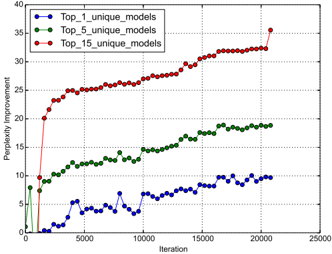Control Experiment 2 - Comparison against Random Search: Instead of policy gradient, one can use random search to find the best network. Although this baseline seems simple, it is often very hard to surpass (Bergstra & Bengio, 2012). We report the perplexity improvements using policy gradient against random search as training progresses in Figure 6. The results show that not only the best model using policy gradient is better than the best model using random search, but also the average of top models is also much better. Figure 6: Improvement of Neural Architecture Search over random search over time. We plot the difference between the average of the top k models our controller finds vs. random search every 400 models run. <details> <summary>Image 6 Details</summary>  ### Visual Description \n ## Line Chart: Perplexity Improvement vs. Iteration ### Overview The image presents a line chart illustrating the relationship between iteration number and perplexity improvement for three different model configurations: Top_1_unique_models, Top_5_unique_models, and Top_15_unique_models. The chart displays how perplexity improvement changes as the number of iterations increases. ### Components/Axes * **X-axis:** Iteration (ranging from approximately 0 to 25000) * **Y-axis:** Perplexity Improvement (ranging from approximately 0 to 40) * **Data Series:** * Top_1_unique_models (Blue line with circle markers) * Top_5_unique_models (Green line with triangle markers) * Top_15_unique_models (Red line with circle markers) * **Legend:** Located in the top-left corner, clearly labeling each data series with its corresponding color. ### Detailed Analysis * **Top_1_unique_models (Blue):** The line initially fluctuates around a perplexity improvement of approximately 2-8 for the first 5000 iterations. It then exhibits more pronounced oscillations, reaching a peak of around 12 at approximately 7500 iterations, before settling around 8-10 for the remainder of the iterations, ending at approximately 9 at 20000 iterations. * **Top_5_unique_models (Green):** This line shows a consistent upward trend from the beginning. Starting at approximately 10 at iteration 0, it steadily increases to around 15 at 5000 iterations, and continues to rise, reaching approximately 22 at 20000 iterations. The slope of this line is relatively constant throughout. * **Top_15_unique_models (Red):** This line demonstrates the most significant and rapid improvement. It starts at approximately 20 at iteration 0 and quickly rises to around 25 at 5000 iterations. The improvement continues at a slightly decreasing rate, reaching approximately 32 at 15000 iterations, and finally leveling off around 34 at 20000 iterations. There is a slight dip to approximately 31 at 22000 iterations. ### Key Observations * The Top_15_unique_models consistently exhibits the highest perplexity improvement throughout all iterations. * The Top_5_unique_models shows a steady, moderate improvement. * The Top_1_unique_models demonstrates the least improvement and the most fluctuation. * All three models show diminishing returns in perplexity improvement as the number of iterations increases. The rate of improvement slows down over time. * The initial jump in perplexity improvement for the Top_15_unique_models is particularly noticeable. ### Interpretation The chart suggests that increasing the number of unique models considered (from 1 to 5 to 15) leads to a higher overall perplexity improvement during the training process. This indicates that exploring a wider range of model configurations can result in better performance. The diminishing returns observed in all three models suggest that there is a point beyond which further iterations provide only marginal improvements. The fluctuations in the Top_1_unique_models line might indicate instability or sensitivity to the specific training data. The data demonstrates a clear trade-off between model complexity (number of unique models) and performance (perplexity improvement). The Top_15 model achieves the best performance, but it also likely requires more computational resources and training time. The chart provides valuable insights into the optimization process and can help guide decisions about model selection and training duration. </details> ## 5 CONCLUSION In this paper we introduce Neural Architecture Search, an idea of using a recurrent neural network to compose neural network architectures. By using recurrent network as the controller, our method is flexible so that it can search variable-length architecture space. Our method has strong empirical performance on very challenging benchmarks and presents a new research direction for automatically finding good neural network architectures. The code for running the models found by the controller on CIFAR-10 and PTB will be released at https://github.com/tensorflow/models . Additionally, we have added the RNN cell found using our method under the name NASCell into TensorFlow, so others can easily use it. ## ACKNOWLEDGMENTS We thank Greg Corrado, Jeff Dean, David Ha, Lukasz Kaiser and the Google Brain team for their help with the project. ## REFERENCES - Jacob Andreas, Marcus Rohrbach, Trevor Darrell, and Dan Klein. Learning to compose neural networks for question answering. In NAACL , 2016. - Marcin Andrychowicz, Misha Denil, Sergio Gomez, Matthew W Hoffman, David Pfau, Tom Schaul, and Nando de Freitas. Learning to learn by gradient descent by gradient descent. arXiv preprint arXiv:1606.04474 , 2016. - Dzmitry Bahdanau, Kyunghyun Cho, and Yoshua Bengio. Neural machine translation by jointly learning to align and translate. In ICLR , 2015. - Yoshua Bengio, R´ ejean Ducharme, Pascal Vincent, and Christian Jauvin. A neural probabilistic language model. JMLR , 2003. - James Bergstra and Yoshua Bengio. Random search for hyper-parameter optimization. JMLR , 2012. - James Bergstra, R´ emi Bardenet, Yoshua Bengio, and Bal´ azs K´ egl. Algorithms for hyper-parameter optimization. In NIPS , 2011. - James Bergstra, Daniel Yamins, and David D Cox. Making a science of model search: Hyperparameter optimization in hundreds of dimensions for vision architectures. ICML , 2013. - Alan W. Biermann. The inference of regular LISP programs from examples. IEEE transactions on Systems, Man, and Cybernetics , 1978. - Wei-Chen Cheng, Stanley Kok, Hoai Vu Pham, Hai Leong Chieu, and Kian Ming Adam Chai. Language modeling with sum-product networks. In INTERSPEECH , 2014. - Navneet Dalal and Bill Triggs. Histograms of oriented gradients for human detection. In CVPR , 2005. - Jeffrey Dean, Greg Corrado, Rajat Monga, Kai Chen, Matthieu Devin, Mark Mao, Andrew Senior, Paul Tucker, Ke Yang, Quoc V. Le, et al. Large scale distributed deep networks. In NIPS , 2012. - Dario Floreano, Peter D¨ urr, and Claudio Mattiussi. Neuroevolution: from architectures to learning. Evolutionary Intelligence , 2008. - Yarin Gal. A theoretically grounded application of dropout in recurrent neural networks. arXiv preprint arXiv:1512.05287 , 2015. - David Ha, Andrew Dai, and Quoc V. Le. Hypernetworks. arXiv preprint arXiv:1609.09106 , 2016. - Kaiming He, Xiangyu Zhang, Shaoqing Ren, and Jian Sun. Deep residual learning for image recognition. In CVPR , 2016a. - Kaiming He, Xiangyu Zhang, Shaoqing Ren, and Jian Sun. Identity mappings in deep residual networks. arXiv preprint arXiv:1603.05027 , 2016b. - Geoffrey Hinton, Li Deng, Dong Yu, George E. Dahl, Abdel-rahman Mohamed, Navdeep Jaitly, Andrew Senior, Vincent Vanhoucke, Patrick Nguyen, Tara N. Sainath, et al. Deep neural networks for acoustic modeling in speech recognition: The shared views of four research groups. IEEE Signal Processing Magazine , 2012. - Sepp Hochreiter and Juergen Schmidhuber. Long short-term memory. Neural Computation , 1997. - Gao Huang, Zhuang Liu, and Kilian Q. Weinberger. Densely connected convolutional networks. arXiv preprint arXiv:1608.06993 , 2016a. - Gao Huang, Zhuang Liu, Kilian Q. Weinberger, and Laurens van der Maaten. Densely connected convolutional networks. arXiv preprint arXiv:1608.06993 , 2016b. - Gao Huang, Yu Sun, Zhuang Liu, Daniel Sedra, and Kilian Weinberger. Deep networks with stochastic depth. arXiv preprint arXiv:1603.09382 , 2016c. - Hakan Inan, Khashayar Khosravi, and Richard Socher. Tying word vectors and word classifiers: A loss framework for language modeling. arXiv preprint arXiv:1611.01462 , 2016. - Sergey Ioffe and Christian Szegedy. Batch normalization: Accelerating deep network training by reducing internal covariate shift. In ICML , 2015. - Kevin Jarrett, Koray Kavukcuoglu, Yann Lecun, et al. What is the best multi-stage architecture for object recognition? In ICCV , 2009. - Rafal Jozefowicz, Wojciech Zaremba, and Ilya Sutskever. An empirical exploration of recurrent network architectures. In ICML , 2015. - Yoon Kim, Yacine Jernite, David Sontag, and Alexander M. Rush. Character-aware neural language models. arXiv preprint arXiv:1508.06615 , 2015. - Diederik P. Kingma and Jimmy Ba. Adam: A method for stochastic optimization. In ICLR , 2015. - Alex Krizhevsky, Ilya Sutskever, and Geoffrey E. Hinton. Imagenet classification with deep convolutional neural networks. In NIPS , 2012. - Brenden M. Lake, Ruslan Salakhutdinov, and Joshua B. Tenenbaum. Human-level concept learning through probabilistic program induction. Science , 2015. - Gustav Larsson, Michael Maire, and Gregory Shakhnarovich. Fractalnet: Ultra-deep neural networks without residuals. arXiv preprint arXiv:1605.07648 , 2016. - Yann LeCun, L´ eon Bottou, Yoshua Bengio, and Patrick Haffner. Gradient-based learning applied to document recognition. Proceedings of the IEEE , 1998. - Chen-Yu Lee, Saining Xie, Patrick Gallagher, Zhengyou Zhang, and Zhuowen Tu. Deeplysupervised nets. In AISTATS , 2015. - Ke Li and Jitendra Malik. Learning to optimize. arXiv preprint arXiv:1606.01885 , 2016. - Percy Liang, Michael I. Jordan, and Dan Klein. Learning programs: A hierarchical Bayesian approach. In ICML , 2010. - Min Lin, Qiang Chen, and Shuicheng Yan. Network in network. In ICLR , 2013. - David G. Lowe. Object recognition from local scale-invariant features. In CVPR , 1999. - Hector Mendoza, Aaron Klein, Matthias Feurer, Jost Tobias Springenberg, and Frank Hutter. Towards automatically-tuned neural networks. In Proceedings of the 2016 Workshop on Automatic Machine Learning , pp. 58-65, 2016. - Stephen Merity, Caiming Xiong, James Bradbury, and Richard Socher. Pointer sentinel mixture models. arXiv preprint arXiv:1609.07843 , 2016. - Tomas Mikolov and Geoffrey Zweig. Context dependent recurrent neural network language model. In SLT , pp. 234-239, 2012. - Andriy Mnih and Geoffrey Hinton. Three new graphical models for statistical language modelling. In ICML , 2007. - Vinod Nair and Geoffrey E. Hinton. Rectified linear units improve restricted Boltzmann machines. In ICML , 2010. - Arvind Neelakantan, Quoc V. Le, and Ilya Sutskever. Neural programmer: Inducing latent programs with gradient descent. In ICLR , 2015. - Razvan Pascanu, Caglar Gulcehre, Kyunghyun Cho, and Yoshua Bengio. How to construct deep recurrent neural networks. arXiv preprint arXiv:1312.6026 , 2013. - Ofir Press and Lior Wolf. Using the output embedding to improve language models. arXiv preprint arXiv:1608.05859 , 2016. - Marc'Aurelio Ranzato, Sumit Chopra, Michael Auli, and Wojciech Zaremba. Sequence level training with recurrent neural networks. arXiv preprint arXiv:1511.06732 , 2015. - Scott Reed and Nando de Freitas. Neural programmer-interpreters. In ICLR , 2015. - Shreyas Saxena and Jakob Verbeek. Convolutional neural fabrics. In NIPS , 2016. - Shiqi Shen, Yong Cheng, Zhongjun He, Wei He, Hua Wu, Maosong Sun, and Yang Liu. Minimum risk training for neural machine translation. In ACL , 2016. - Karen Simonyan and Andrew Zisserman. Very deep convolutional networks for large-scale image recognition. arXiv preprint arXiv:1409.1556 , 2014. - Jasper Snoek, Hugo Larochelle, and Ryan P. Adams. Practical Bayesian optimization of machine learning algorithms. In NIPS , 2012. - Jasper Snoek, Oren Rippel, Kevin Swersky, Ryan Kiros, Nadathur Satish, Narayanan Sundaram, Mostofa Patwary, Mostofa Ali, Ryan P. Adams, et al. Scalable bayesian optimization using deep neural networks. In ICML , 2015. - Jost Tobias Springenberg, Alexey Dosovitskiy, Thomas Brox, and Martin Riedmiller. Striving for simplicity: The all convolutional net. arXiv preprint arXiv:1412.6806 , 2014. - Rupesh Kumar Srivastava, Klaus Greff, and J¨ urgen Schmidhuber. Highway networks. arXiv preprint arXiv:1505.00387 , 2015. - Kenneth O. Stanley, David B. D'Ambrosio, and Jason Gauci. A hypercube-based encoding for evolving large-scale neural networks. Artificial Life , 2009. - Phillip D. Summers. A methodology for LISP program construction from examples. Journal of the ACM , 1977. - Ilya Sutskever, James Martens, George Dahl, and Geoffrey Hinton. On the importance of initialization and momentum in deep learning. In ICML , 2013. - Ilya Sutskever, Oriol Vinyals, and Quoc V. Le. Sequence to sequence learning with neural networks. In NIPS , 2014. - Christian Szegedy, Wei Liu, Yangqing Jia, Pierre Sermanet, Scott Reed, Dragomir Anguelov, Dumitru Erhan, Vincent Vanhoucke, and Andrew Rabinovich. Going deeper with convolutions. In CVPR , 2015. - Sebastian Thrun and Lorien Pratt. Learning to learn . Springer Science & Business Media, 2012. - Oriol Vinyals, Meire Fortunato, and Navdeep Jaitly. Pointer networks. In NIPS , 2015. - Daan Wierstra, Faustino J Gomez, and J¨ urgen Schmidhuber. Modeling systems with internal state using evolino. In GECCO , 2005. - Ronald J. Williams. Simple statistical gradient-following algorithms for connectionist reinforcement learning. In Machine Learning , 1992. - Yonghui Wu, Mike Schuster, Zhifeng Chen, Quoc V. Le, Mohammad Norouzi, et al. Google's neural machine translation system: Bridging the gap between human and machine translation. arXiv preprint arXiv:1609.08144 , 2016. - Sergey Zagoruyko and Nikos Komodakis. Wide residual networks. In BMVC , 2016. - Wojciech Zaremba, Ilya Sutskever, and Oriol Vinyals. Recurrent neural network regularization. arXiv preprint arXiv:1409.2329 , 2014. - Julian Georg Zilly, Rupesh Kumar Srivastava, Jan Koutn´ ık, and J¨ urgen Schmidhuber. Recurrent highway networks. arXiv preprint arXiv:1607.03474 , 2016. ## A APPENDIX Figure 7: Convolutional architecture discovered by our method, when the search space does not have strides or pooling layers. FH is filter height, FW is filter width and N is number of filters. Note that the skip connections are not residual connections. If one layer has many input layers then all input layers are concatenated in the depth dimension. <details> <summary>Image 7 Details</summary>  ### Visual Description \n ## Diagram: Neural Network Layer Connections ### Overview The image depicts a diagram of a neural network layer, specifically showing connections between an "Image" input layer and a "Softmax" output layer, with several intermediate layers labeled with "FH", "FW", and "N" values. The diagram illustrates the flow of information through these layers, represented by curved lines connecting the boxes. The connections appear to be somewhat random and dense, suggesting a fully or densely connected network. ### Components/Axes The diagram consists of the following components: * **Image:** A blue rectangular box at the bottom, representing the input layer. * **Intermediate Layers:** A series of rectangular boxes stacked vertically, each labeled with "FH: [value] FW: [value] N: [value]". * **Softmax:** A red rectangular box at the top, representing the output layer. * **Connections:** Curved gray lines connecting the "Image" layer to the intermediate layers, and the intermediate layers to the "Softmax" layer. The lines indicate the flow of information. The labels on the intermediate layers provide numerical values for FH, FW, and N. These likely represent Feature Height, Feature Width, and Number of features, respectively. ### Detailed Analysis or Content Details The diagram shows 16 intermediate layers. Here's a breakdown of the FH, FW, and N values for each layer, starting from the bottom: 1. FH: 3 FW: 3 N: 36 2. FH: 3 FW: 3 N: 48 3. FH: 3 FW: 5 N: 36 4. FH: 3 FW: 7 N: 48 5. FH: 5 FW: 5 N: 36 6. FH: 7 FW: 1 N: 36 7. FH: 7 FW: 3 N: 36 8. FH: 7 FW: 5 N: 36 9. FH: 7 FW: 7 N: 48 10. FH: 7 FW: 7 N: 48 11. FH: 7 FW: 5 N: 48 12. FH: 7 FW: 5 N: 48 13. FH: 7 FW: 7 N: 48 14. FH: 5 FW: 7 N: 36 15. FH: 7 FW: 7 N: 48 16. FH: 7 FW: 5 N: 48 The connections are not explicitly labeled with weights or other parameters. The density of connections varies between layers. The connections from the "Image" layer to the intermediate layers are more sparse than the connections between the intermediate layers and the "Softmax" layer. ### Key Observations * The FH and FW values generally increase as the layers move upwards, suggesting an expansion of feature maps. * The N values (number of features) vary between 36 and 48. * The connections appear to be fully connected, but with varying density. * The diagram does not provide any information about the activation functions used in each layer. ### Interpretation This diagram represents a portion of a convolutional neural network (CNN) or a similar type of deep learning architecture. The "Image" layer represents the input image, and the "Softmax" layer represents the output probabilities for different classes. The intermediate layers perform feature extraction and transformation. The FH and FW values indicate the spatial dimensions of the feature maps at each layer. The N value represents the number of feature channels. The increasing FH and FW values suggest that the network is learning to represent the image at different scales. The dense connections between the intermediate layers and the "Softmax" layer suggest that the network is using a large number of features to make its predictions. The varying density of connections could be due to techniques like dropout or pruning, which are used to reduce overfitting and improve generalization. The diagram provides a high-level overview of the network architecture but does not provide any information about the specific weights or biases used in each layer. It also does not provide any information about the training process or the performance of the network. </details> Figure 8: A comparison of the original LSTM cell vs. two good cells our model found. Top left: LSTM cell. Top right: Cell found by our model when the search space does not include max and sin . Bottom: Cell found by our model when the search space includes max and sin (the controller did not choose to use the sin function). <details> <summary>Image 8 Details</summary>  ### Visual Description \n ## Diagram: LSTM Cell Structure ### Overview The image depicts three variations of the Long Short-Term Memory (LSTM) cell structure, a type of recurrent neural network architecture. Each cell diagram illustrates the flow of information through various gates and operations. The diagrams are arranged in a 3x1 grid, with the top diagram being the most simplified, the middle diagram being more complex, and the bottom diagram being the most complex. ### Components/Axes The diagrams utilize the following components: * **Nodes:** Representing data values (x_t, h_t, c_t, n_t-1, c_t-1). * **Operations:** Represented by labeled circles or boxes (add, sigmoid, tanh, relu, max, elem\_mult, identity). * **Connections:** Lines with arrows indicating the direction of data flow. * **Input:** x_t * **Previous Hidden State:** h_t-1 * **Previous Cell State:** c_t-1 * **Current Hidden State:** h_t * **Current Cell State:** c_t ### Detailed Analysis or Content Details **Top LSTM Cell:** * **Inputs:** x_t, h_t-1, c_t-1 * **Operations:** * Multiple "add" operations combining inputs. * "sigmoid" activations. * "tanh" activations. * "elem\_mult" (element-wise multiplication). * "identity" connections (direct pass-through). * **Outputs:** h_t, c_t * **Flow:** x_t and h_t-1 are combined through multiple "add" operations and passed through "sigmoid" and "tanh" activations. These outputs are then combined with c_t-1 via "elem\_mult" and "add" operations to produce c_t. h_t is derived from a similar pathway. **Middle LSTM Cell:** * **Inputs:** x_t, h_t-1, c_t-1 * **Operations:** * Multiple "add" operations. * "sigmoid" activations. * "tanh" activations. * "relu" activations. * "elem\_mult" (element-wise multiplication). * "identity" connections. * **Outputs:** h_t, c_t * **Flow:** Similar to the top cell, but with the addition of "relu" activations and a more complex network of "add" and "elem\_mult" operations. **Bottom LSTM Cell:** * **Inputs:** x_t, h_t-1, c_t-1 * **Operations:** * Multiple "add" operations. * "sigmoid" activations. * "tanh" activations. * "relu" activations. * "max" operations. * "elem\_mult" (element-wise multiplication). * "identity" connections. * **Outputs:** h_t, c_t * **Flow:** The most complex of the three, featuring "max" operations alongside the other operations. The flow is highly interconnected, with multiple pathways for data to travel through. ### Key Observations * The complexity of the LSTM cell increases from top to bottom. * All three cells share the core components of "add", "sigmoid", "tanh", "elem\_mult", and "identity" operations. * The addition of "relu" and "max" operations in the lower cells suggests more sophisticated gate mechanisms. * The diagrams illustrate the core principle of LSTM cells: maintaining and updating a cell state (c_t) while selectively allowing information to flow through gates controlled by sigmoid activations. ### Interpretation The diagrams demonstrate the evolution of the LSTM cell architecture. The top diagram represents a simplified version, while the middle and bottom diagrams showcase increasingly complex implementations designed to improve the cell's ability to learn long-term dependencies in sequential data. The addition of "relu" and "max" operations likely contributes to more nuanced gate control and improved performance. The diagrams highlight the core concept of LSTM cells: the use of gates to regulate the flow of information, enabling the network to selectively remember or forget information over time. The consistent presence of x_t, h_t-1, and c_t-1 as inputs and h_t and c_t as outputs across all three diagrams emphasizes the fundamental input-output relationship of the LSTM cell. The diagrams are not providing specific numerical data, but rather a visual representation of the computational structure of the LSTM cell. They are conceptual diagrams, not charts or graphs. </details>