1611.07100

## Interpreting Finite Automata for Sequential Data ## Christian Albert Hammerschmidt SnT University of Luxembourg christian.hammerschmidt@uni.lu Qin Lin Department of Intelligent Systems Delft University of Technology q.lin@tudelft.nl ## Abstract Automaton models are often seen as interpretable models. Interpretability itself is not well defined: it remains unclear what interpretability means without first explicitly specifying objectives or desired attributes. In this paper, we identify the key properties used to interpret automata and propose a modification of a state-merging approach to learn variants of finite state automata. We apply the approach to problems beyond typical grammar inference tasks. Additionally, we cover several use-cases for prediction, classification, and clustering on sequential data in both supervised and unsupervised scenarios to show how the identified key properties are applicable in a wide range of contexts. ## 1 Introduction The demand for explainable machine learning is increasing, driven by the spread of machine learning techniques to sensitive domains like cyber-security, medicine, and smart infrastructure among others. Often, the need is abstract but nevertheless a requirement, e.g., in the recent EU regulation [Goodman and Flaxman, 2016]. Approaches to explanations range from post-hoc explanation systems like Turner [2015], which provide explanations of decisions taken by black-box systems to the use of linear or specialized whitebox systems [Fiterau et al., 2012] that generate models seen as simple enough for non-expert humans to interpret and understand. Lipton [2016] outlines how different motivations and requirements for interpretations lead different notions of interpretable models in supervised learning. Automata models, such as (probabilistic) deterministic finite state automata ((P)DFA) and timed automata (RA) have long been studied (Hopcroft et al. [2013]) and are often seen as interpretable models. Moreover, they are learnable from data samples, both in supervised and unsupervised (see Higuera [2010]) fashion. But which properties make these models interpretable, and how can we get the most benefit from them? We argue that-especially in the case of unsupervised learningautomata models have a number of properties that make it easy for humans to understand the learned model and project knowledge into it: a graphical representation, transparent computation, generative nature, and our good understanding of their theory. ## Sicco Verwer Department of Intelligent Systems Delft University of Technology s.e.verwer@tudelft.nl Radu State SnT University of Luxembourg radu.state@uni.lu ## 2 Preliminaries Finite automata. The models we consider are variants of deterministic finite state automata, or finite state machines. These have long been key models for the design and analysis of computer systems [Lee and Yannakakis, 1996]. We provide a conceptual introduction here, and refer to Section B in the appendix for details. An automaton consists of a set of states, connected by transitions labeled over an alphabet. It is said to accept a word (string) over the alphabet in a computation if there exists a path of transitions from a predefined start state to one of the predefined final states, using transitions labeled with the letters of the word. Automata are called deterministic when there exists exactly one such path for every possible string. Probabilistic automata include probability values on transitions and compute word probabilities using the product of these values along a path, similar to hidden Markov models (HMMs). Learning approaches. As learning finite state machines has long been of interest in the field of grammar induction, different approaches ranging from active learning algorithms [Angluin, 1987] to algorithms based on the method of moments [Balle et al., 2014] have been proposed. Process mining [Van Der Aalst et al., 2012] can also be seen as a type of automaton learning, focusing on systems that display a large amount of concurrency, such as business processes, represented as interpretable Petri-nets. We are particularly interested in state-merging approaches, based on Oncina and Garcia [1992]. While Section C in the appendix provides formal details, we provide a conceptual introduction here. The starting point for state-merging algorithms is the construction of a tree-shaped automaton from the input sample, called augmented prefix tree acceptor (APTA). It contains all sequences from the input sample, with each sequence element as a directed labeled transition. Two samples share a path if they share a prefix. The state-merging algorithm reduces the size of the automaton iteratively by reducing the tree through merging pairs of states in the model, and forcing the result to be deterministic. The choice of the pairs, and the evaluation of a merge is made heuristically: Each possible merge is evaluated and scored, and the highest scoring merge is executed. This process is repeated and stops if no merges with high scores are possible. These merges generalize the model beyond the samples from the training set: the starting prefix tree is already an a-cyclic finite automaton. It has a finite set of computations, accepting all words from the training set. Merges can make the resulting automaton cyclic. Automata with cycles accept an infinite set of words. State-merging algorithms generalize by identifying repetitive patterns in the input sample and creating appropriate cycles via merges. Intuitively, the heuristic tries to accomplish this generalization by identifying pairs of states that have similar future behaviors. In a probabilistic setting, this similarity might be measured by similarity of the empirical probability distributions over the outgoing transition labels. In grammar inference, heuristics rely on occurrence information and the identity of symbols, or use global model selection criteria to calculate merge scores. ## 3 Flexible State-Merging The key step in state-merging algorithms is the identification of good merges. A merge of two states is considered good if the possible futures of the two states are very similar. By focusing on application-driven notions of similarity of sequences and sequence elements, we modify the statemerging algorithm as follows: For each possible merge, a heuristic can evaluate an application-driven similarity measure to obtain the merge score. Optionally, each symbol of the words is enriched with addition data, e.g. real values. This information can be aggregated in each state, e.g. by averaging. It is used to guide the heuristic in reasoning about the similarity of transitions and therefore the inferred latent states, or guide a model selection criterion, e.g. by using mean-squared-error minimization as an objective function. It effectively separates the symbolic description connecting the latent variables from the objective (function) used to reason about the similarity. An implementation in C++ is available 1 . The importance of combining data with symbolic data is getting renewed attention, c.f. recent works such as Garnelo et al. [2016]. In Section 5, we outline regression automata as a use case of our approach. 1 https://bitbucket.org/chrshmmmr/dfasat ## 4 Aspects of Interpretability in Automata To understand how a particular model works as well as how to go beyond the scope of the model and combing foreground knowledge about the application with the model itself, we now focus on which aspects of automata enable interpretations: 1. Automata have an easy graphical representation as cyclic, directed, labeled graphs, offering a hierarchical view of sequential data. 2. Computation is transparent . Each step of the computation is the same for each symbol w i of an input sample w . It can be verified manually (e.g. visually), and compared to other computation paths through the latent state space. This makes it possible to analyze training samples and their contribution to the final model. 3. Automata are generative . Sampling from the model helps to understand what it describes. Tools like model checkers to query properties in a formal way, e.g. using temporal logic, can help to analyze the properties of the model. 4. Automata are well studied in theory and practice, including composition and closure properties, sub-classes and related equally expressive formalisms. This makes it easy for humans to transfer their knowledge onto it: The model is frequently used in system design as a way to describe system logic, and are accessible to a wide audience. The intention behind using either of these aspects depends on the purpose of the interpretation, e.g. trust, transparency, or generalizing beyond the input sample. Especially for unsupervised learning, we believe that knowledge transfer and exploratory knowledge discovery are common motivations, e.g. in (software) process discovery. ## 5 Application Case Studies In the following we present some use cases of automata models and how they are interpreted and how the properties identified in Section 4 contribute to it. While this is by no means an exhaustive literature study, we hope that it helps to illustrate how the different aspects of interpretability are used in practice. In unsupervised learning, the data is observations without labels or counter-examples to the observed events. Often, there is no ground-truth to be used in an objective function. Methods for learning such systems typically use statistical assumptions to compute state similarity. 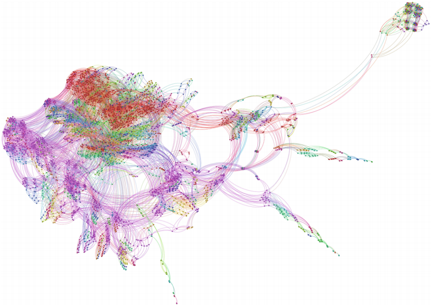Software systems. Automata models are often used to infer models of software in an unsupervised fashion, e.g. Walkinshaw et al. [2007]. In these cases, the generative property of automaton models is see as interpretable: It is possible to ask queries using a temporal logic like LTL [Clarke et al., 2005] to answer questions regarding the model, e.g. whether a certain condition will eventually be true, or analyze at what point a computation path deviated from the expected outcome. In Smetsers et al. [2016], the authors use this property to test and validate properties of code by first fuzzing the code to obtain execution paths and the associated inputs and then learn a model to check LTL queries on. Additionally, we can transfer human expert knowledge on system design [Wagner et al., 2006] to inspect the model, e.g. to identify the function of substructures identified. An example can be found in Smeenk et al. [2015], where the authors infer a state machine for a printer via active learning. Through visual inspection alone it is possible to identify deadlocks that are otherwise hard to see in the raw data. The visual analysis helped to identify bugs in the software the developers were unaware of. The appendix shows the final model in Figure 3. 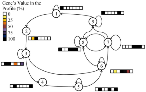Biological systems. In Schmidt and Kramer [2014], timed automata are used to infer the cell cycle of yeast based on sequences of gene expression activity. The graphical model obtained (c.f. Figure 4) can be visually compared to existing models derived using other methods and combined with a-priori knowledge in biology. 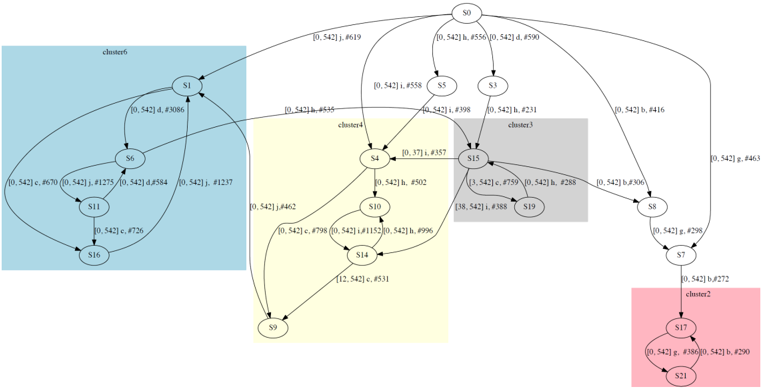Driver behavior. In our ongoing work using the RTI+ state-merging algorithm for timed automata [Verwer et al., 2008], we analyze car following behavior of human drivers. The task is to relate driver actions like changes of vehicle speed (and thus distance and relative speed to a lead vehicle) to a response action, e.g. acceleration. The inferred automaton model is inspected visually like a software controller. Different driving behaviors are distinguished by clustering the states of the automaton, i.e. the latent state space. The discovered distinct behaviors form control loops within the model. Figure 2 in the appendix shows an example with the discovered clusters highlighted. 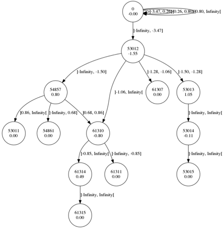Wind speed prediction. In our own work, we applied automata learning in different ways to a problem not related to grammar inference, predicting short-term changes in wind speeds. We take two different approaches to obtain models that tell us more about the data than just a minimizer of the objective function: In one approach, [Pellegrino et al., 2016], we discover structure in the data by using by inferring transition guards over a potentially infinite alphabet, effectively discovering a clustering as transition labels from the sequences automatically. The only constraint and objective used here is the similarity of future behaviors. The learned model can be seen as a structure like a decision tree built in a bottom-up fashion, but allowing loops for repetitive patterns. Figure 1 in the appendix shows an example of such an automaton. In another approach [Lin et al., 2016], we use our flexible state-merging framework to impose structure through parameter choices. We derive discrete events from the physical wind speed observations by using clustering approaches to obtain a small alphabet of discrete events as a symbolic representation that fits the underlying data well. Using a heuristic that scores merges based on minimizing a mean squared error measure, the automata model has a good objective function for regression, as well as discovers latent variables in terms of the given discretization. In practice, other choices of discretization can be used. By using thresholds of the turbine used in wind mills, e.g. the activation point, one could infer a model whose latent states relate to the physical limitations of the application. We are planning to analyze this approach in future work. As with the previous example, the learned model can be seen as a description of decision paths taken in the latent state-space. If the model makes predictions that are difficult to believe for human experts, the computation and the model prediction can be visually analyzed to see which factors contributed to it, and how the situation relates to similar sets of features. ## 6 Discussion The applications surveyed in Section 5 show that interpreting finite state automata as models takes many forms and serves different goals. As such, this interpretation is not a feature inherent in the models or the algorithms themselves. Rather, interpretations are defined by the need and intention of the user. But yet, interpretations of automata models draw from a core set of properties as identified in Section 4: graphical representations, transparent computation, generative nature, and our understanding of their theory. We note that automata models are particularly useful in unsupervised learning: Applications of automata models often aim at easing the transfer of knowledge about the subject, or related subjects, to the data generating process. In this case, machine learning serves as a tool for exploration, to deal with epistemic uncertainty in observed systems. The goal is not only to obtain a more compact view of the data, but learn how to generalize from the observed data. Often, it is often unclear what the a-priori knowledge is as users rely on experience. This makes it very difficult to formalize a clear objective function. A visual model with a traceable computation helps to guide the users, and helps to iterate over multiple models. Flexible state-merging allows to obtain automata models in new domains: in our flexible state-merging framework presented in Section 3, we try to separate the symbolic representation from the objective function and heuristic. We hope that this will help to guide discovery by stating the model parameters, e.g. the symbols, independently form the heuristic that guides the discovery of latent variables. In this fashion, it is possible to learn models with interpretable aspects without having to sacrifice the model performance on the intended task. Future work. We hope that this discussion will help to build a bridge between practitioners and experts in applied fields on one side, and the grammar inference and machine learning community on other side. As probabilistic deterministic automata models are almost as expressive as HMMs, the models and techniques described here are applicable to a wide range of problems with decent performance metrics. We see a lot of promise in combining symbolic data with numeric or other data via a flexible state-merging approach to bring automata learning to fields beyond grammatical inference. ## Acknowledgments I would like to thank, in no particular order, my colleagues, Joshua Moermann, Rick Smeters, Nino Pellegrino, Sara Messelaar, Corina Grigore, and Mijung Park for their time and feedback on this work. This work is partially funded by the FNR AFR grant PAULINE and Technologiestichting STW VENI project 13136 (MANTA) and NWO project 62001628 (LEMMA). ## References - Dana Angluin. Learning Regular Sets from Queries and Counterexamples. Information and Computation , 75(2): 87-106, 1987. URL http://dx.doi.org/10.1016/0890-5401(87)90052-6 . - Borja Balle, Xavier Carreras, Franco M. Luque, and Ariadna Quattoni. Spectral Learning of Weighted Automata. Machine Learning , 96(1-2):33-63, 2014. URL http://link.springer.com/article/10.1007/ s10994-013-5416-x . - Edmund Clarke, Ansgar Fehnker, Sumit Kumar Jha, and Helmut Veith. Temporal Logic Model Checking. In Handbook of Networked and Embedded Control Systems , Control Engineering, pages 539-558. Birkhäuser Boston, 2005. ISBN 978-0-8176-3239-7 978-0-8176-4404-8. URL http://link.springer. com/chapter/10.1007/0-8176-4404-0\_23 . - Madalina Fiterau, Artur Dubrawski, Jeff Schneider, and Geoff Gordon. Trade-offs in Explanatory Model Learning. 2012. URL http://www.ml.cmu.edu/research/dap-papers/dap\_fiterau.pdf . - Marta Garnelo, Kai Arulkumaran, and Murray Shanahan. Towards Deep Symbolic Reinforcement Learning. arXiv:1609.05518 [cs] , September 2016. URL http://arxiv.org/abs/1609.05518 . arXiv: 1609.05518. - Bryce Goodman and Seth Flaxman. European Union Regulations on Algorithmic Decision-making and a "Right to Explanation". arXiv:1606.08813 [cs, stat] , June 2016. URL http://arxiv.org/abs/1606.08813 . arXiv: 1606.08813. - Colin de la Higuera. Grammatical Inference: Learning Automata and Grammars . Cambridge University Press, April 2010. ISBN 978-0-521-76316-5. - John E. Hopcroft, Rajeev Motwani, and Jeffrey D. Ullman. Introduction to Automata Theory, Languages, and Computation . Pearson, Harlow, Essex, Pearson New International Edition edition, November 2013. ISBN 978-1-292-03905-3. - D. Lee and M. Yannakakis. Principles and Methods of Testing Finite State Machines-a Survey. Proceedings of the IEEE , 84(8):1090-1123, August 1996. ISSN 0018-9219. doi: 10.1109/5.533956. - Qin Lin, Christian Hammerschmidt, Gaetano Pellegrino, and Sicco Verwer. Short-term Time Series Forecasting with Regression Automata. In MiLeTS Workshop at KDD 2016 , 2016. URL http://www-bcf.usc.edu/ ~liu32/milets16/paper/MiLeTS\_2016\_paper\_17.pdf . - Zachary C. Lipton. The Mythos of Model Interpretability. arXiv:1606.03490 [cs, stat] , June 2016. URL http://arxiv.org/abs/1606.03490 . arXiv: 1606.03490. - Jose Oncina and Pedro Garcia. Identifying Regular Languages In Polynomial Time. In Advances in Structural and Syntactic Pattern Recognition , pages 99-108. World Scientific, 1992. - Gaetano Pellegrino, Christian Albert Hammerschmidt, Qin Lin, and Sicco Verwer. Learning Deterministic Finite Automata from Infinite Alphabets. In Proceedings of The 13th International Conference on Grammatical Inference , Delft, October 2016. - Jana Schmidt and Stefan Kramer. Online Induction of Probabilistic Real-Time Automata. Journal of Computer Science and Technology , 29(3):345-360, May 2014. ISSN 1000-9000, 1860-4749. doi: 10.1007/ s11390-014-1435-8. URL http://link.springer.com/article/10.1007/s11390-014-1435-8 . - Wouter Smeenk, Joshua Moerman, Frits Vaandrager, and David N. Jansen. Applying Automata Learning to Embedded Control Software. In Formal Methods and Software Engineering , number 9407 in Lecture Notes in Computer Science, pages 67-83. November 2015. URL http://link.springer.com/chapter/10. 1007/978-3-319-25423-4\_5 . - Rick Smetsers, Joshua Moerman, Mark Janssen, and Sicco Verwer. Complementing Model Learning with Mutation-Based Fuzzing. arXiv:1611.02429 [cs] , 2016. URL http://arxiv.org/abs/1611.02429 . arXiv: 1611.02429. - Ryan Turner. A Model Explanation System. In Black Box Learning and Inference NIPS Workshop , 2015. URL http://www.blackboxworkshop.org/pdf/Turner2015\_MES.pdf . - Wil Van Der Aalst, Arya Adriansyah, Ana Karla Alves de Medeiros, Franco Arcieri, Thomas Baier, Tobias Blickle, Jagadeesh Chandra Bose, Peter van den Brand, Ronald Brandtjen, Joos Buijs, and others. Process Mining Manifesto. In Business Process Management Workshops , pages 169-194. Springer, 2012. URL http://link.springer.com/chapter/10.1007/978-3-642-28108-2\_19 . - Sicco Verwer, Mathijs de Weerdt, and Cees Witteveen. Efficiently Learning Simple Timed Automata. Induction of Process Models , pages 61-68, 2008. URL http://www.cs.ru.nl/~sicco/papers/ipm08.pdf . - Ferdinand Wagner, Ruedi Schmuki, Thomas Wagner, and Peter Wolstenholme. Modeling Software with Finite State Machines: A Practical Approach . CRC Press, May 2006. ISBN 978-1-4200-1364-1. - N. Walkinshaw, K. Bogdanov, M. Holcombe, and S. Salahuddin. Reverse Engineering State Machines by Interactive Grammar Inference. In 14th Working Conference on Reverse Engineering (WCRE 2007) , 2007. 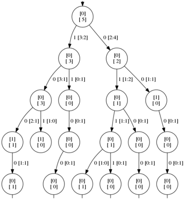## A Visualizations of Automata Figure 1: Auto-regressive model of short-term average wind speeds using the approach presented by Lin et al. [2016]. The ranges on the transitions indicate for which speed they activate, the number in the nodes is the predicted change in speed. The top node models persistent behavior (i.e. no change in speed for the next period), whereas the lower part denotes exceptions to this rule. <details> <summary>Image 1 Details</summary>  ### Visual Description ## Directed Graph: State Transition Diagram ### Overview The image depicts a directed graph, likely representing a state transition diagram. Each node represents a state, labeled with a numerical identifier and a value. The edges between nodes represent transitions, with each edge labeled with an interval. ### Components/Axes * **Nodes:** Represented as circles, each containing two lines of text: * A numerical identifier (e.g., 0, 53012, 54857). * A numerical value (e.g., -0.00, -1.55, 0.80). * **Edges:** Represented as arrows, indicating the direction of the transition. Each edge is labeled with an interval, enclosed in square brackets (e.g., `[-3.47, 0.26]`, `[-Infinity, -3.47]`). * **Root Node:** The node labeled "0" with a value of "-0.00" is at the top of the diagram. ### Detailed Analysis Here's a breakdown of the nodes and their connections, including the interval labels on the edges: * **Node 0:** * Identifier: 0 * Value: -0.00 * Outgoing edge to itself: `[-3.47, 0.26]`, `[0.26, 0.80]`, `[0.80, Infinity]` * Outgoing edge to Node 53012: `[-Infinity, -3.47]` * **Node 53012:** * Identifier: 53012 * Value: -1.55 * Outgoing edge to Node 54857: `[-Infinity, -1.50]` * Outgoing edge to Node 61307: `[-1.28, -1.06]` * Outgoing edge to Node 53013: `[-1.50, -1.28]` * Outgoing edge to Node 61310: `[-1.06, Infinity]` * **Node 54857:** * Identifier: 54857 * Value: 0.80 * Outgoing edge to Node 53011: `[0.86, Infinity]` * Outgoing edge to Node 54861: `[-Infinity, 0.68]` * Outgoing edge to Node 61310: `[0.68, 0.86]` * **Node 61307:** * Identifier: 61307 * Value: 0.00 * No outgoing edges. * **Node 53013:** * Identifier: 53013 * Value: 1.05 * Outgoing edge to Node 53014: `[-Infinity, Infinity]` * **Node 61310:** * Identifier: 61310 * Value: -0.80 * Outgoing edge to Node 61314: `[-0.85, Infinity]` * Outgoing edge to Node 61311: `[-Infinity, -0.85]` * **Node 53011:** * Identifier: 53011 * Value: 0.00 * No outgoing edges. * **Node 54861:** * Identifier: 54861 * Value: 0.00 * No outgoing edges. * **Node 61314:** * Identifier: 61314 * Value: 0.49 * Outgoing edge to Node 61315: `[-Infinity, Infinity]` * **Node 61311:** * Identifier: 61311 * Value: 0.00 * No outgoing edges. * **Node 53014:** * Identifier: 53014 * Value: -0.11 * Outgoing edge to Node 53015: `[-Infinity, Infinity]` * **Node 61315:** * Identifier: 61315 * Value: 0.00 * No outgoing edges. * **Node 53015:** * Identifier: 53015 * Value: 0.00 * No outgoing edges. ### Key Observations * Node 0 is the root and has a self-loop. * The edges are labeled with intervals, suggesting conditions or probabilities for the transitions. * Several nodes (53011, 54861, 61307, 61311, 61315, 53015) are terminal nodes, having no outgoing edges. * Some edges have intervals that include infinity, indicating unbounded conditions. ### Interpretation The diagram likely represents a state machine or a decision tree. The numerical values associated with each node could represent a cost, a probability, or some other relevant metric for that state. The intervals on the edges define the conditions under which a transition from one state to another occurs. The self-loop on Node 0 suggests that the system can remain in the initial state under certain conditions. The terminal nodes represent final states or outcomes. The intervals on the edges could represent ranges of values for a variable that determines the transition. The use of infinity in some intervals suggests that the transition is possible for all values above or below a certain threshold. </details> Figure 2: Car-following controller model with highlighted clusters. Each color denotes one distinct cluster. The loop in cluster 6 (colored light blue), e.g. state sequence: 1-6-11-16-1 with symbolic transitions loop: d (keep short distance and slower than lead vehicle)-j (keep short distance and same speed to lead vehicle)-c (keep short distance and faster than lead vehicle))-j, can be interpreted as the car-following behavior at short distances , i.e. adapting the speed difference with the lead vehicle around 0 and bounding the relative distance in small zone. Similarly interesting and significant loops can be also seen in cluster 2 (colored pink) and cluster 4 (colored light yellow), which are long distance and intermediate distance car-following behaviors respectively. The intermediate state like S 15 in cluster 3 (colored light grey) explains how to switch between clusters. <details> <summary>Image 2 Details</summary>  ### Visual Description ## State Transition Diagram: Cluster Analysis ### Overview The image is a state transition diagram, visually representing the relationships and transitions between different states (S0 to S21). The diagram is divided into clusters, each highlighted with a different background color. Transitions between states are labeled with probabilities and identifiers. ### Components/Axes * **Nodes:** Represented by circles labeled S0, S1, S3, S4, S5, S6, S7, S8, S9, S10, S11, S14, S15, S16, S17, S19, S21. * **Edges:** Represented by arrows indicating transitions between states. Each arrow is labeled with transition probabilities and identifiers, in the format `[probability] letter, #identifier`. * **Clusters:** The diagram is divided into clusters, each with a distinct background color: * Cluster 6: Light blue, containing nodes S1, S6, S11, and S16. * Cluster 4: Light yellow, containing nodes S4, S9, S10, and S14. * Cluster 3: Light gray, containing nodes S15 and S19. * Cluster 2: Light red, containing nodes S7, S17, and S21. * **Labels:** Each node is labeled with an "S" followed by a number (e.g., S0, S1, S2). Edges are labeled with transition probabilities and identifiers. ### Detailed Analysis or Content Details * **Node S0:** * Transitions to S1 with label `[0.542] j, #619`. * Transitions to S3 with label `[0.542] d, #590`. * Transitions to S5 with label `[0.542] h, #556`. * Transitions to S8 with label `[0.542] b, #416`. * **Node S1:** * Transitions to S6 with label `[0.542] d, #3086`. * **Node S3:** * Transitions to S15 with label `[0.542] i, #231`. * **Node S4:** * Transitions to S15 with label `[0.37] i, #357`. * Transitions to S10 with label `[0.542] h, #502`. * Transitions to S9 with label `[0.542] j, #462`. * Transitions to S1 with label `[0.542] b, #535`. * **Node S5:** * Transitions to S4 with label `[0.542] i, #558`. * **Node S6:** * Transitions to S11 with label `[0.542] c, #670`. * Transitions to S11 with label `[0.542] j, #1275`. * Transitions to S1 with label `[0.542] d, #584`. * Transitions to S1 with label `[0.542] j, #1237`. * **Node S7:** * Transitions to S17 with label `[0.542] b, #272`. * **Node S8:** * Transitions to S7 with label `[0.542] g, #298`. * Transitions to S15 with label `[0.542] b, #306`. * **Node S9:** * Transitions to S0 with label `[0.542] g, #463`. * **Node S10:** * Transitions to S14 with label `[0.542] c, #798`. * Transitions to S14 with label `[0.542] i, #1152`. * Transitions to S14 with label `[0.542] h, #996`. * **Node S11:** * Transitions to S16 with label `[0.542] c, #726`. * **Node S14:** * Transitions to S9 with label `[12.542] c, #531`. * **Node S15:** * Transitions to S19 with label `[38, 542] i, #388`. * Transitions to S19 with label `[3, 542] c, #759`. * Transitions to S19 with label `[0.542] h, #288`. * **Node S17:** * Transitions to S21 with label `[0.542] g, #386`. * Transitions to S21 with label `[0.542] b, #290`. * **Node S21:** * Transitions to S17 with label `[0.542] g, #386`. * Transitions to S17 with label `[0.542] b, #290`. ### Key Observations * The diagram represents a complex state machine with multiple interconnected states. * The clusters visually group related states, potentially indicating functional or behavioral similarities. * Transition probabilities are consistently around 0.542, with a few exceptions (0.37 and 12.542). * Nodes S17 and S21 form a self-loop within cluster 2. ### Interpretation The state transition diagram likely models the behavior of a system or process. The clusters could represent different modes of operation or functional units within the system. The transition probabilities indicate the likelihood of moving from one state to another. The identifiers associated with each transition could represent specific events or conditions that trigger the transition. The self-loop between S17 and S21 suggests a stable or recurring state within cluster 2. The diagram provides a visual representation of the system's dynamics and can be used to analyze its behavior and identify potential issues or areas for optimization. </details> Figure 3: Visualization of a state machine learned from a printer controller using an active learning approach. Each state, represented as a dot, represents a state in the controller software and each transition, represened as an edge, a state-change upon receiving input. Using knowledge about the controller design, it is possible to identify the sparsely connected protrusions of states at the bottom as deadlock situations. Taken from Smeenk et al. [2015] <details> <summary>Image 3 Details</summary>  ### Visual Description ## Network Diagram: Complex Interconnected System ### Overview The image presents a complex network diagram with numerous nodes and edges. The nodes are represented by small colored circles, and the edges are represented by curved lines connecting these nodes. The diagram exhibits a high degree of interconnectedness, with a dense cluster of nodes in the central-left region and sparser clusters extending outwards. The colors of the nodes and edges vary, suggesting different categories or properties within the network. ### Components/Axes * **Nodes:** Represented by small colored circles. The colors include red, green, blue, purple, and variations thereof. * **Edges:** Represented by curved lines connecting the nodes. The colors of the edges generally match the colors of the nodes they connect. * **Clusters:** The nodes are grouped into several clusters, with a large, dense cluster in the central-left region and smaller, more dispersed clusters extending towards the right. ### Detailed Analysis * **Central-Left Cluster:** This is the most prominent feature of the diagram. It is a dense aggregation of nodes with a mix of colors, including red, green, blue, and purple. The edges within this cluster are highly interconnected, forming a complex web. * **Rightward Extensions:** Several sparser clusters extend from the central-left cluster towards the right. These clusters are less dense and more elongated, with fewer interconnections. The colors of the nodes and edges in these extensions vary, suggesting different sub-networks or pathways. * **Color Distribution:** The color distribution appears to be non-random. The red nodes seem to be concentrated in the upper part of the central-left cluster, while the purple nodes are more prevalent in the lower part. The green and blue nodes are interspersed throughout the cluster. * **Isolated Cluster (Top-Right):** There is a distinct, relatively isolated cluster in the top-right corner of the diagram. This cluster is connected to the main network by a few long edges. ### Key Observations * The network exhibits a core-periphery structure, with a dense core in the central-left region and sparser periphery extending outwards. * The color-coding of the nodes and edges suggests different categories or properties within the network. * The isolated cluster in the top-right corner may represent a distinct sub-network or module. ### Interpretation The network diagram likely represents a complex system with multiple interacting components. The dense central cluster may represent a core set of entities or processes, while the sparser extensions represent peripheral elements or pathways. The color-coding could indicate different types of entities, relationships, or states within the system. The isolated cluster in the top-right corner may represent a specialized module or subsystem. Without further context or a legend, it is difficult to determine the specific meaning of the nodes, edges, and colors. However, the diagram provides a visual representation of the system's structure and interconnectedness, which can be useful for understanding its overall behavior and identifying key areas for further investigation. </details> . Figure 4: The yeast cell cycle learned in Schmidt and Kramer [2014] using a passive online learning algorithm for timed automata. The colored bars indicate gene activities. The model corresponds to the well-known yeast cycle. <details> <summary>Image 4 Details</summary>  ### Visual Description ## Diagram: Gene Regulatory Network with Expression Profiles ### Overview The image depicts a gene regulatory network diagram. The network consists of nine nodes, each representing a gene, interconnected by directed edges indicating regulatory relationships. Each node is associated with a bar graph representing the gene's expression profile, with colors indicating the gene's value in the profile, ranging from 0% (white) to 100% (black). ### Components/Axes * **Nodes:** Numbered 1 through 9, representing individual genes. * **Edges:** Directed arrows indicating regulatory relationships between genes. * **Expression Profiles:** Bar graphs associated with each node, showing the gene's value in the profile. * **Color Legend (Left):** * White: 0% * Light Yellow: 25% * Orange: 50% * Brown: 75% * Dark Blue/Purple: 75% * Black: 100% ### Detailed Analysis Here's a breakdown of each node and its associated expression profile: * **Node 1:** Has a self-loop. The expression profile is mostly black, indicating a high gene value (approximately 100%) across most of the profile, with a single white block. * **Node 2:** Receives an edge from Node 1 and sends an edge to Node 3. The expression profile shows a light yellow block, followed by a black block, and then white blocks. This indicates a gene value of approximately 25% followed by 100% and then 0%. * **Node 3:** Receives edges from Nodes 2 and 4 and has a self-loop. The expression profile shows black, light yellow, orange, and dark blue/purple blocks, followed by white blocks. This corresponds to values of approximately 100%, 25%, 50%, 75%, and 0%. * **Node 4:** Receives an edge from Node 3 and sends an edge to Node 5. The expression profile is mostly black, indicating a high gene value (approximately 100%) across most of the profile, with a single white block. * **Node 5:** Receives an edge from Node 4 and sends an edge to Node 6. The expression profile is mostly black, indicating a high gene value (approximately 100%) across most of the profile, with a single white block. * **Node 6:** Receives edges from Nodes 3 and 5 and sends edges to Nodes 7 and 8. It also has a self-loop. The expression profile shows light yellow, black, and brown blocks, followed by white blocks. This corresponds to values of approximately 25%, 100%, 75%, and 0%. * **Node 7:** Receives edges from Node 6 and sends edges to Nodes 8 and 9. It also has a self-loop. The expression profile is mostly black, indicating a high gene value (approximately 100%) across most of the profile, with a single white block. * **Node 8:** Receives edges from Nodes 6 and 7 and sends edges to Nodes 7 and 9. The expression profile is mostly black, indicating a high gene value (approximately 100%) across most of the profile, with a single white block. * **Node 9:** Receives edges from Nodes 7 and 8 and sends an edge to Node 1. It also has a self-loop. The expression profile is mostly black, indicating a high gene value (approximately 100%) across most of the profile, with a single white block. ### Key Observations * Nodes 1, 3, 6, 7, 8, and 9 have self-loops, suggesting autoregulation. * Nodes 7 and 8 form a bidirectional regulatory loop. * Nodes 1, 4, 5, 7, 8, and 9 have expression profiles that are predominantly black, indicating high gene values. * Nodes 2, 3, and 6 have more diverse expression profiles, suggesting more dynamic regulation. ### Interpretation The diagram represents a gene regulatory network, where nodes represent genes and edges represent regulatory interactions. The expression profiles associated with each gene provide information about the gene's activity level under specific conditions or at different time points. The network structure and expression profiles suggest complex regulatory relationships between the genes. The presence of self-loops indicates autoregulation, while the bidirectional loop between Nodes 7 and 8 suggests a feedback mechanism. The varying expression profiles indicate that some genes are more dynamically regulated than others. The network could be used to model and understand the behavior of a biological system, such as a cell or an organism. </details> ## B Finite State Automata In this section, we give a formal introduction to deterministic finite state automata as the most basic model considered in the related work. For other variants like probabilistic automata, timed and real time automata, and regression automata, we refer to the cited papers for formal introductions. A deterministic finite state automaton (DFA) is one of the basic and most commonly used finite state machines. Below, we provide a concise description of DFAs, the reader is referred to Hopcroft et al. [2013] for a more elaborate overview. A DFA A = 〈 Q,T, Σ , q 0 , Q + 〉 is a directed graph consisting of a set of states Q (nodes) and labeled transitions T (directed edges). An example is shown in Figure 6. The start state q 0 ∈ Q is a specific state of the DFA and any state can be an accepting state (final state) in Q + ⊆ Q . The labels of transitions are all members of a given alphabet Σ . A DFA A can be used to generate or accept sequences of symbols (strings) using a process called DFA computation . This process begins in q 0 , and iteratively activates (or fires ) an outgoing transition t i = 〈 q i -1 , q i , l i 〉 ∈ T with label l i ∈ Σ from the source state it is in q i -1 , moving the process to the target state q i pointed to by t i . A computation q 0 t 1 q 1 t 2 q 2 . . . t n q n is accepting if the state it ends in (its last state) is an accepting state q n ∈ Q + , otherwise it is rejecting . The labels of the activated transitions form a string l 1 . . . l n . A DFA accepts exactly those strings formed by the labels of accepting computations, it rejects all others. Since a DFA is deterministic there exists exactly one computation for every string, implying that for every state q and every label l there exists at most one outgoing transition from q with label l . A string s is said to reach all the states contained in the computation that forms s , s is said to end in the last state q n of such a computation. The set of all strings accepted by a DFA A is called the language L ( A ) of A . Figure 5: The initial part of the prefix tree, built from the input sample as shown in Figure 7. The square brackets indicate occurrence counts of positive data. <details> <summary>Image 5 Details</summary>  ### Visual Description ## Decision Tree: Binary Classification ### Overview The image depicts a binary decision tree. Each node represents a decision point, and the edges represent the outcomes of those decisions (0 or 1). The nodes contain two values, the first is always 0 or 1, and the second is a count. The tree structure shows how data is split based on binary features, leading to classifications at the leaf nodes. ### Components/Axes * **Nodes:** Each node is represented by a circle containing two bracketed values: `[x]` and `[y]`. The first value `x` is either `0` or `1`. The second value `y` is an integer representing a count. * **Edges:** Edges connect the nodes, indicating the flow of decisions. Each edge is labeled with a binary value (0 or 1) and a ratio `[a:b]`. The first value `a` is the binary value of the edge. The second value `b` is a count. * **Root Node:** Located at the top of the tree. * **Leaf Nodes:** Located at the bottom of the tree. ### Detailed Analysis * **Root Node:** The root node at the top has the values `[0]` and `[5]`. * The edge to the left child is labeled `1 [3:2]`. * The edge to the right child is labeled `0 [2:4]`. * **Level 1 Nodes:** * Left child of the root node has the values `[0]` and `[3]`. * Right child of the root node has the values `[0]` and `[2]`. * **Level 2 Nodes (Left Subtree):** * Left child of the `[0][3]` node has the values `[0]` and `[3]`. The edge is labeled `0 [3:1]`. * Right child of the `[0][3]` node has the values `[0]` and `[0]`. The edge is labeled `1 [0:1]`. * **Level 2 Nodes (Right Subtree):** * Left child of the `[0][2]` node has the values `[0]` and `[1]`. The edge is labeled `1 [1:2]`. * Right child of the `[0][2]` node has the values `[1]` and `[0]`. The edge is labeled `0 [1:1]`. * **Level 3 Nodes (Left-Left Subtree):** * Left child of the `[0][3]` node has the values `[1]` and `[1]`. The edge is labeled `0 [2:1]`. * Right child of the `[0][3]` node has the values `[1]` and `[0]`. The edge is labeled `1 [1:0]`. * **Level 3 Nodes (Left-Right Subtree):** * The child of the `[0][0]` node has the values `[0]` and `[0]`. The edge is labeled `0 [0:1]`. * **Level 3 Nodes (Right-Left Subtree):** * Left child of the `[0][1]` node has the values `[0]` and `[1]`. The edge is labeled `1 [1:1]`. * Right child of the `[0][1]` node has the values `[0]` and `[0]`. The edge is labeled `0 [0:1]`. * **Level 3 Nodes (Right-Right Subtree):** * The child of the `[1][0]` node has the values `[0]` and `[0]`. The edge is labeled `0 [0:1]`. * **Level 4 Nodes:** All leaf nodes at this level have the values `[0]` and `[0]` or `[0]` and `[1]`. * The child of the `[1][1]` node has the values `[0]` and `[1]`. The edge is labeled `0 [1:1]`. * The child of the `[1][0]` node has the values `[0]` and `[0]`. The edge is labeled `0 [0:1]`. * Left child of the `[0][1]` node has the values `[0]` and `[0]`. The edge is labeled `1 [1:0]`. * Right child of the `[0][1]` node has the values `[0]` and `[0]`. The edge is labeled `0 [0:1]`. * The child of the `[0][0]` node has the values `[0]` and `[0]`. The edge is labeled `0 [0:1]`. * The child of the `[0][0]` node has the values `[0]` and `[0]`. The edge is labeled `0 [0:1]`. ### Key Observations * The tree is binary, meaning each node has at most two children. * The values within the nodes and on the edges seem to represent counts or probabilities associated with each decision path. * The tree is not perfectly balanced, as some branches are deeper than others. * The leaf nodes predominantly have a first value of `0`. ### Interpretation The decision tree likely represents a classification model where binary features are used to predict a binary outcome (0 or 1). The counts within the nodes and on the edges could represent the number of samples that follow a particular decision path. The tree structure shows how the data is split based on these features, and the leaf nodes represent the final classifications. The imbalance in the tree suggests that some features are more informative than others in making the classification decision. The prevalence of `0` as the first value in the leaf nodes might indicate a bias towards predicting the `0` class. 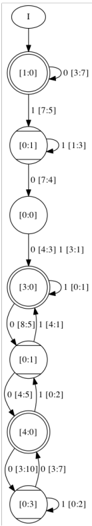</details> Figure 6: An automaton learned from the input sample. The numbers in square brackets indicate occurrence counts of positive and negative samples. <details> <summary>Image 6 Details</summary>  ### Visual Description ## State Diagram: Finite State Machine ### Overview The image depicts a state diagram, representing a finite state machine. It consists of nodes representing states and directed edges representing transitions between states, labeled with input values and associated data. ### Components/Axes * **Nodes:** Represent states, labeled with bracketed numbers (e.g., [1:0], [0:1], [0:0], [3:0], [4:0], [0:3]). The node labeled [1:0], [3:0], and [4:0] are double-circled, indicating accepting states. * **Edges:** Represent transitions between states, labeled with an input value (0 or 1) and associated data in brackets (e.g., 0 [3:7], 1 [7:5]). * **Start State:** The state labeled "1" at the top of the diagram is the start state. ### Detailed Analysis or ### Content Details 1. **Start State:** * Node: 1 * Transition to [1:0]: Unlabeled arrow. 2. **State [1:0]:** * Node: [1:0] (Accepting State) * Transition to [0:1]: 1 [7:5] * Self-loop: 0 [3:7] 3. **State [0:1]:** * Node: [0:1] * Transition to [0:0]: 0 [7:4] * Self-loop: 1 [1:3] 4. **State [0:0]:** * Node: [0:0] * Transition to [3:0]: 0 [4:3] * Transition to [3:0]: 1 [3:1] 5. **State [3:0]:** * Node: [3:0] (Accepting State) * Self-loop: 1 [0:1] * Transition to [0:1]: 0 [8:5] * Transition to [0:1]: 1 [4:1] 6. **State [4:0]:** * Node: [4:0] (Accepting State) * Transition to [0:3]: 0 [3:10] * Transition to [0:3]: 0 [3:7] 7. **State [0:3]:** * Node: [0:3] * Self-loop: 1 [0:2] 8. **State [4:0]:** * Node: [4:0] * Transition to [0:1]: 0 [4:5] * Transition to [0:1]: 1 [0:2] ### Key Observations * The diagram represents a finite state machine with 7 states (excluding the initial state "1"). * States [1:0], [3:0], and [4:0] are accepting states. * Transitions are labeled with input values (0 or 1) and associated data. * Self-loops exist in states [1:0], [0:1], [3:0], and [0:3]. ### Interpretation The state diagram illustrates the behavior of a finite state machine. The machine transitions between states based on input values, and the accepting states indicate successful or valid outcomes. The data associated with each transition could represent costs, probabilities, or other relevant information for each state transition. The specific meaning of the bracketed numbers within the states and transitions is not clear from the diagram alone, but they likely represent some form of state or transition metadata. </details> ## C State-Merging Algorithms The idea of a state-merging algorithm is to first construct a tree-shaped DFA A from the input sample S , and then to merge the states of A . This DFA A is called an augmented prefix tree acceptor (APTA). An example is shown in Figure 5. For every state q of A , there exists exactly one computation that ends in q . This implies that the computations of two strings s and s ′ reach the same state q if and only if s and s ′ share the same prefix until they reach q . Furthermore, an APTA A is constructed to be consistent with the input sample S , i.e., S + ⊆ L ( A ) and S -∩ L ( A ) = ∅ . Thus a state q is accepting only if there exists a string s ∈ S + such that the computation of s ends in q . Similarly, it is rejecting only if the computation of a string s ∈ S -ends in q . As a consequence, A can contain states that are neither accepting nor rejecting. No computation of any string from S ends in such a state. Therefore, the rejecting states are maintained in a separate set Q -⊆ Q , with Q -∪ Q + = ∅ . Whether a state q ∈ Q \ ( Q + ∪ Q -) should be accepting or rejecting is determined by merging the states of the APTA and trying to find a DFA that is as small as possible. 1 9 1 0 0 0 0 0 0 0 0 1 15 0 1 1 0 0 0 1 0 1 0 1 0 1 0 0 0 5 0 1 0 0 0 1 2 0 0 0 12 1 1 0 0 0 0 0 0 0 1 0 0 1 5 1 0 1 0 0 1 3 1 0 0 0 6 0 0 0 0 0 1 1 3 1 0 1 0 20 1 0 0 0 0 0 1 0 1 0 0 0 0 0 1 1 1 0 0 0 0 13 0 1 1 1 0 1 0 0 0 0 0 0 0 1 3 1 0 1 1 7 1 0 0 0 0 0 0 Figure 7: Input sample for the APTA in Figure 5 and the learned model in Figure 6. The first column indicates whether the sample is positive or negative (i.e. a counter-example), the second column indicates the length of the word. The following symbols form the word, with each symbol separated by a space. This input format is commonly used in tools in the grammar induction community. A merge of two states q and q ′ combines the states into one: it creates a new state q ′′ that has the incoming and outgoing transitions of both q and q ′ , i.e., replace all 〈 q, q t , l 〉 , 〈 q ′ , q t , l 〉 ∈ T by 〈 q ′′ , q t , l 〉 and all 〈 q s , q, l 〉 , 〈 q s , q ′ , l 〉 ∈ T by 〈 q s , q ′′ , l 〉 . Such a merge is only allowed if the states are consistent , i.e., it is not the case that q is accepting while q ′ is rejecting or vice versa. When a merge introduces a non-deterministic choice, i.e., q ′′ is now the source of two transitions 〈 q ′′ , q 1 , l 〉 and 〈 q ′′ , q 2 , l 〉 in T with the same label l , the target states of these transitions q 1 and q 2 are merged as well. This is called the determinization process (c.f. the while-loop in Algorithm 2), and is continued until there are no non-deterministic choices left. However, if this process at some point merges two inconsistent states, the original states q and q ′ are also considered inconsistent and the merge will fail. The result of a successful merge is a new DFA that is smaller than before, and still consistent with the input sample S . A state-merging algorithm iteratively applies this state merging process until no more consistent merges are possible. The general algorithm is outlined in Algorithm 1. Figure 6 shows an automaton obtained from the input given in Figure 7, which is also depicted as an APTA in Figure 5. ``` <loc_0><loc_0><loc_500><loc_499><_FORTRAN_>Algorithm 1 State-merging in the red-blue framework Require: an input sample S Ensure: A is a DFA that is consistent with S A = apta(S) {construct the APTA A} R = {q0} {color the start state of A red} B = {q \ Q \ R | \exists \ q0, q, l \ } T {color all its children blue} while B # 0 do {while A contains blue states} if \b \in B s.t. \r \in R holds merge (A, r, b) = FALSE then {if there is a blue state inconsistent with every red state} R := R \{ b} B := B \{ q \in Q \ R | \exists \langle b, q, l \rangle \ } T {color all its children blue} else for all b \in B and r \in R do {forall red-blue pair of states} compute the evidence (A, q, q') of merge (A, r, b) {find the best performing merge} end for A := merge (A, r, b) with highest evidence {perform the best merge} let q'' be resulting state R := R \{q''} {color the resulting state red} R := R \{r} {uncolor the merged red state} B := {q \ Q \ R | \exists r \in R and \langle r, q, l \rangle \ } T {recompute the set of blue states} end if end while return A ``` ``` ``` ``` end if end while return A ```