## Model-Agnostic Meta-Learning for Fast Adaptation of Deep Networks
Chelsea Finn 1 Pieter Abbeel 1 2 Sergey Levine 1
## Abstract
We propose an algorithm for meta-learning that is model-agnostic, in the sense that it is compatible with any model trained with gradient descent and applicable to a variety of different learning problems, including classification, regression, and reinforcement learning. The goal of meta-learning is to train a model on a variety of learning tasks, such that it can solve new learning tasks using only a small number of training samples. In our approach, the parameters of the model are explicitly trained such that a small number of gradient steps with a small amount of training data from a new task will produce good generalization performance on that task. In effect, our method trains the model to be easy to fine-tune. We demonstrate that this approach leads to state-of-the-art performance on two fewshot image classification benchmarks, produces good results on few-shot regression, and accelerates fine-tuning for policy gradient reinforcement learning with neural network policies.
## 1. Introduction
Learning quickly is a hallmark of human intelligence, whether it involves recognizing objects from a few examples or quickly learning new skills after just minutes of experience. Our artificial agents should be able to do the same, learning and adapting quickly from only a few examples, and continuing to adapt as more data becomes available. This kind of fast and flexible learning is challenging, since the agent must integrate its prior experience with a small amount of new information, while avoiding overfitting to the new data. Furthermore, the form of prior experience and new data will depend on the task. As such, for the greatest applicability, the mechanism for learning to learn (or meta-learning) should be general to the task and
1 University of California, Berkeley 2 OpenAI. Correspondence to: Chelsea Finn < cbfinn@eecs.berkeley.edu > .
Proceedings of the 34 th International Conference on Machine Learning , Sydney, Australia, PMLR 70, 2017. Copyright 2017 by the author(s).
the form of computation required to complete the task.
In this work, we propose a meta-learning algorithm that is general and model-agnostic, in the sense that it can be directly applied to any learning problem and model that is trained with a gradient descent procedure. Our focus is on deep neural network models, but we illustrate how our approach can easily handle different architectures and different problem settings, including classification, regression, and policy gradient reinforcement learning, with minimal modification. In meta-learning, the goal of the trained model is to quickly learn a new task from a small amount of new data, and the model is trained by the meta-learner to be able to learn on a large number of different tasks. The key idea underlying our method is to train the model's initial parameters such that the model has maximal performance on a new task after the parameters have been updated through one or more gradient steps computed with a small amount of data from that new task. Unlike prior meta-learning methods that learn an update function or learning rule (Schmidhuber, 1987; Bengio et al., 1992; Andrychowicz et al., 2016; Ravi & Larochelle, 2017), our algorithm does not expand the number of learned parameters nor place constraints on the model architecture (e.g. by requiring a recurrent model (Santoro et al., 2016) or a Siamese network (Koch, 2015)), and it can be readily combined with fully connected, convolutional, or recurrent neural networks. It can also be used with a variety of loss functions, including differentiable supervised losses and nondifferentiable reinforcement learning objectives.
The process of training a model's parameters such that a few gradient steps, or even a single gradient step, can produce good results on a new task can be viewed from a feature learning standpoint as building an internal representation that is broadly suitable for many tasks. If the internal representation is suitable to many tasks, simply fine-tuning the parameters slightly (e.g. by primarily modifying the top layer weights in a feedforward model) can produce good results. In effect, our procedure optimizes for models that are easy and fast to fine-tune, allowing the adaptation to happen in the right space for fast learning. From a dynamical systems standpoint, our learning process can be viewed as maximizing the sensitivity of the loss functions of new tasks with respect to the parameters: when the sensitivity is high, small local changes to the parameters can lead to
large improvements in the task loss.
The primary contribution of this work is a simple modeland task-agnostic algorithm for meta-learning that trains a model's parameters such that a small number of gradient updates will lead to fast learning on a new task. We demonstrate the algorithm on different model types, including fully connected and convolutional networks, and in several distinct domains, including few-shot regression, image classification, and reinforcement learning. Our evaluation shows that our meta-learning algorithm compares favorably to state-of-the-art one-shot learning methods designed specifically for supervised classification, while using fewer parameters, but that it can also be readily applied to regression and can accelerate reinforcement learning in the presence of task variability, substantially outperforming direct pretraining as initialization.
## 2. Model-Agnostic Meta-Learning
We aim to train models that can achieve rapid adaptation, a problem setting that is often formalized as few-shot learning. In this section, we will define the problem setup and present the general form of our algorithm.
## 2.1. Meta-Learning Problem Set-Up
The goal of few-shot meta-learning is to train a model that can quickly adapt to a new task using only a few datapoints and training iterations. To accomplish this, the model or learner is trained during a meta-learning phase on a set of tasks, such that the trained model can quickly adapt to new tasks using only a small number of examples or trials. In effect, the meta-learning problem treats entire tasks as training examples. In this section, we formalize this metalearning problem setting in a general manner, including brief examples of different learning domains. We will discuss two different learning domains in detail in Section 3.
We consider a model, denoted f , that maps observations x to outputs a . During meta-learning, the model is trained to be able to adapt to a large or infinite number of tasks. Since we would like to apply our framework to a variety of learning problems, from classification to reinforcement learning, we introduce a generic notion of a learning task below. Formally, each task T = {L ( x 1 , a 1 , . . . , x H , a H ) , q ( x 1 ) , q ( x t +1 | x t , a t ) , H } consists of a loss function L , a distribution over initial observations q ( x 1 ) , a transition distribution q ( x t +1 | x t , a t ) , and an episode length H . In i.i.d. supervised learning problems, the length H =1 . The model may generate samples of length H by choosing an output a t at each time t . The loss L ( x 1 , a 1 , . . . , x H , a H ) → R , provides task-specific feedback, which might be in the form of a misclassification loss or a cost function in a Markov decision process.
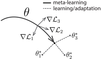
Figure 1. Diagram of our model-agnostic meta-learning algorithm (MAML), which optimizes for a representation θ that can quickly adapt to new tasks.
<details>
<summary>Image 1 Details</summary>
### Visual Description
## Diagram: Meta-Learning Process
### Overview
The image illustrates a meta-learning process, showing the trajectory of meta-learning and the adaptation steps towards task-specific optimal parameters. It depicts how meta-learning guides the model towards a parameter space that allows for efficient adaptation to new tasks.
### Components/Axes
* **θ (Theta)**: Represents the meta-learned parameters. It is shown as a curved solid black line, indicating the trajectory of meta-learning.
* **∇L1, ∇L2, ∇L3**: Gradients of the loss functions for different tasks. These are represented by gray arrows pointing towards the meta-learning trajectory.
* **θ\*1, θ\*2, θ\*3**: Task-specific optimal parameters after adaptation. These are represented by gray dots connected to the meta-learning trajectory by dashed gray lines.
* **Legend (Top-Right)**:
* Solid Black Line: "meta-learning"
* Dashed Gray Line: "learning/adaptation"
### Detailed Analysis
* The solid black line representing "meta-learning" shows a curved path, indicating the optimization process of the meta-learner.
* The gray arrows (∇L1, ∇L2, ∇L3) represent the gradients of the loss functions for different tasks. They point towards the meta-learning trajectory, suggesting that the meta-learner is being guided by these gradients.
* The dashed gray lines represent the adaptation process from the meta-learned parameters (θ) to the task-specific optimal parameters (θ\*1, θ\*2, θ\*3).
* The task-specific optimal parameters (θ\*1, θ\*2, θ\*3) are scattered around the end of the meta-learning trajectory, indicating that the meta-learner has found a parameter space that allows for efficient adaptation to different tasks.
### Key Observations
* The meta-learning trajectory (solid black line) is influenced by the gradients of the loss functions for different tasks (gray arrows).
* The adaptation process (dashed gray lines) leads to task-specific optimal parameters (gray dots).
* The meta-learning process aims to find a parameter space that allows for efficient adaptation to new tasks.
### Interpretation
The diagram illustrates the core concept of meta-learning, where a model learns how to learn. The meta-learner optimizes its parameters (θ) based on the gradients of the loss functions for different tasks (∇L1, ∇L2, ∇L3). This optimization process guides the meta-learner towards a parameter space that allows for efficient adaptation to new tasks, resulting in task-specific optimal parameters (θ\*1, θ\*2, θ\*3). The diagram effectively demonstrates how meta-learning enables a model to quickly adapt to new tasks with minimal training data.
</details>
In our meta-learning scenario, we consider a distribution over tasks p ( T ) that we want our model to be able to adapt to. In the K -shot learning setting, the model is trained to learn a new task T i drawn from p ( T ) from only K samples drawn from q i and feedback L T i generated by T i . During meta-training, a task T i is sampled from p ( T ) , the model is trained with K samples and feedback from the corresponding loss L T i from T i , and then tested on new samples from T i . The model f is then improved by considering how the test error on new data from q i changes with respect to the parameters. In effect, the test error on sampled tasks T i serves as the training error of the meta-learning process. At the end of meta-training, new tasks are sampled from p ( T ) , and meta-performance is measured by the model's performance after learning from K samples. Generally, tasks used for meta-testing are held out during meta-training.
## 2.2. A Model-Agnostic Meta-Learning Algorithm
In contrast to prior work, which has sought to train recurrent neural networks that ingest entire datasets (Santoro et al., 2016; Duan et al., 2016b) or feature embeddings that can be combined with nonparametric methods at test time (Vinyals et al., 2016; Koch, 2015), we propose a method that can learn the parameters of any standard model via meta-learning in such a way as to prepare that model for fast adaptation. The intuition behind this approach is that some internal representations are more transferrable than others. For example, a neural network might learn internal features that are broadly applicable to all tasks in p ( T ) , rather than a single individual task. How can we encourage the emergence of such general-purpose representations? We take an explicit approach to this problem: since the model will be fine-tuned using a gradient-based learning rule on a new task, we will aim to learn a model in such a way that this gradient-based learning rule can make rapid progress on new tasks drawn from p ( T ) , without overfitting. In effect, we will aim to find model parameters that are sensitive to changes in the task, such that small changes in the parameters will produce large improvements on the loss function of any task drawn from p ( T ) , when altered in the direction of the gradient of that loss (see Figure 1). We
| Algorithm 1 Model-Agnostic Meta-Learning | Algorithm 1 Model-Agnostic Meta-Learning |
|--------------------------------------------|-------------------------------------------------------------------------------------|
| Require: p ( T ) : distribution over tasks | Require: p ( T ) : distribution over tasks |
| 1: | randomly initialize θ |
| 2: | while not done do |
| 3: | Sample batch of tasks T i ∼ p ( T ) |
| 4: | for all T i do |
| 5: | Evaluate ∇ θ L T i ( f θ ) with respect to K examples |
| 6: | Compute adapted parameters with gradient de- scent: θ ′ i = θ - α ∇ θ L T i ( f θ ) |
| 7: | end for |
| 8: | Update θ ← θ - β ∇ θ ∑ T i ∼ p ( T ) L T i ( f θ ′ i ) |
| 9: | end while |
make no assumption on the form of the model, other than to assume that it is parametrized by some parameter vector θ , and that the loss function is smooth enough in θ that we can use gradient-based learning techniques.
Formally, we consider a model represented by a parametrized function f θ with parameters θ . When adapting to a new task T i , the model's parameters θ become θ ′ i . In our method, the updated parameter vector θ ′ i is computed using one or more gradient descent updates on task T i . For example, when using one gradient update,
$$\theta _ { i } ^ { \prime } = \theta - \alpha \nabla _ { \theta } \mathcal { L } _ { \mathcal { T } _ { i } } ( f _ { \theta } ) .$$
The step size α may be fixed as a hyperparameter or metalearned. For simplicity of notation, we will consider one gradient update for the rest of this section, but using multiple gradient updates is a straightforward extension.
The model parameters are trained by optimizing for the performance of f θ ′ i with respect to θ across tasks sampled from p ( T ) . More concretely, the meta-objective is as follows:
$$\min _ { \theta } \sum _ { \mathcal { T } _ { i } \sim p ( \mathcal { T } ) } \mathcal { L } _ { \mathcal { T } _ { i } } ( f _ { \theta ^ { \prime } _ { i } } ) = \sum _ { \mathcal { T } _ { i } \sim p ( \mathcal { T } ) } \mathcal { L } _ { \mathcal { T } _ { i } } ( f _ { \theta - \alpha \nabla _ { \theta } \mathcal { L } _ { \mathcal { T } _ { i } } ( f _ { \theta } ) } )$$
Note that the meta-optimization is performed over the model parameters θ , whereas the objective is computed using the updated model parameters θ ′ . In effect, our proposed method aims to optimize the model parameters such that one or a small number of gradient steps on a new task will produce maximally effective behavior on that task.
The meta-optimization across tasks is performed via stochastic gradient descent (SGD), such that the model parameters θ are updated as follows:
$$\theta \leftarrow \theta - \beta \nabla _ { \theta } \sum _ { \mathcal { T } _ { i } \sim p ( \mathcal { T } ) } \mathcal { L } _ { \mathcal { T } _ { i } } ( f _ { \theta ^ { \prime } _ { i } } ) \quad & ( 1 ) \\$$
where β is the meta step size. The full algorithm, in the general case, is outlined in Algorithm 1.
The MAML meta-gradient update involves a gradient through a gradient. Computationally, this requires an additional backward pass through f to compute Hessian-vector products, which is supported by standard deep learning libraries such as TensorFlow (Abadi et al., 2016). In our experiments, we also include a comparison to dropping this backward pass and using a first-order approximation, which we discuss in Section 5.2.
## 3. Species of MAML
In this section, we discuss specific instantiations of our meta-learning algorithm for supervised learning and reinforcement learning. The domains differ in the form of loss function and in how data is generated by the task and presented to the model, but the same basic adaptation mechanism can be applied in both cases.
## 3.1. Supervised Regression and Classification
Few-shot learning is well-studied in the domain of supervised tasks, where the goal is to learn a new function from only a few input/output pairs for that task, using prior data from similar tasks for meta-learning. For example, the goal might be to classify images of a Segway after seeing only one or a few examples of a Segway, with a model that has previously seen many other types of objects. Likewise, in few-shot regression, the goal is to predict the outputs of a continuous-valued function from only a few datapoints sampled from that function, after training on many functions with similar statistical properties.
To formalize the supervised regression and classification problems in the context of the meta-learning definitions in Section 2.1, we can define the horizon H = 1 and drop the timestep subscript on x t , since the model accepts a single input and produces a single output, rather than a sequence of inputs and outputs. The task T i generates K i.i.d. observations x from q i , and the task loss is represented by the error between the model's output for x and the corresponding target values y for that observation and task.
Two common loss functions used for supervised classification and regression are cross-entropy and mean-squared error (MSE), which we will describe below; though, other supervised loss functions may be used as well. For regression tasks using mean-squared error, the loss takes the form:
$$\mathcal { L } _ { \mathcal { T } _ { i } } ( f _ { \phi } ) = \sum _ { x ^ { ( j ) } , y ^ { ( j ) } \sim \mathcal { T } _ { i } } \| f _ { \phi } ( x ^ { ( j ) } ) - y ^ { ( j ) } \| _ { 2 } ^ { 2 } , \quad ( 2 )$$
where x ( j ) , y ( j ) are an input/output pair sampled from task T i . In K -shot regression tasks, K input/output pairs are provided for learning for each task.
Similarly, for discrete classification tasks with a crossentropy loss, the loss takes the form:
$$\mathcal { L } _ { \mathcal { T } _ { i } } ( f _ { \phi } ) = \sum _ { x ^ { ( j ) } , y ^ { ( j ) } \sim \mathcal { T } _ { i } } y ^ { ( j ) } \log f _ { \phi } ( x ^ { ( j ) } ) \\
<text><loc_36><loc_0><loc_500><loc_499>or + (1 - y ^ { ( j ) } ) log(1 - f$_{φ}$ ( x ^ { ( j ) } )) (3) L$_{T}$$_{i}$ = ∑ y (j) log f$_{φ}$(x^{(j)} ) (3) x ^{(j)} ,y^{(j)}∼T$_{i}$ + (1 - y ^{(j)} ) log(1 - f$_{φ}$(x^{(j)})</text>$$
## Algorithm 2 MAMLfor Few-Shot Supervised Learning
Require:
p ( T ) : distribution over tasks
Require:
α , β : step size hyperparameters
- 1: randomly initialize θ
- 2: while not done do
- 3: Sample batch of tasks T i ∼ p ( T )
- 4: for all T i do
- 5: Sample K datapoints D = { x ( j ) , y ( j ) } from T i
- 6: Evaluate ∇ θ L T i ( f θ ) using D and L T i in Equation (2) or (3)
- 7: Compute adapted parameters with gradient descent: θ ′ i = θ - α ∇ θ L T i ( f θ )
- 8: Sample datapoints D ′ i = { x ( j ) , y ( j ) } from T i for the meta-update
- 9: end for
- 10: Update θ ← θ - β ∇ θ ∑ T i ∼ p ( T ) L T i ( f θ ′ i ) using each D ′ i and L T i in Equation 2 or 3
- 11: end while
According to the conventional terminology, K -shot classification tasks use K input/output pairs from each class, for a total of NK data points for N -way classification. Given a distribution over tasks p ( T i ) , these loss functions can be directly inserted into the equations in Section 2.2 to perform meta-learning, as detailed in Algorithm 2.
## 3.2. Reinforcement Learning
In reinforcement learning (RL), the goal of few-shot metalearning is to enable an agent to quickly acquire a policy for a new test task using only a small amount of experience in the test setting. A new task might involve achieving a new goal or succeeding on a previously trained goal in a new environment. For example, an agent might learn to quickly figure out how to navigate mazes so that, when faced with a new maze, it can determine how to reliably reach the exit with only a few samples. In this section, we will discuss how MAML can be applied to meta-learning for RL.
Each RL task T i contains an initial state distribution q i ( x 1 ) and a transition distribution q i ( x t +1 | x t , a t ) , and the loss L T i corresponds to the (negative) reward function R . The entire task is therefore a Markov decision process (MDP) with horizon H , where the learner is allowed to query a limited number of sample trajectories for few-shot learning. Any aspect of the MDP may change across tasks in p ( T ) . The model being learned, f θ , is a policy that maps from states x t to a distribution over actions a t at each timestep t ∈ { 1 , ..., H } . The loss for task T i and model f φ takes the form
$$\mathcal { L } _ { \mathcal { T } _ { i } } ( f _ { \phi } ) = - \mathbb { E } _ { x _ { t } , a _ { t } \sim f _ { \phi } , q _ { \mathcal { T } _ { i } } } \left [ \sum _ { t = 1 } ^ { H } R _ { i } ( x _ { t } , a _ { t } ) \right ] .
</doctag>$$
In K -shot reinforcement learning, K rollouts from f θ and task T i , ( x 1 , a 1 , ... x H ) , and the corresponding rewards R ( x t , a t ) , may be used for adaptation on a new task T i .
## Algorithm 3 MAMLfor Reinforcement Learning
Require:
p ( T ) : distribution over tasks
Require:
α , β : step size hyperparameters
- 1: randomly initialize θ
- 2: while not done do
- 3: Sample batch of tasks T i ∼ p ( T )
- 4: for all T i do
- 5: Sample K trajectories D = { ( x 1 , a 1 , ... x H ) } using f θ in T i
- 6: Evaluate ∇ θ L T i ( f θ ) using D and L T i in Equation 4
- 7: Compute adapted parameters with gradient descent: θ ′ i = θ -α ∇ θ L T i ( f θ )
- 8: Sample trajectories D ′ i = { ( x 1 , a 1 , ... x H ) } using f θ ′ i in T i
- 9: end for
- 10: Update θ ← θ -β ∇ θ ∑ T i ∼ p ( T ) L T i ( f θ ′ i ) using each D ′ i and L T i in Equation 4
- 11: end while
Since the expected reward is generally not differentiable due to unknown dynamics, we use policy gradient methods to estimate the gradient both for the model gradient update(s) and the meta-optimization. Since policy gradients are an on-policy algorithm, each additional gradient step during the adaptation of f θ requires new samples from the current policy f θ i ′ . We detail the algorithm in Algorithm 3. This algorithm has the same structure as Algorithm 2, with the principal difference being that steps 5 and 8 require sampling trajectories from the environment corresponding to task T i . Practical implementations of this method may also use a variety of improvements recently proposed for policy gradient algorithms, including state or action-dependent baselines and trust regions (Schulman et al., 2015).
## 4. Related Work
The method that we propose in this paper addresses the general problem of meta-learning (Thrun & Pratt, 1998; Schmidhuber, 1987; Naik & Mammone, 1992), which includes few-shot learning. A popular approach for metalearning is to train a meta-learner that learns how to update the parameters of the learner's model (Bengio et al., 1992; Schmidhuber, 1992; Bengio et al., 1990). This approach has been applied to learning to optimize deep networks (Hochreiter et al., 2001; Andrychowicz et al., 2016; Li & Malik, 2017), as well as for learning dynamically changing recurrent networks (Ha et al., 2017). One recent approach learns both the weight initialization and the optimizer, for few-shot image recognition (Ravi & Larochelle, 2017). Unlike these methods, the MAML learner's weights are updated using the gradient, rather than a learned update; our method does not introduce additional parameters for meta-learning nor require a particular learner architecture.
Few-shot learning methods have also been developed for
specific tasks such as generative modeling (Edwards & Storkey, 2017; Rezende et al., 2016) and image recognition (Vinyals et al., 2016). One successful approach for few-shot classification is to learn to compare new examples in a learned metric space using e.g. Siamese networks (Koch, 2015) or recurrence with attention mechanisms (Vinyals et al., 2016; Shyam et al., 2017; Snell et al., 2017). These approaches have generated some of the most successful results, but are difficult to directly extend to other problems, such as reinforcement learning. Our method, in contrast, is agnostic to the form of the model and to the particular learning task.
Another approach to meta-learning is to train memoryaugmented models on many tasks, where the recurrent learner is trained to adapt to new tasks as it is rolled out. Such networks have been applied to few-shot image recognition (Santoro et al., 2016; Munkhdalai & Yu, 2017) and learning 'fast' reinforcement learning agents (Duan et al., 2016b; Wang et al., 2016). Our experiments show that our method outperforms the recurrent approach on fewshot classification. Furthermore, unlike these methods, our approach simply provides a good weight initialization and uses the same gradient descent update for both the learner and meta-update. As a result, it is straightforward to finetune the learner for additional gradient steps.
Our approach is also related to methods for initialization of deep networks. In computer vision, models pretrained on large-scale image classification have been shown to learn effective features for a range of problems (Donahue et al., 2014). In contrast, our method explicitly optimizes the model for fast adaptability, allowing it to adapt to new tasks with only a few examples. Our method can also be viewed as explicitly maximizing sensitivity of new task losses to the model parameters. A number of prior works have explored sensitivity in deep networks, often in the context of initialization (Saxe et al., 2014; Kirkpatrick et al., 2016). Most of these works have considered good random initializations, though a number of papers have addressed datadependent initializers (Kr¨ ahenb¨ uhl et al., 2016; Salimans & Kingma, 2016), including learned initializations (Husken & Goerick, 2000; Maclaurin et al., 2015). In contrast, our method explicitly trains the parameters for sensitivity on a given task distribution, allowing for extremely efficient adaptation for problems such as K -shot learning and rapid reinforcement learning in only one or a few gradient steps.
## 5. Experimental Evaluation
The goal of our experimental evaluation is to answer the following questions: (1) Can MAML enable fast learning of new tasks? (2) Can MAML be used for meta-learning in multiple different domains, including supervised regression, classification, and reinforcement learning? (3) Can a model learned with MAML continue to improve with additional gradient updates and/or examples?
All of the meta-learning problems that we consider require some amount of adaptation to new tasks at test-time. When possible, we compare our results to an oracle that receives the identity of the task (which is a problem-dependent representation) as an additional input, as an upper bound on the performance of the model. All of the experiments were performed using TensorFlow (Abadi et al., 2016), which allows for automatic differentiation through the gradient update(s) during meta-learning. The code is available online 1 .
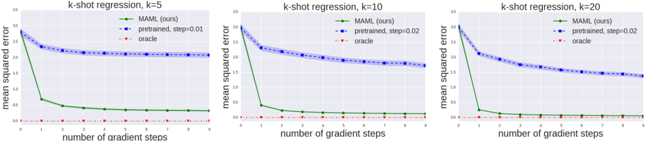
## 5.1. Regression
We start with a simple regression problem that illustrates the basic principles of MAML. Each task involves regressing from the input to the output of a sine wave, where the amplitude and phase of the sinusoid are varied between tasks. Thus, p ( T ) is continuous, where the amplitude varies within [0 . 1 , 5 . 0] and the phase varies within [0 , π ] , and the input and output both have a dimensionality of 1 . During training and testing, datapoints x are sampled uniformly from [ -5 . 0 , 5 . 0] . The loss is the mean-squared error between the prediction f ( x ) and true value. The regressor is a neural network model with 2 hidden layers of size 40 with ReLU nonlinearities. When training with MAML, we use one gradient update with K = 10 examples with a fixed step size α = 0 . 01 , and use Adam as the metaoptimizer (Kingma & Ba, 2015). The baselines are likewise trained with Adam. To evaluate performance, we finetune a single meta-learned model on varying numbers of K examples, and compare performance to two baselines: (a) pretraining on all of the tasks, which entails training a network to regress to random sinusoid functions and then, at test-time, fine-tuning with gradient descent on the K provided points, using an automatically tuned step size, and (b) an oracle which receives the true amplitude and phase as input. In Appendix C, we show comparisons to additional multi-task and adaptation methods.
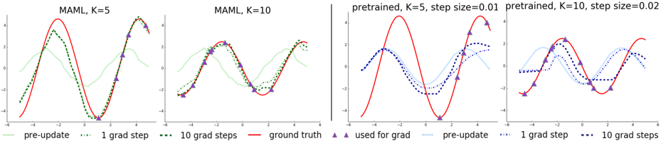
We evaluate performance by fine-tuning the model learned by MAML and the pretrained model on K = { 5 , 10 , 20 } datapoints. During fine-tuning, each gradient step is computed using the same K datapoints. The qualitative results, shown in Figure 2 and further expanded on in Appendix B show that the learned model is able to quickly adapt with only 5 datapoints, shown as purple triangles, whereas the model that is pretrained using standard supervised learning on all tasks is unable to adequately adapt with so few datapoints without catastrophic overfitting. Crucially, when the K datapoints are all in one half of the input range, the
1 Code for the regression and supervised experiments is at github.com/cbfinn/maml and code for the RL experiments is at github.com/cbfinn/maml\_rl
Figure 2. Few-shot adaptation for the simple regression task. Left: Note that MAML is able to estimate parts of the curve where there are no datapoints, indicating that the model has learned about the periodic structure of sine waves. Right: Fine-tuning of a model pretrained on the same distribution of tasks without MAML, with a tuned step size. Due to the often contradictory outputs on the pre-training tasks, this model is unable to recover a suitable representation and fails to extrapolate from the small number of test-time samples.
<details>
<summary>Image 2 Details</summary>
### Visual Description
## Chart: Comparison of MAML and Pretrained Models
### Overview
The image presents four line charts comparing the performance of MAML (Model-Agnostic Meta-Learning) and pretrained models with different configurations. Each chart displays the "ground truth" function (red line) along with the model's predictions after different numbers of gradient steps. The charts vary in the number of inner loop updates (K) and step size.
### Components/Axes
Each chart has the following components:
* **Title:** Specifies the model type (MAML or pretrained) and parameters (K value, step size).
* **X-axis:** Ranges from approximately -6 to 6. No explicit label is provided, but it likely represents the input to the function.
* **Y-axis:** Ranges from -4 to 4. No explicit label is provided, but it likely represents the output of the function.
* **Ground Truth:** Represented by a solid red line.
* **Pre-update:** Represented by a light green dotted line (MAML) or light blue dotted line (pretrained).
* **1 grad step:** Represented by a dark green dotted line (MAML) or dark blue dotted line (pretrained).
* **10 grad steps:** Represented by a dark green dashed line (MAML) or dark blue dashed line (pretrained).
* **Used for grad:** Represented by purple triangles.
The legend is located at the bottom of the image and applies to all four charts.
### Detailed Analysis
**Chart 1: MAML, K=5**
* **Ground Truth (red):** A sinusoidal curve oscillating between approximately -4 and 4.
* **Pre-update (light green dotted):** Starts around y=0 at x=-6, rises to a peak around y=2 at x=-3, then decreases to a trough around y=-1 at x=0, and rises again.
* **1 grad step (dark green dotted):** Starts around y=-3 at x=-6, rises to a peak around y=3 at x=-3, then decreases to a trough around y=-4 at x=0, and rises again.
* **10 grad steps (dark green dashed):** Closely follows the ground truth, indicating good adaptation.
* **Used for grad (purple triangles):** Located on the ground truth curve.
**Chart 2: MAML, K=10**
* **Ground Truth (red):** Similar sinusoidal curve as in Chart 1.
* **Pre-update (light green dotted):** Starts around y=0 at x=-6, rises to a peak around y=2 at x=-3, then decreases to a trough around y=-1 at x=0, and rises again.
* **1 grad step (dark green dotted):** Starts around y=-3 at x=-6, rises to a peak around y=3 at x=-3, then decreases to a trough around y=-4 at x=0, and rises again.
* **10 grad steps (dark green dashed):** Closely follows the ground truth, indicating good adaptation.
* **Used for grad (purple triangles):** Located on the ground truth curve.
**Chart 3: pretrained, K=5, step size=0.01**
* **Ground Truth (red):** Similar sinusoidal curve as in Chart 1.
* **Pre-update (light blue dotted):** Starts around y=0 at x=-6, rises to a peak around y=2 at x=-3, then decreases to a trough around y=-1 at x=0, and rises again.
* **1 grad step (dark blue dotted):** Starts around y=-1 at x=-6, rises to a peak around y=2 at x=-3, then decreases to a trough around y=-2 at x=0, and rises again.
* **10 grad steps (dark blue dashed):** Starts around y=-2 at x=-6, rises to a peak around y=3 at x=-3, then decreases to a trough around y=-3 at x=0, and rises again.
* **Used for grad (purple triangles):** Located on the ground truth curve.
**Chart 4: pretrained, K=10, step size=0.02**
* **Ground Truth (red):** Similar sinusoidal curve as in Chart 1.
* **Pre-update (light blue dotted):** Starts around y=0 at x=-6, rises to a peak around y=2 at x=-3, then decreases to a trough around y=-1 at x=0, and rises again.
* **1 grad step (dark blue dotted):** Starts around y=-1 at x=-6, rises to a peak around y=2 at x=-3, then decreases to a trough around y=-2 at x=0, and rises again.
* **10 grad steps (dark blue dashed):** Starts around y=-2 at x=-6, rises to a peak around y=3 at x=-3, then decreases to a trough around y=-3 at x=0, and rises again.
* **Used for grad (purple triangles):** Located on the ground truth curve.
### Key Observations
* In both MAML charts (K=5 and K=10), the "10 grad steps" line closely aligns with the "ground truth" line, indicating effective adaptation to the target function.
* In the pretrained charts, the "10 grad steps" line does not align as closely with the "ground truth" line as in the MAML charts, suggesting that MAML adapts more effectively with fewer updates.
* The "pre-update" lines show the initial state of the model before any adaptation.
* The purple triangles ("used for grad") mark the data points used for gradient calculation.
### Interpretation
The charts demonstrate the effectiveness of MAML in adapting to new tasks with a small number of gradient updates. The MAML models, with both K=5 and K=10, quickly converge to the "ground truth" function after just 10 gradient steps. In contrast, the pretrained models, even with different step sizes, do not adapt as effectively, suggesting that MAML is better suited for few-shot learning scenarios where rapid adaptation is crucial. The "pre-update" lines highlight the importance of a good initialization, while the "used for grad" markers indicate the data points that drive the adaptation process. The choice of K and step size influences the adaptation process, but MAML appears to be more robust in this comparison.
</details>
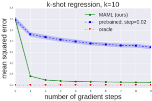
Figure 3. Quantitative sinusoid regression results showing the learning curve at meta test-time. Note that MAML continues to improve with additional gradient steps without overfitting to the extremely small dataset during meta-testing, achieving a loss that is substantially lower than the baseline fine-tuning approach.
<details>
<summary>Image 3 Details</summary>
### Visual Description
## Chart: K-shot Regression Performance
### Overview
The image is a line chart comparing the performance of three different regression models: MAML (ours), a pretrained model, and an oracle model. The chart plots the mean squared error against the number of gradient steps.
### Components/Axes
* **Title:** k-shot regression, k=10
* **X-axis:** number of gradient steps (values from 0 to 9)
* **Y-axis:** mean squared error (values from 0.0 to 3.5)
* **Legend:**
* **Green line with circle markers:** MAML (ours)
* **Blue dashed line with square markers:** pretrained, step=0.02
* **Red dotted line with triangle markers:** oracle
### Detailed Analysis
* **MAML (ours) - Green Line:** The green line starts at approximately 3.0 and rapidly decreases to around 0.4 at step 1. It then continues to decrease gradually, reaching a value of approximately 0.1 at step 9.
* Step 0: ~3.0
* Step 1: ~0.4
* Step 2: ~0.25
* Step 3: ~0.2
* Step 4: ~0.17
* Step 5: ~0.15
* Step 6: ~0.14
* Step 7: ~0.13
* Step 8: ~0.12
* Step 9: ~0.11
* **Pretrained, step=0.02 - Blue Line:** The blue dashed line starts at approximately 3.0 and gradually decreases over the gradient steps. There is a shaded blue area around the line, indicating the uncertainty or variance.
* Step 0: ~3.0
* Step 1: ~2.3
* Step 2: ~2.1
* Step 3: ~2.05
* Step 4: ~1.95
* Step 5: ~1.9
* Step 6: ~1.85
* Step 7: ~1.8
* Step 8: ~1.78
* Step 9: ~1.7
* **Oracle - Red Line:** The red dotted line remains close to 0.0 throughout all gradient steps.
* Step 0: ~0.05
* Step 1: ~0.02
* Step 2: ~0.01
* Step 3: ~0.01
* Step 4: ~0.01
* Step 5: ~0.01
* Step 6: ~0.01
* Step 7: ~0.01
* Step 8: ~0.01
* Step 9: ~0.01
### Key Observations
* The MAML model shows a significant initial drop in mean squared error, indicating rapid learning.
* The pretrained model decreases more slowly than the MAML model.
* The oracle model consistently has the lowest mean squared error, representing the ideal performance.
### Interpretation
The chart demonstrates that the MAML model (ours) achieves a lower mean squared error compared to the pretrained model, especially in the initial gradient steps. The oracle model serves as a benchmark, showing the lowest possible error. The MAML model's rapid initial learning suggests it is more effective at adapting to the task compared to the pretrained model. The shaded area around the "pretrained" line indicates the variance in the model's performance. The oracle model's consistently low error indicates it has perfect knowledge of the task.
</details>
model trained with MAML can still infer the amplitude and phase in the other half of the range, demonstrating that the MAML trained model f has learned to model the periodic nature of the sine wave. Furthermore, we observe both in the qualitative and quantitative results (Figure 3 and Appendix B) that the model learned with MAML continues to improve with additional gradient steps, despite being trained for maximal performance after one gradient step. This improvement suggests that MAML optimizes the parameters such that they lie in a region that is amenable to fast adaptation and is sensitive to loss functions from p ( T ) , as discussed in Section 2.2, rather than overfitting to parameters θ that only improve after one step.
## 5.2. Classification
To evaluate MAML in comparison to prior meta-learning and few-shot learning algorithms, we applied our method to few-shot image recognition on the Omniglot (Lake et al., 2011) and MiniImagenet datasets. The Omniglot dataset consists of 20 instances of 1623 characters from 50 different alphabets. Each instance was drawn by a different person. The MiniImagenet dataset was proposed by Ravi & Larochelle (2017), and involves 64 training classes, 12 validation classes, and 24 test classes. The Omniglot and MiniImagenet image recognition tasks are the most common recently used few-shot learning benchmarks (Vinyals et al., 2016; Santoro et al., 2016; Ravi & Larochelle, 2017).
We follow the experimental protocol proposed by Vinyals et al. (2016), which involves fast learning of N -way classification with 1 or 5 shots. The problem of N -way classification is set up as follows: select N unseen classes, provide the model with K different instances of each of the N classes, and evaluate the model's ability to classify new instances within the N classes. For Omniglot, we randomly select 1200 characters for training, irrespective of alphabet, and use the remaining for testing. The Omniglot dataset is augmented with rotations by multiples of 90 degrees, as proposed by Santoro et al. (2016).
Our model follows the same architecture as the embedding function used by Vinyals et al. (2016), which has 4 modules with a 3 × 3 convolutions and 64 filters, followed by batch normalization (Ioffe & Szegedy, 2015), a ReLU nonlinearity, and 2 × 2 max-pooling. The Omniglot images are downsampled to 28 × 28 , so the dimensionality of the last hidden layer is 64 . As in the baseline classifier used by Vinyals et al. (2016), the last layer is fed into a softmax. For Omniglot, we used strided convolutions instead of max-pooling. For MiniImagenet, we used 32 filters per layer to reduce overfitting, as done by (Ravi & Larochelle, 2017). In order to also provide a fair comparison against memory-augmented neural networks (Santoro et al., 2016) and to test the flexibility of MAML, we also provide results for a non-convolutional network. For this, we use a network with 4 hidden layers with sizes 256 , 128 , 64 , 64 , each including batch normalization and ReLU nonlinearities, followed by a linear layer and softmax. For all models, the loss function is the cross-entropy error between the predicted and true class. Additional hyperparameter details are included in Appendix A.1.
We present the results in Table 1. The convolutional model learned by MAML compares well to the state-of-the-art results on this task, narrowly outperforming the prior methods. Some of these existing methods, such as matching networks, Siamese networks, and memory models are designed with few-shot classification in mind, and are not readily applicable to domains such as reinforcement learning. Additionally, the model learned with MAML uses
Table 1. Few-shot classification on held-out Omniglot characters (top) and the MiniImagenet test set (bottom). MAML achieves results that are comparable to or outperform state-of-the-art convolutional and recurrent models. Siamese nets, matching nets, and the memory module approaches are all specific to classification, and are not directly applicable to regression or RL scenarios. The ± shows 95% confidence intervals over tasks. Note that the Omniglot results may not be strictly comparable since the train/test splits used in the prior work were not available. The MiniImagenet evaluation of baseline methods and matching networks is from Ravi & Larochelle (2017).
| | 5-way Accuracy | 5-way Accuracy | 20-way Accuracy | 20-way Accuracy |
|----------------------------------------------|------------------|------------------|-------------------|-------------------|
| Omniglot (Lake et al., 2011) | 1-shot | 5-shot | 1-shot | 5-shot |
| MANN, no conv (Santoro et al., 2016) | 82 . 8% | 94 . 9% | - | - |
| MAML, no conv (ours) | 89 . 7 ± 1 . 1 % | 97 . 5 ± 0 . 6 % | - | - |
| Siamese nets (Koch, 2015) | 97 . 3% | 98 . 4% | 88 . 2% | 97 . 0% |
| matching nets (Vinyals et al., 2016) | 98 . 1% | 98 . 9% | 93 . 8% | 98 . 5% |
| neural statistician (Edwards &Storkey, 2017) | 98 . 1% | 99 . 5% | 93 . 2% | 98 . 1% |
| memory mod. (Kaiser et al., 2017) | 98 . 4% | 99 . 6% | 95 . 0% | 98 . 6% |
| MAML(ours) | 98 . 7 ± 0 . 4 % | 99 . 9 ± 0 . 1 % | 95 . 8 ± 0 . 3 % | 98 . 9 ± 0 . 2 % |
| | 5-way Accuracy | 5-way Accuracy |
|--------------------------------------------|--------------------|--------------------|
| MiniImagenet (Ravi &Larochelle, 2017) | 1-shot | 5-shot |
| fine-tuning baseline | 28 . 86 ± 0 . 54% | 49 . 79 ± 0 . 79% |
| nearest neighbor baseline | 41 . 08 ± 0 . 70% | 51 . 04 ± 0 . 65% |
| matching nets (Vinyals et al., 2016) | 43 . 56 ± 0 . 84% | 55 . 31 ± 0 . 73% |
| meta-learner LSTM (Ravi &Larochelle, 2017) | 43 . 44 ± 0 . 77% | 60 . 60 ± 0 . 71% |
| MAML, first order approx. (ours) | 48 . 07 ± 1 . 75 % | 63 . 15 ± 0 . 91 % |
| MAML(ours) | 48 . 70 ± 1 . 84 % | 63 . 11 ± 0 . 92 % |
fewer overall parameters compared to matching networks and the meta-learner LSTM, since the algorithm does not introduce any additional parameters beyond the weights of the classifier itself. Compared to these prior methods, memory-augmented neural networks (Santoro et al., 2016) specifically, and recurrent meta-learning models in general, represent a more broadly applicable class of methods that, like MAML, can be used for other tasks such as reinforcement learning (Duan et al., 2016b; Wang et al., 2016). However, as shown in the comparison, MAML significantly outperforms memory-augmented networks and the meta-learner LSTM on 5-way Omniglot and MiniImagenet classification, both in the 1 -shot and 5 -shot case.
A significant computational expense in MAML comes from the use of second derivatives when backpropagating the meta-gradient through the gradient operator in the meta-objective (see Equation (1)). On MiniImagenet, we show a comparison to a first-order approximation of MAML, where these second derivatives are omitted. Note that the resulting method still computes the meta-gradient at the post-update parameter values θ ′ i , which provides for effective meta-learning. Surprisingly however, the performance of this method is nearly the same as that obtained with full second derivatives, suggesting that most of the improvement in MAML comes from the gradients of the objective at the post-update parameter values, rather than the second order updates from differentiating through the gradient update. Past work has observed that ReLU neural networks are locally almost linear (Goodfellow et al., 2015), which suggests that second derivatives may be close to zero in most cases, partially explaining the good perfor-
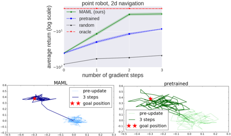
Figure 4. Top: quantitative results from 2D navigation task, Bottom: qualitative comparison between model learned with MAML and with fine-tuning from a pretrained network.
<details>
<summary>Image 4 Details</summary>
### Visual Description
## Chart and Trajectory Plots: Point Robot 2D Navigation
### Overview
The image presents a combination of a line chart and two trajectory plots, all related to the performance of different learning algorithms for a point robot navigating in 2D. The line chart compares the average return (log scale) of four algorithms (MAML, pretrained, random, and oracle) over a number of gradient steps. The trajectory plots visualize the robot's movement during the "MAML" and "pretrained" algorithms, showing the path before and after updates, and indicating the goal position.
### Components/Axes
**Line Chart:**
* **Title:** point robot, 2d navigation
* **X-axis:** number of gradient steps (values: 0, 1, 2, 3)
* **Y-axis:** average return (log scale) (values range from -10<sup>2</sup> to -10<sup>1</sup>)
* **Legend:** Located in the top-right of the chart.
* MAML (ours): Solid green line with shaded region indicating uncertainty.
* pretrained: Dashed blue line with shaded region indicating uncertainty.
* random: Dotted black line.
* oracle: Dashed red line with plus markers.
**Trajectory Plots:**
* **Titles:** MAML (left), pretrained (right)
* **Axes:** Both plots have similar x and y axes, ranging approximately from -0.5 to 0.6.
* **Legend:** Located in the top-right of each plot.
* pre-update: Light blue (MAML) or light green (pretrained) line, showing the initial trajectory.
* 3 steps: Dark blue (MAML) or dark green (pretrained) line, showing the trajectory after 3 gradient steps.
* goal position: Red star marker.
### Detailed Analysis
**Line Chart Data:**
* **MAML (ours):** Solid green line. The average return starts around -10<sup>1</sup> at 0 gradient steps, increases to approximately 5 at 1 step, reaches approximately 30 at 2 steps, and plateaus at approximately 30 at 3 steps.
* **pretrained:** Dashed blue line. The average return starts around -10<sup>1</sup> at 0 gradient steps, increases to approximately 5 at 1 step, reaches approximately 10 at 2 steps, and plateaus at approximately 10 at 3 steps.
* **random:** Dotted black line. The average return remains relatively constant around -10<sup>2</sup> across all gradient steps.
* **oracle:** Dashed red line with plus markers. The average return remains constant at approximately 30 across all gradient steps.
**Trajectory Plots:**
* **MAML:** The "pre-update" trajectory (light blue) shows erratic movement. After 3 steps (dark blue), the trajectory converges towards the goal position (red star).
* **pretrained:** The "pre-update" trajectory (light green) shows erratic movement. After 3 steps (dark green), the trajectory converges towards the goal position (red star).
### Key Observations
* MAML and pretrained algorithms show significant improvement in average return with increasing gradient steps, while the random algorithm remains consistently low.
* The oracle algorithm provides a constant, high average return, serving as a benchmark.
* The trajectory plots indicate that both MAML and pretrained algorithms learn to navigate towards the goal position after a few gradient steps.
### Interpretation
The line chart demonstrates the effectiveness of meta-learning (MAML) and pretraining in improving the performance of a point robot's navigation task. The MAML algorithm appears to outperform the pretrained algorithm, achieving a higher average return after a few gradient steps. The random algorithm's consistently low performance highlights the importance of learning in this task. The oracle algorithm represents an ideal, potentially unattainable, performance level.
The trajectory plots visually confirm the learning process, showing how the robot's movement becomes more directed towards the goal position as the algorithms are updated. The initial erratic movements ("pre-update") are gradually replaced by more focused trajectories after 3 gradient steps.
The data suggests that MAML is a more effective learning algorithm for this specific task compared to pretraining. The comparison against a random strategy and an oracle provides context for the performance gains achieved by MAML and pretraining.
</details>
mance of the first-order approximation. This approximation removes the need for computing Hessian-vector products in an additional backward pass, which we found led to roughly 33% speed-up in network computation.
## 5.3. Reinforcement Learning
To evaluate MAML on reinforcement learning problems, we constructed several sets of tasks based off of the simulated continuous control environments in the rllab benchmark suite (Duan et al., 2016a). We discuss the individual domains below. In all of the domains, the model trained by MAML is a neural network policy with two hidden layers of size 100 , with ReLU nonlinearities. The gradient updates are computed using vanilla policy gradient (REINFORCE) (Williams, 1992), and we use trust-region policy optimization (TRPO) as the meta-optimizer (Schulman et al., 2015). In order to avoid computing third derivatives,
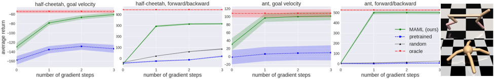
Figure 5. Reinforcement learning results for the half-cheetah and ant locomotion tasks, with the tasks shown on the far right. Each gradient step requires additional samples from the environment, unlike the supervised learning tasks. The results show that MAML can adapt to new goal velocities and directions substantially faster than conventional pretraining or random initialization, achieving good performs in just two or three gradient steps. We exclude the goal velocity, random baseline curves, since the returns are much worse ( < -200 for cheetah and < -25 for ant).
<details>
<summary>Image 5 Details</summary>
### Visual Description
## Chart: Performance Comparison of Different Algorithms on Half-Cheetah and Ant Tasks
### Overview
The image presents four line charts comparing the performance of different algorithms (MAML, pretrained, random, and oracle) on two tasks: "half-cheetah" and "ant." For each task, two metrics are evaluated: "goal velocity" and "forward/backward" movement. The x-axis represents the number of gradient steps, and the y-axis represents the average return. A legend on the right side of the charts identifies the color-coded algorithms. The image also includes a visual representation of the "ant" task.
### Components/Axes
* **X-axis:** Number of gradient steps (0, 1, 2, 3)
* **Y-axis:** Average return (varies depending on the chart)
* **Titles:**
* Top-left: "half-cheetah, goal velocity"
* Top-middle-left: "half-cheetah, forward/backward"
* Top-middle-right: "ant, goal velocity"
* Top-right: "ant, forward/backward"
* **Legend (right side of the charts):**
* Green: MAML (ours)
* Blue: pretrained
* Black: random
* Red: oracle
### Detailed Analysis
**1. Half-Cheetah, Goal Velocity**
* **Y-axis:** Average return ranges from -160 to -60.
* **Oracle (Red):** The line is approximately constant at -60.
* **MAML (Green):** The line slopes upward from approximately -130 at 0 steps to approximately -80 at 1 step, then plateaus around -75 at 2 and 3 steps.
* **Pretrained (Blue):** The line slopes upward from approximately -160 at 0 steps to approximately -135 at 1 step, then plateaus around -130 at 2 and 3 steps.
* **Random (Black):** Not present in this chart.
**2. Half-Cheetah, Forward/Backward**
* **Y-axis:** Ranges from 0 to 400.
* **Oracle (Red):** The line is approximately constant at 400.
* **MAML (Green):** The line slopes upward from approximately 0 at 0 steps to approximately 300 at 1 step, then plateaus around 320 at 2 and 3 steps.
* **Pretrained (Blue):** The line slopes upward from approximately 0 at 0 steps to approximately 50 at 3 steps.
* **Random (Black):** The line slopes upward from approximately 0 at 0 steps to approximately 100 at 3 steps.
**3. Ant, Goal Velocity**
* **Y-axis:** Ranges from -20 to 120.
* **Oracle (Red):** The line is approximately constant at 115.
* **MAML (Green):** The line slopes upward from approximately 0 at 0 steps to approximately 95 at 1 step, then plateaus around 100 at 2 and 3 steps.
* **Pretrained (Blue):** The line slopes upward from approximately -20 at 0 steps to approximately 10 at 1 step, then plateaus around 15 at 2 and 3 steps.
* **Random (Black):** Not present in this chart.
**4. Ant, Forward/Backward**
* **Y-axis:** Ranges from 0 to 500.
* **Oracle (Red):** The line is approximately constant at 520.
* **MAML (Green):** The line slopes upward from approximately 0 at 0 steps to approximately 500 at 1 step, then plateaus around 500 at 2 and 3 steps.
* **Pretrained (Blue):** The line is approximately constant at 0.
* **Random (Black):** Not present in this chart.
### Key Observations
* The "oracle" algorithm consistently achieves the highest average return across all tasks and metrics.
* The "MAML" algorithm generally outperforms the "pretrained" and "random" algorithms, especially after a few gradient steps.
* The "pretrained" algorithm shows some improvement over the "random" algorithm in the "half-cheetah" tasks, but its performance is significantly lower than "MAML" and "oracle."
* The performance of all algorithms tends to plateau after 1 or 2 gradient steps.
### Interpretation
The charts demonstrate the effectiveness of the MAML algorithm in adapting to new tasks with a small number of gradient steps. The "oracle" algorithm represents an ideal performance ceiling, while the "pretrained" and "random" algorithms serve as baselines. The results suggest that MAML can quickly learn and achieve near-optimal performance, making it a promising approach for meta-learning and few-shot learning scenarios. The plateauing of performance after a few gradient steps indicates that further optimization may not yield significant improvements.
</details>
we use finite differences to compute the Hessian-vector products for TRPO. For both learning and meta-learning updates, we use the standard linear feature baseline proposed by Duan et al. (2016a), which is fitted separately at each iteration for each sampled task in the batch. We compare to three baseline models: (a) pretraining one policy on all of the tasks and then fine-tuning, (b) training a policy from randomly initialized weights, and (c) an oracle policy which receives the parameters of the task as input, which for the tasks below corresponds to a goal position, goal direction, or goal velocity for the agent. The baseline models of (a) and (b) are fine-tuned with gradient descent with a manually tuned step size. Videos of the learned policies can be viewed at sites.google.com/view/maml
2D Navigation. In our first meta-RL experiment, we study a set of tasks where a point agent must move to different goal positions in 2D, randomly chosen for each task within a unit square. The observation is the current 2D position, and actions correspond to velocity commands clipped to be in the range [ -0 . 1 , 0 . 1] . The reward is the negative squared distance to the goal, and episodes terminate when the agent is within 0 . 01 of the goal or at the horizon of H = 100 . The policy was trained with MAML to maximize performance after 1 policy gradient update using 20 trajectories. Additional hyperparameter settings for this problem and the following RL problems are in Appendix A.2. In our evaluation, we compare adaptation to a new task with up to 4 gradient updates, each with 40 samples. The results in Figure 4 show the adaptation performance of models that are initialized with MAML, conventional pretraining on the same set of tasks, random initialization, and an oracle policy that receives the goal position as input. The results show that MAML can learn a model that adapts much more quickly in a single gradient update, and furthermore continues to improve with additional updates.
Locomotion. To study how well MAML can scale to more complex deep RL problems, we also study adaptation on high-dimensional locomotion tasks with the MuJoCo simulator (Todorov et al., 2012). The tasks require two simulated robots - a planar cheetah and a 3D quadruped (the 'ant') - to run in a particular direction or at a particular velocity. In the goal velocity experiments, the reward is the negative absolute value between the current velocity of the agent and a goal, which is chosen uniformly at random between 0 . 0 and 2 . 0 for the cheetah and between 0 . 0 and 3 . 0 for the ant. In the goal direction experiments, the reward is the magnitude of the velocity in either the forward or backward direction, chosen at random for each task in p ( T ) . The horizon is H = 200 , with 20 rollouts per gradient step for all problems except the ant forward/backward task, which used 40 rollouts per step. The results in Figure 5 show that MAML learns a model that can quickly adapt its velocity and direction with even just a single gradient update, and continues to improve with more gradient steps. The results also show that, on these challenging tasks, the MAML initialization substantially outperforms random initialization and pretraining. In fact, pretraining is in some cases worse than random initialization, a fact observed in prior RL work (Parisotto et al., 2016).
## 6. Discussion and Future Work
We introduced a meta-learning method based on learning easily adaptable model parameters through gradient descent. Our approach has a number of benefits. It is simple and does not introduce any learned parameters for metalearning. It can be combined with any model representation that is amenable to gradient-based training, and any differentiable objective, including classification, regression, and reinforcement learning. Lastly, since our method merely produces a weight initialization, adaptation can be performed with any amount of data and any number of gradient steps, though we demonstrate state-of-the-art results on classification with only one or five examples per class. We also show that our method can adapt an RL agent using policy gradients and a very modest amount of experience.
Reusing knowledge from past tasks may be a crucial ingredient in making high-capacity scalable models, such as deep neural networks, amenable to fast training with small datasets. We believe that this work is one step toward a simple and general-purpose meta-learning technique that can be applied to any problem and any model. Further research in this area can make multitask initialization a standard ingredient in deep learning and reinforcement learning.
## Acknowledgements
The authors would like to thank Xi Chen and Trevor Darrell for helpful discussions, Yan Duan and Alex Lee for technical advice, Nikhil Mishra, Haoran Tang, and Greg Kahn for feedback on an early draft of the paper, and the anonymous reviewers for their comments. This work was supported in part by an ONR PECASE award and an NSF GRFP award.
## References
- Abadi, Mart´ ın, Agarwal, Ashish, Barham, Paul, Brevdo, Eugene, Chen, Zhifeng, Citro, Craig, Corrado, Greg S, Davis, Andy, Dean, Jeffrey, Devin, Matthieu, et al. Tensorflow: Large-scale machine learning on heterogeneous distributed systems. arXiv preprint arXiv:1603.04467 , 2016.
- Andrychowicz, Marcin, Denil, Misha, Gomez, Sergio, Hoffman, Matthew W, Pfau, David, Schaul, Tom, and de Freitas, Nando. Learning to learn by gradient descent by gradient descent. In Neural Information Processing Systems (NIPS) , 2016.
- Bengio, Samy, Bengio, Yoshua, Cloutier, Jocelyn, and Gecsei, Jan. On the optimization of a synaptic learning rule. In Optimality in Artificial and Biological Neural Networks , pp. 6-8, 1992.
- Bengio, Yoshua, Bengio, Samy, and Cloutier, Jocelyn. Learning a synaptic learning rule . Universit´ e de Montr´ eal, D´ epartement d'informatique et de recherche op´ erationnelle, 1990.
- Donahue, Jeff, Jia, Yangqing, Vinyals, Oriol, Hoffman, Judy, Zhang, Ning, Tzeng, Eric, and Darrell, Trevor. Decaf: A deep convolutional activation feature for generic visual recognition. In International Conference on Machine Learning (ICML) , 2014.
- Duan, Yan, Chen, Xi, Houthooft, Rein, Schulman, John, and Abbeel, Pieter. Benchmarking deep reinforcement learning for continuous control. In International Conference on Machine Learning (ICML) , 2016a.
- Duan, Yan, Schulman, John, Chen, Xi, Bartlett, Peter L, Sutskever, Ilya, and Abbeel, Pieter. Rl2: Fast reinforcement learning via slow reinforcement learning. arXiv preprint arXiv:1611.02779 , 2016b.
- Edwards, Harrison and Storkey, Amos. Towards a neural statistician. International Conference on Learning Representations (ICLR) , 2017.
- Goodfellow, Ian J, Shlens, Jonathon, and Szegedy, Christian. Explaining and harnessing adversarial examples. International Conference on Learning Representations (ICLR) , 2015.
- Ha, David, Dai, Andrew, and Le, Quoc V. Hypernetworks. International Conference on Learning Representations (ICLR) , 2017.
- Hochreiter, Sepp, Younger, A Steven, and Conwell, Peter R. Learning to learn using gradient descent. In International Conference on Artificial Neural Networks . Springer, 2001.
- Husken, Michael and Goerick, Christian. Fast learning for problem classes using knowledge based network initialization. In Neural Networks, 2000. IJCNN 2000, Proceedings of the IEEE-INNS-ENNS International Joint Conference on , volume 6, pp. 619-624. IEEE, 2000.
- Ioffe, Sergey and Szegedy, Christian. Batch normalization: Accelerating deep network training by reducing internal covariate shift. International Conference on Machine Learning (ICML) , 2015.
- Kaiser, Lukasz, Nachum, Ofir, Roy, Aurko, and Bengio, Samy. Learning to remember rare events. International Conference on Learning Representations (ICLR) , 2017.
- Kingma, Diederik and Ba, Jimmy. Adam: A method for stochastic optimization. International Conference on Learning Representations (ICLR) , 2015.
- Kirkpatrick, James, Pascanu, Razvan, Rabinowitz, Neil, Veness, Joel, Desjardins, Guillaume, Rusu, Andrei A, Milan, Kieran, Quan, John, Ramalho, Tiago, GrabskaBarwinska, Agnieszka, et al. Overcoming catastrophic forgetting in neural networks. arXiv preprint arXiv:1612.00796 , 2016.
- Koch, Gregory. Siamese neural networks for one-shot image recognition. ICML Deep Learning Workshop , 2015.
- Kr¨ ahenb¨ uhl, Philipp, Doersch, Carl, Donahue, Jeff, and Darrell, Trevor. Data-dependent initializations of convolutional neural networks. International Conference on Learning Representations (ICLR) , 2016.
- Lake, Brenden M, Salakhutdinov, Ruslan, Gross, Jason, and Tenenbaum, Joshua B. One shot learning of simple visual concepts. In Conference of the Cognitive Science Society (CogSci) , 2011.
- Li, Ke and Malik, Jitendra. Learning to optimize. International Conference on Learning Representations (ICLR) , 2017.
- Maclaurin, Dougal, Duvenaud, David, and Adams, Ryan. Gradient-based hyperparameter optimization through reversible learning. In International Conference on Machine Learning (ICML) , 2015.
- Munkhdalai, Tsendsuren and Yu, Hong. Meta networks. International Conferecence on Machine Learning (ICML) , 2017.
- Naik, Devang K and Mammone, RJ. Meta-neural networks that learn by learning. In International Joint Conference on Neural Netowrks (IJCNN) , 1992.
- Parisotto, Emilio, Ba, Jimmy Lei, and Salakhutdinov, Ruslan. Actor-mimic: Deep multitask and transfer reinforcement learning. International Conference on Learning Representations (ICLR) , 2016.
- Ravi, Sachin and Larochelle, Hugo. Optimization as a model for few-shot learning. In International Conference on Learning Representations (ICLR) , 2017.
- Rei, Marek. Online representation learning in recurrent neural language models. arXiv preprint arXiv:1508.03854 , 2015.
- Rezende, Danilo Jimenez, Mohamed, Shakir, Danihelka, Ivo, Gregor, Karol, and Wierstra, Daan. One-shot generalization in deep generative models. International Conference on Machine Learning (ICML) , 2016.
- Salimans, Tim and Kingma, Diederik P. Weight normalization: A simple reparameterization to accelerate training of deep neural networks. In Neural Information Processing Systems (NIPS) , 2016.
- Santoro, Adam, Bartunov, Sergey, Botvinick, Matthew, Wierstra, Daan, and Lillicrap, Timothy. Meta-learning with memory-augmented neural networks. In International Conference on Machine Learning (ICML) , 2016.
- Saxe, Andrew, McClelland, James, and Ganguli, Surya. Exact solutions to the nonlinear dynamics of learning in deep linear neural networks. International Conference on Learning Representations (ICLR) , 2014.
- Schmidhuber, Jurgen. Evolutionary principles in selfreferential learning. On learning how to learn: The meta-meta-... hook.) Diploma thesis, Institut f. Informatik, Tech. Univ. Munich , 1987.
- Schmidhuber, J¨ urgen. Learning to control fast-weight memories: An alternative to dynamic recurrent networks. Neural Computation , 1992.
- Schulman, John, Levine, Sergey, Abbeel, Pieter, Jordan, Michael I, and Moritz, Philipp. Trust region policy optimization. In International Conference on Machine Learning (ICML) , 2015.
- Shyam, Pranav, Gupta, Shubham, and Dukkipati, Ambedkar. Attentive recurrent comparators. International Conferecence on Machine Learning (ICML) , 2017.
- Snell, Jake, Swersky, Kevin, and Zemel, Richard S. Prototypical networks for few-shot learning. arXiv preprint arXiv:1703.05175 , 2017.
- Thrun, Sebastian and Pratt, Lorien. Learning to learn . Springer Science & Business Media, 1998.
- Todorov, Emanuel, Erez, Tom, and Tassa, Yuval. Mujoco: A physics engine for model-based control. In International Conference on Intelligent Robots and Systems (IROS) , 2012.
- Vinyals, Oriol, Blundell, Charles, Lillicrap, Tim, Wierstra, Daan, et al. Matching networks for one shot learning. In Neural Information Processing Systems (NIPS) , 2016.
- Wang, Jane X, Kurth-Nelson, Zeb, Tirumala, Dhruva, Soyer, Hubert, Leibo, Joel Z, Munos, Remi, Blundell, Charles, Kumaran, Dharshan, and Botvinick, Matt. Learning to reinforcement learn. arXiv preprint arXiv:1611.05763 , 2016.
- Williams, Ronald J. Simple statistical gradient-following algorithms for connectionist reinforcement learning. Machine learning , 8(3-4):229-256, 1992.
## A. Additional Experiment Details
In this section, we provide additional details of the experimental set-up and hyperparameters.
## A.1. Classification
For N-way, K-shot classification, each gradient is computed using a batch size of NK examples. For Omniglot, the 5-way convolutional and non-convolutional MAML models were each trained with 1 gradient step with step size α = 0 . 4 and a meta batch-size of 32 tasks. The network was evaluated using 3 gradient steps with the same step size α = 0 . 4 . The 20-way convolutional MAML model was trained and evaluated with 5 gradient steps with step size α = 0 . 1 . During training, the meta batch-size was set to 16 tasks. For MiniImagenet, both models were trained using 5 gradient steps of size α = 0 . 01 , and evaluated using 10 gradient steps at test time. Following Ravi & Larochelle (2017), 15 examples per class were used for evaluating the post-update meta-gradient. We used a meta batch-size of 4 and 2 tasks for 1 -shot and 5 -shot training respectively. All models were trained for 60000 iterations on a single NVIDIA Pascal Titan X GPU.
## A.2. Reinforcement Learning
In all reinforcement learning experiments, the MAML policy was trained using a single gradient step with α = 0 . 1 . During evaluation, we found that halving the learning rate after the first gradient step produced superior performance. Thus, the step size during adaptation was set to α = 0 . 1 for the first step, and α = 0 . 05 for all future steps. The step sizes for the baseline methods were manually tuned for each domain. In the 2D navigation, we used a meta batch size of 20 ; in the locomotion problems, we used a meta batch size of 40 tasks. The MAML models were trained for up to 500 meta-iterations, and the model with the best average return during training was used for evaluation. For the ant goal velocity task, we added a positive reward bonus at each timestep to prevent the ant from ending the episode.
## B. Additional Sinusoid Results
In Figure 6, we show the full quantitative results of the MAML model trained on 10 -shot learning and evaluated on 5 -shot, 10 -shot, and 20 -shot. In Figure 7, we show the qualitative performance of MAML and the pretrained baseline on randomly sampled sinusoids.
## C. Additional Comparisons
In this section, we include more thorough evaluations of our approach, including additional multi-task baselines and a comparison representative of the approach of Rei (2015).
## C.1. Multi-task baselines
The pretraining baseline in the main text trained a single network on all tasks, which we referred to as 'pretraining on all tasks'. To evaluate the model, as with MAML, we fine-tuned this model on each test task using K examples. In the domains that we study, different tasks involve different output values for the same input. As a result, by pre-training on all tasks, the model would learn to output the average output for a particular input value. In some instances, this model may learn very little about the actual domain, and instead learn about the range of the output space.
We experimented with a multi-task method to provide a point of comparison, where instead of averaging in the output space, we averaged in the parameter space. To achieve averaging in parameter space, we sequentially trained 500 separate models on 500 tasks drawn from p ( T ) . Each model was initialized randomly and trained on a large amount of data from its assigned task. We then took the average parameter vector across models and fine-tuned on 5 datapoints with a tuned step size. All of our experiments for this method were on the sinusoid task because of computational requirements. The error of the individual regressors was low: less than 0.02 on their respective sine waves.
We tried three variants of this set-up. During training of the individual regressors, we tried using one of the following: no regularization, standard 2 weight decay, and 2 weight regularization to the mean parameter vector thus far of the trained regressors. The latter two variants encourage the individual models to find parsimonious solutions. When using regularization, we set the magnitude of the regularization to be as high as possible without significantly deterring performance. In our results, we refer to this approach as 'multi-task'. As seen in the results in Table 2, we find averaging in the parameter space (multi-task) performed worse than averaging in the output space (pretraining on all tasks). This suggests that it is difficult to find parsimonious solutions to multiple tasks when training on tasks separately, and that MAML is learning a solution that is more sophisticated than the mean optimal parameter vector.
## C.2. Context vector adaptation
Rei (2015) developed a method which learns a context vector that can be adapted online, with an application to recurrent language models. The parameters in this context vector are learned and adapted in the same way as the parameters in the MAML model. To provide a comparison to using such a context vector for meta-learning problems, we concatenated a set of free parameters z to the input x , and only allowed the gradient steps to modify z , rather than modifying the model parameters θ , as in MAML. For im-
## Model-Agnostic Meta-Learning for Fast Adaptation of Deep Networks
<details>
<summary>Image 6 Details</summary>
### Visual Description
## Chart: K-shot Regression Performance Comparison
### Overview
The image presents three line charts comparing the performance of different regression models (MAML, pretrained, and oracle) across varying numbers of gradient steps (0 to 9). Each chart corresponds to a different value of 'k' in k-shot regression (k=5, k=10, and k=20). The y-axis represents the mean squared error, and the x-axis represents the number of gradient steps.
### Components/Axes
* **Title:** Each chart has a title "k-shot regression, k=[value]", where value is 5, 10, or 20.
* **X-axis:** "number of gradient steps" with ticks at 0, 1, 2, 3, 4, 5, 6, 7, 8, and 9.
* **Y-axis:** "mean squared error" with ticks at 0.0, 0.5, 1.0, 1.5, 2.0, 2.5, 3.0, and 3.5.
* **Legend:** Located in the top-right corner of each chart.
* Green line: "MAML (ours)"
* Blue dashed line with shaded area: "pretrained, step=[value]" where value is 0.01 for k=5 and 0.02 for k=10 and k=20.
* Red dotted line: "oracle"
### Detailed Analysis
**Chart 1: k-shot regression, k=5**
* **MAML (ours) - Green Line:** The green line starts at approximately 2.8 and rapidly decreases to around 0.7 at step 1. It then gradually decreases further, reaching approximately 0.4 at step 9.
* **pretrained, step=0.01 - Blue Dashed Line:** The blue dashed line starts at approximately 2.9 and decreases to around 2.3 at step 1. It then plateaus, fluctuating slightly around 2.1 between steps 2 and 9. The shaded area around the line indicates the uncertainty or variance.
* **oracle - Red Dotted Line:** The red dotted line remains consistently low, close to 0.05, across all gradient steps.
**Chart 2: k-shot regression, k=10**
* **MAML (ours) - Green Line:** The green line starts at approximately 3.0 and rapidly decreases to around 0.4 at step 1. It then gradually decreases further, reaching approximately 0.2 at step 9.
* **pretrained, step=0.02 - Blue Dashed Line:** The blue dashed line starts at approximately 3.0 and decreases to around 2.1 at step 1. It then plateaus, fluctuating slightly around 1.8 between steps 2 and 9. The shaded area around the line indicates the uncertainty or variance.
* **oracle - Red Dotted Line:** The red dotted line remains consistently low, close to 0.1, across all gradient steps.
**Chart 3: k-shot regression, k=20**
* **MAML (ours) - Green Line:** The green line starts at approximately 3.0 and rapidly decreases to around 0.3 at step 1. It then gradually decreases further, reaching approximately 0.15 at step 9.
* **pretrained, step=0.02 - Blue Dashed Line:** The blue dashed line starts at approximately 3.0 and decreases to around 2.1 at step 1. It then plateaus, fluctuating slightly around 1.5 between steps 2 and 9. The shaded area around the line indicates the uncertainty or variance.
* **oracle - Red Dotted Line:** The red dotted line remains consistently low, close to 0.1, across all gradient steps.
### Key Observations
* The MAML model (green line) consistently shows a rapid decrease in mean squared error within the first few gradient steps across all values of k.
* The pretrained model (blue dashed line) shows a slower decrease in error and plateaus after the first few steps. The shaded region indicates variance in the pretrained model's performance.
* The oracle model (red dotted line) consistently achieves the lowest mean squared error across all gradient steps and values of k.
* As the value of k increases (from 5 to 20), the MAML model's performance improves, achieving lower mean squared errors. The pretrained model also shows some improvement with increasing k.
### Interpretation
The charts demonstrate the performance of MAML, pretrained, and oracle regression models under different k-shot learning scenarios. The MAML model exhibits rapid learning, quickly reducing the mean squared error with a few gradient steps. The pretrained model shows a more gradual learning curve and plateaus at a higher error level compared to MAML. The oracle model represents the ideal performance, achieving the lowest possible error.
The increase in 'k' (number of shots) improves the performance of both MAML and the pretrained model, suggesting that more data points per task lead to better generalization and lower error. The MAML model consistently outperforms the pretrained model, indicating its effectiveness in few-shot learning scenarios. The oracle model serves as a benchmark, highlighting the potential for further improvement in the other models.
</details>
numberofgradientsteps
Figure 6. Quantitative sinusoid regression results showing test-time learning curves with varying numbers of K test-time samples. Each gradient step is computed using the same K examples. Note that MAML continues to improve with additional gradient steps without overfitting to the extremely small dataset during meta-testing, and achieves a loss that is substantially lower than the baseline fine-tuning approach.
Table 2. Additional multi-task baselines on the sinusoid regression domain, showing 5-shot mean squared error. The results suggest that MAML is learning a solution more sophisticated than the mean optimal parameter vector.
| num. grad steps | 1 | 5 | 10 |
|---------------------------|--------|--------|--------|
| multi-task, no reg | 4 . 19 | 3 . 85 | 3 . 69 |
| multi-task, l2 reg | 7 . 18 | 5 . 69 | 5 . 60 |
| multi-task, reg to mean θ | 2 . 91 | 2 . 72 | 2 . 71 |
| pretrain on all tasks | 2 . 41 | 2 . 23 | 2 . 19 |
| MAML(ours) | 0 . 67 | 0 . 38 | 0 . 35 |
Table 3. 5-way Omniglot Classification
| | 1-shot | 5-shot |
|----------------|------------------|------------------|
| context vector | 94 . 9 ± 0 . 9% | 97 . 7 ± 0 . 3% |
| MAML | 98 . 7 ± 0 . 4 % | 99 . 9 ± 0 . 1 % |
age inputs, z was concatenated channel-wise with the input image. We ran this method on Omniglot and two RL domains following the same experimental protocol. We report the results in Tables 3, 4, and 5. Learning an adaptable context vector performed well on the toy pointmass problem, but sub-par on more difficult problems, likely due to a less flexible meta-optimization.
Table 4. 2D Pointmass, average return
| num. grad steps | 0 | 1 | 2 | 3 |
|-------------------|-----------|-----------|----------|----------|
| context vector | - 42 . 42 | - 13 . 90 | - 5 . 17 | - 3 . 18 |
| MAML(ours) | - 40 . 41 | - 11 . 68 | - 3 . 33 | - 3 . 23 |
Table 5. Half-cheetah forward/backward, average return
| num. grad steps | 0 | 1 | 2 | 3 |
|-------------------|-----------|-----------|-----------|-----------|
| context vector | - 40 . 49 | - 44 . 08 | - 38 . 27 | - 42 . 50 |
| MAML(ours) | - 50 . 69 | 293 . 19 | 313 . 48 | 315 . 65 |
Figure 7. A random sample of qualitative results from the sinusoid regression task.
<details>
<summary>Image 7 Details</summary>
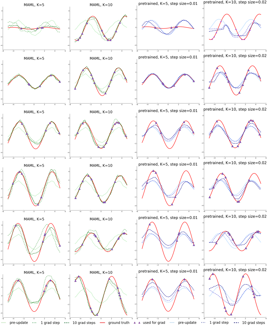
### Visual Description
## Chart Type: Multiple Line Plots
### Overview
The image presents a grid of line plots comparing the performance of MAML (Model-Agnostic Meta-Learning) and a pretrained model under different conditions. The plots show how the model's prediction evolves with gradient steps, compared to the ground truth. The columns represent different configurations of the models (MAML with K=5, MAML with K=10, pretrained with K=5 and step size 0.01, and pretrained with K=10 and step size 0.02). The rows likely represent different tasks or iterations.
### Components/Axes
* **X-axis:** The x-axis is consistent across all plots, ranging from approximately -6 to 6. It is not explicitly labeled, but it likely represents the input to the function being learned.
* **Y-axis:** The y-axis is consistent across all plots, ranging from approximately -4 to 4. It likely represents the output of the function being learned.
* **Plot Titles:** Each plot has a title indicating the model and its configuration:
* "MAML, K=5"
* "MAML, K=10"
* "pretrained, K=5, step size=0.01"
* "pretrained, K=10, step size=0.02"
* **Legend:** Located at the bottom of the image.
* "pre-update": Light green dotted line
* "1 grad step": Black dotted line
* "10 grad steps": Dark blue dotted line
* "ground truth": Red solid line
* "used for grad": Purple triangle markers
### Detailed Analysis
Each plot contains the following data series:
* **Ground Truth (Red solid line):** Represents the target function that the model is trying to learn. It appears to be a sine wave.
* **Pre-update (Light green dotted line):** Represents the model's prediction before any gradient updates.
* **1 grad step (Black dotted line):** Represents the model's prediction after one gradient update.
* **10 grad steps (Dark blue dotted line):** Represents the model's prediction after ten gradient updates.
* **Used for grad (Purple triangle markers):** Indicates the data points used for gradient calculation.
**Observations for each model type:**
* **MAML (K=5 and K=10):**
* The "pre-update" line (light green) is initially far from the "ground truth" (red).
* After 1 gradient step (black), the prediction moves closer to the ground truth.
* After 10 gradient steps (dark blue), the prediction is generally closer to the ground truth than after 1 step, but there are variations across rows.
* The MAML models seem to adapt reasonably well to the target function, with K=10 generally showing a slightly better fit than K=5.
* **Pretrained (K=5, step size=0.01 and K=10, step size=0.02):**
* The "pre-update" line (light green) starts closer to the ground truth (red) compared to MAML.
* After 1 gradient step (black), the prediction moves closer to the ground truth.
* After 10 gradient steps (dark blue), the prediction can overshoot or oscillate around the ground truth, especially with the larger step size (0.02).
* The pretrained models can converge faster initially, but may be more prone to instability or overfitting with more gradient steps.
**Row-wise observations:**
* The rows show different instances or tasks. The performance of each model varies across these tasks, indicating the adaptability of the models to different target functions.
* In some rows, the "10 grad steps" line closely matches the "ground truth," while in others, it deviates significantly, suggesting that the number of steps needed for convergence depends on the specific task.
### Key Observations
* MAML models start with a random initialization and adapt to the target function through gradient updates.
* Pretrained models start with a better initial guess but can be more sensitive to the step size and may overfit or oscillate.
* The number of gradient steps required for convergence varies depending on the task.
* The purple triangles indicate the data points used for gradient calculation, and their placement influences the model's learning.
### Interpretation
The plots demonstrate the trade-offs between MAML and pretrained models. MAML is more flexible and can adapt to a wider range of tasks, but it requires more gradient steps to converge. Pretrained models can converge faster if the initial pretraining is relevant to the task, but they are more sensitive to the step size and may overfit or oscillate. The choice between MAML and a pretrained model depends on the specific application and the availability of pretraining data. The plots also highlight the importance of selecting an appropriate step size and number of gradient steps for optimal performance.
</details>