1706.04599

# On Calibration of Modern Neural Networks **Authors**: Chuan Guo, Geoff Pleiss, Yu Sun, Kilian Q. Weinberger ## On Calibration of Modern Neural Networks Chuan Guo * 1 Geoff Pleiss * 1 Yu Sun * 1 Kilian Q. Weinberger 1 ## Abstract Confidence calibration - the problem of predicting probability estimates representative of the true correctness likelihood -is important for classification models in many applications. We discover that modern neural networks, unlike those from a decade ago, are poorly calibrated. Through extensive experiments, we observe that depth, width, weight decay, and Batch Normalization are important factors influencing calibration. We evaluate the performance of various post-processing calibration methods on state-ofthe-art architectures with image and document classification datasets. Our analysis and experiments not only offer insights into neural network learning, but also provide a simple and straightforward recipe for practical settings: on most datasets, temperature scaling - a singleparameter variant of Platt Scaling - is surprisingly effective at calibrating predictions. ## 1. Introduction Recent advances in deep learning have dramatically improved neural network accuracy (Simonyan & Zisserman, 2015; Srivastava et al., 2015; He et al., 2016; Huang et al., 2016; 2017). As a result, neural networks are now entrusted with making complex decisions in applications, such as object detection (Girshick, 2015), speech recognition (Hannun et al., 2014), and medical diagnosis (Caruana et al., 2015). In these settings, neural networks are an essential component of larger decision making pipelines. In real-world decision making systems, classification networks must not only be accurate, but also should indicate when they are likely to be incorrect. As an example, consider a self-driving car that uses a neural network to detect pedestrians and other obstructions (Bojarski et al., 2016). * Equal contribution, alphabetical order. 1 Cornell University. Correspondence to: Chuan Guo < cg563@cornell.edu > , Geoff Pleiss < geoff@cs.cornell.edu > , Yu Sun < ys646@cornell.edu > . Proceedings of the 34 th International Conference on Machine Learning , Sydney, Australia, PMLR 70, 2017. Copyright 2017 by the author(s). <details> <summary>Image 1 Details</summary>  ### Visual Description ## Bar Chart: Model Performance on CIFAR-100 Dataset ### Overview The image contains two side-by-side bar charts comparing the performance of two neural network architectures (LeNet 1998 and ResNet 2016) on the CIFAR-100 dataset. Each chart has two subplots: (1) Accuracy vs. Confidence distribution, and (2) Output-Gap distribution with error metrics. The charts use stacked bars to show the relationship between model confidence and accuracy, with color-coded legends for "Outputs" (blue) and "Gap" (pink). ### Components/Axes - **X-axis (Confidence)**: Labeled "Confidence" with ticks at 0.0, 0.2, 0.4, 0.6, 0.8, 1.0 - **Y-axis (Left)**: Labeled "% of Samples" for the top subplots, "Accuracy" for the bottom subplots - **Y-axis (Right)**: Implied scale for gap values (not explicitly labeled) - **Legends**: - Blue = "Outputs" - Pink = "Gap" - **Annotations**: - "Avg. confidence" (dashed vertical line) - "Avg. accuracy" (dashed horizontal line) - Error percentages: "Error=44.9" (LeNet), "Error=30.6" (ResNet) ### Detailed Analysis #### LeNet (1998) Chart - **Accuracy vs. Confidence**: - Blue bars (Outputs) show increasing accuracy with confidence, peaking near 1.0 confidence. - Pink bars (Gap) remain minimal across confidence levels. - Average confidence ≈ 0.7 (dashed line), average accuracy ≈ 0.85 (dashed line). - **Output-Gap Distribution**: - Error=44.9% (text annotation at bottom). - Pink bars dominate at lower confidence levels (<0.4), shrinking as confidence increases. #### ResNet (2016) Chart - **Accuracy vs. Confidence**: - Blue bars (Outputs) show near-perfect accuracy (>0.95) at confidence >0.6. - Pink bars (Gap) are negligible across all confidence levels. - Average confidence ≈ 0.85 (dashed line), average accuracy ≈ 0.95 (dashed line). - **Output-Gap Distribution**: - Error=30.6% (text annotation at bottom). - Pink bars are minimal even at low confidence levels (<0.2). ### Key Observations 1. **Model Performance**: - ResNet achieves significantly higher accuracy (≈95%) compared to LeNet (≈85%) at high confidence levels. - ResNet maintains low error (30.6%) vs. LeNet's 44.9%, indicating better calibration. 2. **Confidence-Accuracy Relationship**: - Both models show positive correlation between confidence and accuracy. - ResNet's accuracy plateaus near 1.0 at confidence >0.8, while LeNet plateaus near 0.9. 3. **Output-Gap Behavior**: - LeNet exhibits larger gaps at low confidence levels (<0.4), suggesting poor calibration. - ResNet's gaps remain consistently small across all confidence levels. ### Interpretation The data demonstrates ResNet's superior performance on CIFAR-100 compared to LeNet. ResNet's lower error percentage (30.6% vs. 44.9%) indicates better alignment between model confidence and actual accuracy, particularly at high confidence thresholds. The minimal gap between "Outputs" and "Gap" in ResNet suggests more reliable predictions, while LeNet's larger gaps at low confidence levels highlight potential overconfidence in uncertain regions. These results align with ResNet's architectural advantages (e.g., residual connections) enabling deeper networks to learn more robust features for complex datasets like CIFAR-100. 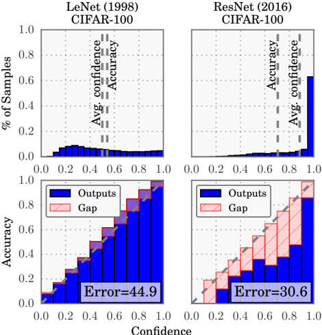</details> Confidence Figure 1. Confidence histograms (top) and reliability diagrams (bottom) for a 5-layer LeNet (left) and a 110-layer ResNet (right) on CIFAR-100. Refer to the text below for detailed illustration. If the detection network is not able to confidently predict the presence or absence of immediate obstructions, the car should rely more on the output of other sensors for braking. Alternatively, in automated health care, control should be passed on to human doctors when the confidence of a disease diagnosis network is low (Jiang et al., 2012). Specifically, a network should provide a calibrated confidence measure in addition to its prediction. In other words, the probability associated with the predicted class label should reflect its ground truth correctness likelihood. Calibrated confidence estimates are also important for model interpretability. Humans have a natural cognitive intuition for probabilities (Cosmides & Tooby, 1996). Good confidence estimates provide a valuable extra bit of information to establish trustworthiness with the user - especially for neural networks, whose classification decisions are often difficult to interpret. Further, good probability estimates can be used to incorporate neural networks into other probabilistic models. For example, one can improve performance by combining network outputs with a lan- guage model in speech recognition (Hannun et al., 2014; Xiong et al., 2016), or with camera information for object detection (Kendall & Cipolla, 2016). In 2005, Niculescu-Mizil & Caruana (2005) showed that neural networks typically produce well-calibrated probabilities on binary classification tasks. While neural networks today are undoubtedly more accurate than they were a decade ago, we discover with great surprise that modern neural networks are no longer well-calibrated . This is visualized in Figure 1, which compares a 5-layer LeNet (left) (LeCun et al., 1998) with a 110-layer ResNet (right) (He et al., 2016) on the CIFAR-100 dataset. The top row shows the distribution of prediction confidence (i.e. probabilities associated with the predicted label) as histograms. The average confidence of LeNet closely matches its accuracy, while the average confidence of the ResNet is substantially higher than its accuracy. This is further illustrated in the bottom row reliability diagrams (DeGroot & Fienberg, 1983; Niculescu-Mizil & Caruana, 2005), which show accuracy as a function of confidence. We see that LeNet is well-calibrated, as confidence closely approximates the expected accuracy (i.e. the bars align roughly along the diagonal). On the other hand, the ResNet's accuracy is better, but does not match its confidence. Our goal is not only to understand why neural networks have become miscalibrated, but also to identify what methods can alleviate this problem. In this paper, we demonstrate on several computer vision and NLP tasks that neural networks produce confidences that do not represent true probabilities. Additionally, we offer insight and intuition into network training and architectural trends that may cause miscalibration. Finally, we compare various postprocessing calibration methods on state-of-the-art neural networks, and introduce several extensions of our own. Surprisingly, we find that a single-parameter variant of Platt scaling (Platt et al., 1999) - which we refer to as temperature scaling - is often the most effective method at obtaining calibrated probabilities. Because this method is straightforward to implement with existing deep learning frameworks, it can be easily adopted in practical settings. ## 2. Definitions The problem we address in this paper is supervised multiclass classification with neural networks. The input X ∈ X and label Y ∈ Y = { 1 , . . . , K } are random variables that follow a ground truth joint distribution π ( X,Y ) = π ( Y | X ) π ( X ) . Let h be a neural network with h ( X ) = ( ˆ Y , ˆ P ) , where ˆ Y is a class prediction and ˆ P is its associated confidence, i.e. probability of correctness. We would like the confidence estimate ˆ P to be calibrated, which intuitively means that ˆ P represents a true probability. For example, given 100 predictions, each with confidence of 0 . 8 , we expect that 80 should be correctly classified. More formally, we define perfect calibration as $$( \hat { Y } = Y | P = p ) =$$ where the probability is over the joint distribution. In all practical settings, achieving perfect calibration is impossible. Additionally, the probability in (1) cannot be computed using finitely many samples since ˆ P is a continuous random variable. This motivates the need for empirical approximations that capture the essence of (1). Reliability Diagrams (e.g. Figure 1 bottom) are a visual representation of model calibration (DeGroot & Fienberg, 1983; Niculescu-Mizil & Caruana, 2005). These diagrams plot expected sample accuracy as a function of confidence. If the model is perfectly calibrated - i.e. if (1) holds - then the diagram should plot the identity function. Any deviation from a perfect diagonal represents miscalibration. To estimate the expected accuracy from finite samples, we group predictions into M interval bins (each of size 1 /M ) and calculate the accuracy of each bin. Let B m be the set of indices of samples whose prediction confidence falls into the interval I m = ( m -1 M , m M ] . The accuracy of B m is $$\frac { 1 } { \vert B _ { m } \vert } = \sum _ { i \in B _ { m } } ^ { 1 } I ( b _ { i } - a _ { i } ) ,$$ where ˆ y i and y i are the predicted and true class labels for sample i . Basic probability tells us that acc( B m ) is an unbiased and consistent estimator of P ( ˆ Y = Y | ˆ P ∈ I m ) . We define the average confidence within bin B m as $$\cos ( B _ { m } ) = \frac { 1 } { \vert B _ { m } \vert } \sum _ { i \in B _ { m } } ^ { 1 } p _ { i }$$ where ˆ p i is the confidence for sample i . acc( B m ) and conf( B m ) approximate the left-hand and right-hand sides of (1) respectively for bin B m . Therefore, a perfectly calibrated model will have acc( B m ) = conf( B m ) for all m ∈ { 1 , . . . , M } . Note that reliability diagrams do not display the proportion of samples in a given bin, and thus cannot be used to estimate how many samples are calibrated. Expected Calibration Error (ECE). While reliability diagrams are useful visual tools, it is more convenient to have a scalar summary statistic of calibration. Since statistics comparing two distributions cannot be comprehensive, previous works have proposed variants, each with a unique emphasis. One notion of miscalibration is the difference in expectation between confidence and accuracy, i.e. 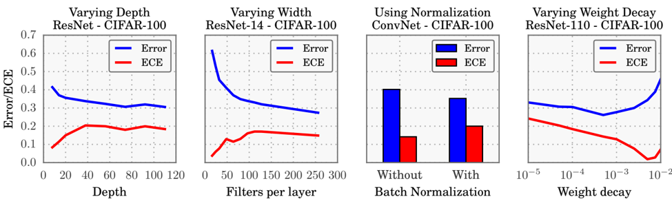$$\frac { \int | p ( y = y | P = } _ { p } } { | p | } - | p | } ( 2 )$$ Expected Calibration Error (Naeini et al., 2015) - or ECE -approximates (2) by partitioning predictions into M equally-spaced bins (similar to the reliability diagrams) and Figure 2. The effect of network depth (far left), width (middle left), Batch Normalization (middle right), and weight decay (far right) on miscalibration, as measured by ECE (lower is better). <details> <summary>Image 2 Details</summary>  ### Visual Description ## Line Graphs and Bar Chart: Model Performance on CIFAR-100 ### Overview The image contains four visualizations comparing model performance metrics (Error and Expected Calibration Error, ECE) on the CIFAR-100 dataset. Each graph explores the impact of architectural or training parameter variations: depth, width, batch normalization, and weight decay. Data is presented as line graphs (for continuous parameters) and a bar chart (for binary comparison). --- ### Components/Axes 1. **Graph 1: Varying Depth (ResNet-CIFAR-100)** - **X-axis**: Depth (0–120 layers) - **Y-axis**: Error/ECE (0.0–0.7) - **Legend**: Blue = Error, Red = ECE - **Legend Position**: Top-right corner 2. **Graph 2: Varying Width (ResNet-14-CIFAR-100)** - **X-axis**: Filters per layer (0–300) - **Y-axis**: Error/ECE (0.0–0.7) - **Legend**: Blue = Error, Red = ECE - **Legend Position**: Top-right corner 3. **Graph 3: Batch Normalization (ConvNet-CIFAR-100)** - **X-axis**: Binary categories ("Without", "With") - **Y-axis**: Error/ECE (0.0–0.7) - **Legend**: Blue = Error, Red = ECE - **Legend Position**: Top-right corner 4. **Graph 4: Varying Weight Decay (ResNet-110-CIFAR-100)** - **X-axis**: Weight decay (10⁻⁵ to 10⁻²) - **Y-axis**: Error/ECE (0.0–0.7) - **Legend**: Blue = Error, Red = ECE - **Legend Position**: Top-right corner --- ### Detailed Analysis #### Graph 1: Varying Depth - **Error (Blue Line)**: Starts at ~0.4, decreases to ~0.3 by depth 60, then stabilizes. - **ECE (Red Line)**: Peaks at ~0.2 at depth 40, then declines to ~0.1 by depth 120. - **Key Data Points**: - Depth 0: Error = 0.4, ECE = 0.1 - Depth 60: Error = 0.3, ECE = 0.15 - Depth 120: Error = 0.3, ECE = 0.1 #### Graph 2: Varying Width - **Error (Blue Line)**: Starts at ~0.6, drops sharply to ~0.3 by 150 filters, then plateaus. - **ECE (Red Line)**: Peaks at ~0.2 at 50 filters, then declines to ~0.1 by 300 filters. - **Key Data Points**: - 0 filters: Error = 0.6, ECE = 0.1 - 150 filters: Error = 0.3, ECE = 0.15 - 300 filters: Error = 0.3, ECE = 0.1 #### Graph 3: Batch Normalization - **Without BN**: - Error = 0.4 - ECE = 0.2 - **With BN**: - Error = 0.3 - ECE = 0.1 - **Observation**: Batch normalization reduces both error and ECE by ~25%. #### Graph 4: Varying Weight Decay - **Error (Blue Line)**: U-shaped curve. Starts at ~0.3 (10⁻⁵), dips to ~0.2 (10⁻³), then rises to ~0.4 (10⁻²). - **ECE (Red Line)**: V-shaped curve. Starts at ~0.2 (10⁻⁵), drops to ~0.1 (10⁻³), then rises to ~0.2 (10⁻²). - **Key Data Points**: - 10⁻⁵: Error = 0.3, ECE = 0.2 - 10⁻³: Error = 0.2, ECE = 0.1 - 10⁻²: Error = 0.4, ECE = 0.2 --- ### Key Observations 1. **Depth vs. Width**: Increasing depth (Graph 1) and width (Graph 2) both reduce error, but ECE initially increases before stabilizing. 2. **Batch Normalization**: Significantly improves calibration (ECE drops from 0.2 to 0.1) and reduces error. 3. **Weight Decay**: Optimal performance occurs at moderate decay (10⁻³), with both error and ECE minimized. --- ### Interpretation - **Depth/Width Trade-offs**: Deeper/wider networks improve accuracy but may overfit (higher ECE initially). However, ECE stabilizes as models become sufficiently complex. - **Batch Normalization**: Critical for reducing both error and calibration error, suggesting it mitigates overconfidence in predictions. - **Weight Decay**: Moderate regularization (10⁻³) balances model complexity and generalization. Extreme values (10⁻⁵ or 10⁻²) degrade performance, likely due to underfitting or overfitting. - **Model Architecture**: ResNet variants (14, 110 layers) and ConvNet show similar trends, but ResNets handle deeper architectures better (Graph 1 vs. Graph 4). This analysis highlights the interplay between architectural choices and training hyperparameters in achieving robust performance on CIFAR-100. </details> taking a weighted average of the bins' accuracy/confidence difference. More precisely, $$\sum _ { m = 1 } ^ { M } \frac { | B _ { m } | } { n } | a c c ( B _ { m } ) |$$ where n is the number of samples. The difference between acc and conf for a given bin represents the calibration gap (red bars in reliability diagrams - e.g. Figure 1). We use ECE as the primary empirical metric to measure calibration. See Section S1 for more analysis of this metric. Maximum Calibration Error (MCE). In high-risk applications where reliable confidence measures are absolutely necessary, we may wish to minimize the worst-case deviation between confidence and accuracy: $$\max _ { p \in [0 , 1 ] } | p ( Y = Y | P ) - p | .$$ The Maximum Calibration Error (Naeini et al., 2015) - or MCE - estimates this deviation. Similarly to ECE, this approximation involves binning: $$\frac { M C E } { B _ { m } } = \max _ { M \in \{ 1 , \ldots , M \} } | a c c ( M ) |$$ We can visualize MCE and ECE on reliability diagrams. MCEis the largest calibration gap (red bars) across all bins, whereas ECE is a weighted average of all gaps. For perfectly calibrated classifiers, MCE and ECE both equal 0. Negative log likelihood is a standard measure of a probabilistic model's quality (Friedman et al., 2001). It is also referred to as the cross entropy loss in the context of deep learning (Bengio et al., 2015). Given a probabilistic model ˆ π ( Y | X ) and n samples, NLL is defined as: $$C = - \sum _ { i = 1 } ^ { n } \log ( x _ { i } | y _ { i } | x _ { j } )$$ It is a standard result (Friedman et al., 2001) that, in expectation, NLL is minimized if and only if ˆ π ( Y | X ) recovers the ground truth conditional distribution π ( Y | X ) . ## 3. Observing Miscalibration The architecture and training procedures of neural networks have rapidly evolved in recent years. In this section we identify some recent changes that are responsible for the miscalibration phenomenon observed in Figure 1. Though we cannot claim causality, we find that increased model capacity and lack of regularization are closely related to model miscalibration. Model capacity. The model capacity of neural networks has increased at a dramatic pace over the past few years. It is now common to see networks with hundreds, if not thousands of layers (He et al., 2016; Huang et al., 2016) and hundreds of convolutional filters per layer (Zagoruyko & Komodakis, 2016). Recent work shows that very deep or wide models are able to generalize better than smaller ones, while exhibiting the capacity to easily fit the training set (Zhang et al., 2017). Although increasing depth and width may reduce classification error, we observe that these increases negatively affect model calibration. Figure 2 displays error and ECE as a function of depth and width on a ResNet trained on CIFAR-100. The far left figure varies depth for a network with 64 convolutional filters per layer, while the middle left figure fixes the depth at 14 layers and varies the number of convolutional filters per layer. Though even the smallest models in the graph exhibit some degree of miscalibration, the ECE metric grows substantially with model capacity. During training, after the model is able to correctly classify (almost) all training samples, NLL can be further minimized by increasing the confidence of predictions. Increased model capacity will lower training NLL, and thus the model will be more (over)confident on average. 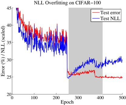Batch Normalization (Ioffe & Szegedy, 2015) improves the optimization of neural networks by minimizing distribution shifts in activations within the neural network's hid- Figure 3. Test error and NLL of a 110-layer ResNet with stochastic depth on CIFAR-100 during training. NLL is scaled by a constant to fit in the figure. Learning rate drops by 10x at epochs 250 and 375. The shaded area marks between epochs at which the best validation loss and best validation error are produced. <details> <summary>Image 3 Details</summary>  ### Visual Description ## Line Graph: NLL Overfitting on CIFAR-100 ### Overview The image is a line graph comparing two metrics—Test Error and Test NLL—over 500 training epochs during a neural network's training on the CIFAR-100 dataset. The graph highlights overfitting behavior, with a shaded region marking a critical phase in training dynamics. ### Components/Axes - **X-axis (Epoch)**: Labeled "Epoch," ranging from 0 to 500 in increments of 100. - **Y-axis (Error %)**: Labeled "Error (%) / NLL (scaled)," ranging from 20% to 45% in increments of 5%. - **Legend**: Located in the top-right corner, with: - **Red line**: "Test error" - **Blue line**: "Test NLL" - **Shaded Region**: A gray vertical band spans epochs 250 to 400, likely indicating a phase transition (e.g., overfitting onset). ### Detailed Analysis 1. **Test Error (Red Line)**: - Starts at ~45% at epoch 0. - Decreases sharply to ~35% by epoch 100. - Fluctuates between ~25% and ~35% until epoch 250. - Stabilizes near ~25% from epoch 250 onward, with minor oscillations. - **Key Trend**: Gradual improvement followed by stabilization. 2. **Test NLL (Blue Line)**: - Begins at ~35% at epoch 0. - Drops to ~25% by epoch 250, mirroring the Test Error trend. - Rises sharply to ~30% by epoch 500, with increasing volatility. - **Key Trend**: Initial improvement, followed by divergence and deterioration. 3. **Shaded Region (Epochs 250–400)**: - Coincides with the divergence of the two lines. - Test NLL begins its upward trend here, while Test Error plateaus. ### Key Observations - **Divergence at Epoch 250**: The Test NLL (blue) begins to rise while Test Error (red) stabilizes, suggesting overfitting. - **Test Error Stability**: The red line’s plateau indicates the model’s performance on test data no longer improves significantly after epoch 250. - **Test NLL Volatility**: The blue line’s increasing oscillations after epoch 250 imply growing sensitivity to training data noise. ### Interpretation The graph demonstrates classic overfitting behavior: - **Initial Improvement**: Both metrics improve as the model learns meaningful patterns (epochs 0–250). - **Overfitting Onset**: After epoch 250, the model memorizes training data, causing Test NLL to rise (blue line) while Test Error remains stable (red line). This divergence indicates the model’s loss function (NLL) becomes misaligned with generalization performance. - **Shaded Region Significance**: The gray area marks the critical epoch range where overfitting becomes evident. The Test NLL’s rise suggests the model’s confidence in training data exceeds its ability to generalize, a hallmark of overfitting. **Notable Anomalies**: - Test Error’s minor fluctuations post-epoch 250 may reflect dataset noise or batch-specific variations. - Test NLL’s sharp rise after epoch 400 could indicate further overfitting or dataset-specific challenges (e.g., class imbalance). **Technical Implications**: - The graph underscores the importance of monitoring both loss functions and test error during training. - The divergence between Test Error and Test NLL highlights the need for regularization (e.g., dropout, weight decay) to mitigate overfitting in deep learning pipelines. </details> den layers. Recent research suggests that these normalization techniques have enabled the development of very deep architectures, such as ResNets (He et al., 2016) and DenseNets (Huang et al., 2017). It has been shown that Batch Normalization improves training time, reduces the need for additional regularization, and can in some cases improve the accuracy of networks. While it is difficult to pinpoint exactly how Batch Normalization affects the final predictions of a model, we do observe that models trained with Batch Normalization tend to be more miscalibrated. In the middle right plot of Figure 2, we see that a 6-layer ConvNet obtains worse calibration when Batch Normalization is applied, even though classification accuracy improves slightly. We find that this result holds regardless of the hyperparameters used on the Batch Normalization model (i.e. low or high learning rate, etc.). Weight decay, which used to be the predominant regularization mechanism for neural networks, is decreasingly utilized when training modern neural networks. Learning theory suggests that regularization is necessary to prevent overfitting, especially as model capacity increases (Vapnik, 1998). However, due to the apparent regularization effects of Batch Normalization, recent research seems to suggest that models with less L2 regularization tend to generalize better (Ioffe & Szegedy, 2015). As a result, it is now common to train models with little weight decay, if any at all. The top performing ImageNet models of 2015 all use an order of magnitude less weight decay than models of previous years (He et al., 2016; Simonyan & Zisserman, 2015). We find that training with less weight decay has a negative impact on calibration. The far right plot in Figure 2 dis- plays training error and ECE for a 110-layer ResNet with varying amounts of weight decay. The only other forms of regularization are data augmentation and Batch Normalization. We observe that calibration and accuracy are not optimized by the same parameter setting. While the model exhibits both over-regularization and under-regularization with respect to classification error, it does not appear that calibration is negatively impacted by having too much weight decay. Model calibration continues to improve when more regularization is added, well after the point of achieving optimal accuracy. The slight uptick at the end of the graph may be an artifact of using a weight decay factor that impedes optimization. NLL can be used to indirectly measure model calibration. In practice, we observe a disconnect between NLL and accuracy , which may explain the miscalibration in Figure 2. This disconnect occurs because neural networks can overfit to NLL without overfitting to the 0/1 loss . We observe this trend in the training curves of some miscalibrated models. Figure 3 shows test error and NLL (rescaled to match error) on CIFAR-100 as training progresses. Both error and NLL immediately drop at epoch 250, when the learning rate is dropped; however, NLL overfits during the remainder of training. Surprisingly, overfitting to NLL is beneficial to classification accuracy. On CIFAR-100, test error drops from 29% to 27% in the region where NLL overfits. This phenomenon renders a concrete explanation of miscalibration: the network learns better classification accuracy at the expense of well-modeled probabilities. We can connect this finding to recent work examining the generalization of large neural networks. Zhang et al. (2017) observe that deep neural networks seemingly violate the common understanding of learning theory that large models with little regularization will not generalize well. The observed disconnect between NLL and 0/1 loss suggests that these high capacity models are not necessarily immune from overfitting, but rather, overfitting manifests in probabilistic error rather than classification error. ## 4. Calibration Methods In this section, we first review existing calibration methods, and introduce new variants of our own. All methods are post-processing steps that produce (calibrated) probabilities. Each method requires a hold-out validation set, which in practice can be the same set used for hyperparameter tuning. We assume that the training, validation, and test sets are drawn from the same distribution. ## 4.1. Calibrating Binary Models We first introduce calibration in the binary setting, i.e. Y = { 0 , 1 } . For simplicity, throughout this subsection, we assume the model outputs only the confidence for the positive class. 1 Given a sample x i , we have access to ˆ p i -the network's predicted probability of y i = 1 , as well as z i ∈ R - which is the network's non-probabilistic output, or logit . The predicted probability ˆ p i is derived from z i using a sigmoid function σ ; i.e. ˆ p i = σ ( z i ) . Our goal is to produce a calibrated probability ˆ q i based on y i , ˆ p i , and z i . Histogram binning (Zadrozny & Elkan, 2001) is a simple non-parametric calibration method. In a nutshell, all uncalibrated predictions ˆ p i are divided into mutually exclusive bins B 1 , . . . , B M . Each bin is assigned a calibrated score θ m ; i.e. if ˆ p i is assigned to bin B m , then ˆ q i = θ m . At test time, if prediction ˆ p te falls into bin B m , then the calibrated prediction ˆ q te is θ m . More precisely, for a suitably chosen M (usually small), we first define bin boundaries 0 = a 1 ≤ a 2 ≤ . . . ≤ a M +1 = 1 , where the bin B m is defined by the interval ( a m , a m +1 ] . Typically the bin boundaries are either chosen to be equal length intervals or to equalize the number of samples in each bin. The predictions θ i are chosen to minimize the bin-wise squared loss: $$\sum _ { m = 1 } ^ { \infty } \sum _ { n = 1 } ^ { M } 1 ( a _ { m } - \hat { p } _ { n } ) ^ { 2 } , ( T )$$ where 1 is the indicator function. Given fixed bins boundaries, the solution to (7) results in θ m that correspond to the average number of positive-class samples in bin B m . Isotonic regression (Zadrozny & Elkan, 2002), arguably the most common non-parametric calibration method, learns a piecewise constant function f to transform uncalibrated outputs; i.e. ˆ q i = f (ˆ p i ) . Specifically, isotonic regression produces f to minimize the square loss ∑ n i =1 ( f (ˆ p i ) -y i ) 2 . Because f is constrained to be piecewise constant, we can write the optimization problem as: $$\min _ { \theta _ { 1 } , \ldots , \theta _ { M } , a _ { 1 } , \ldots , a _ { M + 1 } } \sum _ { m = 1 } ^ { n } \sum _ { i = 1 } ^ { n } 1 ( a _ { m } - \theta _ { m } ) ( \theta _ { m } - y _ { i } ) ^ { 2 }$$ where M is the number of intervals; a 1 , . . . , a M +1 are the interval boundaries; and θ 1 , . . . , θ M are the function values. Under this parameterization, isotonic regression is a strict generalization of histogram binning in which the bin boundaries and bin predictions are jointly optimized. Bayesian Binning into Quantiles (BBQ) (Naeini et al., 2015) is a extension of histogram binning using Bayesian 1 This is in contrast with the setting in Section 2, in which the model produces both a class prediction and confidence. model averaging. Essentially, BBQ marginalizes out all possible binning schemes to produce ˆ q i . More formally, a binning scheme s is a pair ( M, I ) where M is the number of bins, and I is a corresponding partitioning of [0 , 1] into disjoint intervals ( 0 = a 1 ≤ a 2 ≤ . . . ≤ a M +1 = 1 ). The parameters of a binning scheme are θ 1 , . . . , θ M . Under this framework, histogram binning and isotonic regression both produce a single binning scheme, whereas BBQ considers a space S of all possible binning schemes for the validation dataset D . BBQ performs Bayesian averaging of the probabilities produced by each scheme: 2 $$\begin{aligned} P ( q _ { te } | p _ { te } , D ) & = \sum _ { s \in S } P ( q _ { te } , s = s, D ) \\ & = \sum _ { s \in S } P ( q _ { te } , s = s, D ) . \end{aligned}$$ where P (ˆ q te | ˆ p te , S = s, D ) is the calibrated probability using binning scheme s . Using a uniform prior, the weight P ( S = s | D ) can be derived using Bayes' rule: $$P ( S = s | D ) = \frac { P ( D | S = s ) } { \sum _ { s \in S } P ( D | S = s ) }$$ The parameters θ 1 , . . . , θ M can be viewed as parameters of M independent binomial distributions. Hence, by placing a Beta prior on θ 1 , . . . , θ M , we can obtain a closed form expression for the marginal likelihood P ( D | S = s ) . This allows us to compute P (ˆ q te | ˆ p te , D ) for any test input. Platt scaling (Platt et al., 1999) is a parametric approach to calibration, unlike the other approaches. The nonprobabilistic predictions of a classifier are used as features for a logistic regression model, which is trained on the validation set to return probabilities. More specifically, in the context of neural networks (Niculescu-Mizil & Caruana, 2005), Platt scaling learns scalar parameters a, b ∈ R and outputs ˆ q i = σ ( az i + b ) as the calibrated probability. Parameters a and b can be optimized using the NLL loss over the validation set. It is important to note that the neural network's parameters are fixed during this stage. ## 4.2. Extension to Multiclass Models For classification problems involving K > 2 classes, we return to the original problem formulation. The network outputs a class prediction ˆ y i and confidence score ˆ p i for each input x i . In this case, the network logits z i are vectors, where ˆ y i = argmax k z ( k ) i , and ˆ p i is typically derived using the softmax function σ SM: $$\sigma _ { SM } ( z _ { i } ) ^ { k } = \frac { e x p ( z _ { i } ) } { \sum _ { j = 1 } ^ { k } e x p ( z _ { i } , t ) } .$$ The goal is to produce a calibrated confidence ˆ q i and (possibly new) class prediction ˆ y ′ i based on y i , ˆ y i , ˆ p i , and z i . 2 Because the validation dataset is finite, S is as well. Table 1. ECE (%) (with M = 15 bins) on standard vision and NLP datasets before calibration and with various calibration methods. The number following a model's name denotes the network depth. | Dataset | Model | Uncalibrated | Hist. Binning | Isotonic | BBQ | Temp. Scaling | Vector Scaling | Matrix Scaling | |------------------|-----------------|----------------|-----------------|------------|-------|-----------------|------------------|------------------| | Birds | ResNet 50 | 9.19% | 4.34% | 5.22% | 4.12% | 1.85% | 3.0% | 21.13% | | Cars | ResNet 50 | 4.3% | 1.74% | 4.29% | 1.84% | 2.35% | 2.37% | 10.5% | | CIFAR-10 | ResNet 110 | 4.6% | 0.58% | 0.81% | 0.54% | 0.83% | 0.88% | 1.0% | | CIFAR-10 | ResNet 110 (SD) | 4.12% | 0.67% | 1.11% | 0.9% | 0.6% | 0.64% | 0.72% | | CIFAR-10 | Wide ResNet 32 | 4.52% | 0.72% | 1.08% | 0.74% | 0.54% | 0.6% | 0.72% | | CIFAR-10 | DenseNet 40 | 3.28% | 0.44% | 0.61% | 0.81% | 0.33% | 0.41% | 0.41% | | CIFAR-10 | LeNet 5 | 3.02% | 1.56% | 1.85% | 1.59% | 0.93% | 1.15% | 1.16% | | CIFAR-100 | ResNet 110 | 16.53% | 2.66% | 4.99% | 5.46% | 1.26% | 1.32% | 25.49% | | CIFAR-100 | ResNet 110 (SD) | 12.67% | 2.46% | 4.16% | 3.58% | 0.96% | 0.9% | 20.09% | | CIFAR-100 | Wide ResNet 32 | 15.0% | 3.01% | 5.85% | 5.77% | 2.32% | 2.57% | 24.44% | | CIFAR-100 | DenseNet 40 | 10.37% | 2.68% | 4.51% | 3.59% | 1.18% | 1.09% | 21.87% | | CIFAR-100 | LeNet 5 | 4.85% | 6.48% | 2.35% | 3.77% | 2.02% | 2.09% | 13.24% | | ImageNet | DenseNet 161 | 6.28% | 4.52% | 5.18% | 3.51% | 1.99% | 2.24% | - | | ImageNet | ResNet 152 | 5.48% | 4.36% | 4.77% | 3.56% | 1.86% | 2.23% | - | | SVHN | ResNet 152 (SD) | 0.44% | 0.14% | 0.28% | 0.22% | 0.17% | 0.27% | 0.17% | | 20 News | DAN 3 | 8.02% | 3.6% | 5.52% | 4.98% | 4.11% | 4.61% | 9.1% | | Reuters | DAN 3 | 0.85% | 1.75% | 1.15% | 0.97% | 0.91% | 0.66% | 1.58% | | SST Binary | TreeLSTM | 6.63% | 1.93% | 1.65% | 2.27% | 1.84% | 1.84% | 1.84% | | SST Fine Grained | TreeLSTM | 6.71% | 2.09% | 1.65% | 2.61% | 2.56% | 2.98% | 2.39% | Extension of binning methods. One common way of extending binary calibration methods to the multiclass setting is by treating the problem as K one-versus-all problems (Zadrozny & Elkan, 2002). For k = 1 , . . . , K , we form a binary calibration problem where the label is 1 ( y i = k ) and the predicted probability is σ SM ( z i ) ( k ) . This gives us K calibration models, each for a particular class. At test time, we obtain an unnormalized probability vector [ˆ q (1) i , . . . , ˆ q ( K ) i ] , where ˆ q ( k ) i is the calibrated probability for class k . The new class prediction ˆ y ′ i is the argmax of the vector, and the new confidence ˆ q ′ i is the max of the vector normalized by ∑ K k =1 ˆ q ( k ) i . This extension can be applied to histogram binning, isotonic regression, and BBQ. Matrix and vector scaling are two multi-class extensions of Platt scaling. Let z i be the logits vector produced before the softmax layer for input x i . Matrix scaling applies a linear transformation Wz i + b to the logits: $$q _ { i } = \max _ { k } o s M ( W z _ { i } + b ) ^ { k } , q _ { i } = \arg m a x ( W z _ { i } + b ) ^ { k }$$ The parameters W and b are optimized with respect to NLL on the validation set. As the number of parameters for matrix scaling grows quadratically with the number of classes K , we define vector scaling as a variant where W is restricted to be a diagonal matrix. Temperature scaling, the simplest extension of Platt scaling, uses a single scalar parameter T > 0 for all classes. Given the logit vector z i , the new confidence prediction is $$i = m _ { 1 } \times m _ { 2 } ( 7 ^ { n - 1 } ) ^ { 1 } , \ldots$$ T is called the temperature, and it 'softens' the softmax (i.e. raises the output entropy) with T > 1 . As T → ∞ , the probability ˆ q i approaches 1 /K , which represents maximum uncertainty. With T = 1 , we recover the original probability ˆ p i . As T → 0 , the probability collapses to a point mass (i.e. ˆ q i = 1 ). T is optimized with respect to NLL on the validation set. Because the parameter T does not change the maximum of the softmax function, the class prediction ˆ y ′ i remains unchanged. In other words, temperature scaling does not affect the model's accuracy. Temperature scaling is commonly used in settings such as knowledge distillation (Hinton et al., 2015) and statistical mechanics (Jaynes, 1957). To the best of our knowledge, we are not aware of any prior use in the context of calibrating probabilistic models. 3 The model is equivalent to maximizing the entropy of the output probability distribution subject to certain constraints on the logits (see Section S2). ## 4.3. Other Related Works Calibration and confidence scores have been studied in various contexts in recent years. Kuleshov & Ermon (2016) study the problem of calibration in the online setting, where the inputs can come from a potentially adversarial source. Kuleshov & Liang (2015) investigate how to produce calibrated probabilities when the output space is a structured object. Lakshminarayanan et al. (2016) use ensembles of networks to obtain uncertainty estimates. Pereyra et al. (2017) penalize overconfident predictions as a form of regularization. Hendrycks & Gimpel (2017) use confidence 3 To highlight the connection with prior works we define temperature scaling in terms of 1 T instead of a multiplicative scalar. scores to determine if samples are out-of-distribution. Bayesian neural networks (Denker & Lecun, 1990; MacKay, 1992) return a probability distribution over outputs as an alternative way to represent model uncertainty. Gal & Ghahramani (2016) draw a connection between Dropout (Srivastava et al., 2014) and model uncertainty, claiming that sampling models with dropped nodes is a way to estimate the probability distribution over all possible models for a given sample. Kendall & Gal (2017) combine this approach with a model that outputs a predictive mean and variance for each data point. This notion of uncertainty is not restricted to classification problems. Additionally, neural networks can be used in conjunction with Bayesian models that output complete distributions. For example, deep kernel learning (Wilson et al., 2016a;b; AlShedivat et al., 2016) combines deep neural networks with Gaussian processes on classification and regression problems. In contrast, our framework, which does not augment the neural network model, returns a confidence score rather than returning a distribution of possible outputs. ## 5. Results We apply the calibration methods in Section 4 to image classification and document classification neural networks. For image classification we use 6 datasets: 1. Caltech-UCSD Birds (Welinder et al., 2010): 200 bird species. 5994/2897/2897 images for train/validation/test sets. 2. Stanford Cars (Krause et al., 2013): 196 classes of cars by make, model, and year. 8041/4020/4020 images for train/validation/test. 3. ImageNet 2012 (Deng et al., 2009): Natural scene images from 1000 classes. 1.3 million/25,000/25,000 images for train/validation/test. 4. CIFAR-10/CIFAR-100 (Krizhevsky & Hinton, 2009): Color images ( 32 × 32 ) from 10/100 classes. 45,000/5,000/10,000 images for train/validation/test. 5. Street View House Numbers (SVHN) (Netzer et al., 2011): 32 × 32 colored images of cropped out house numbers from Google Street View. 598,388/6,000/26,032 images for train/validation/test. We train state-of-the-art convolutional networks: ResNets (He et al., 2016), ResNets with stochastic depth (SD) (Huang et al., 2016), Wide ResNets (Zagoruyko & Komodakis, 2016), and DenseNets (Huang et al., 2017). We use the data preprocessing, training procedures, and hyperparameters as described in each paper. For Birds and Cars, we fine-tune networks pretrained on ImageNet. For document classification we experiment with 4 datasets: 1. 20 News: News articles, partitioned into 20 cate- 2. gories by content. 9034/2259/7528 documents for train/validation/test. 2. Reuters: News articles, partitioned into 8 categories by topic. 4388/1097/2189 documents for train/validation/test. 3. Stanford Sentiment Treebank (SST) (Socher et al., 2013): Movie reviews, represented as sentence parse trees that are annotated by sentiment. Each sample includes a coarse binary label and a fine grained 5-class label. As described in (Tai et al., 2015), the training/validation/test sets contain 6920/872/1821 documents for binary, and 544/1101/2210 for fine-grained. On 20 News and Reuters, we train Deep Averaging Networks (DANs) (Iyyer et al., 2015) with 3 feed-forward layers and Batch Normalization. On SST, we train TreeLSTMs (Long Short Term Memory) (Tai et al., 2015). For both models we use the default hyperparmaeters suggested by the authors. Calibration Results. Table 1 displays model calibration, as measured by ECE (with M = 15 bins), before and after applying the various methods (see Section S3 for MCE, NLL, and error tables). It is worth noting that most datasets and models experience some degree of miscalibration, with ECE typically between 4 to 10% . This is not architecture specific: we observe miscalibration on convolutional networks (with and without skip connections), recurrent networks, and deep averaging networks. The two notable exceptions are SVHN and Reuters, both of which experience ECE values below 1% . Both of these datasets have very low error ( 1 . 98% and 2 . 97% , respectively); and therefore the ratio of ECE to error is comparable to other datasets. Our most important discovery is the surprising effectiveness of temperature scaling despite its remarkable simplicity. Temperature scaling outperforms all other methods on the vision tasks, and performs comparably to other methods on the NLP datasets. What is perhaps even more surprising is that temperature scaling outperforms the vector and matrix Platt scaling variants, which are strictly more general methods. In fact, vector scaling recovers essentially the same solution as temperature scaling - the learned vector has nearly constant entries, and therefore is no different than a scalar transformation. In other words, network miscalibration is intrinsically low dimensional. The only dataset that temperature scaling does not calibrate is the Reuters dataset. In this instance, only one of the above methods is able to improve calibration. Because this dataset is well-calibrated to begin with (ECE ≤ 1% ), there is not much room for improvement with any method, and post-processing may not even be necessary to begin with. It is also possible that our measurements are affected by dataset split or by the particular binning scheme. 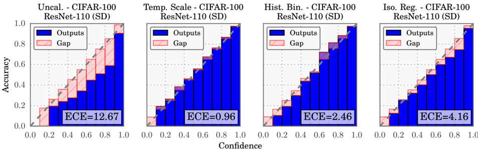Figure 4. Reliability diagrams for CIFAR-100 before (far left) and after calibration (middle left, middle right, far right). <details> <summary>Image 4 Details</summary>  ### Visual Description ## Bar Charts: Calibration Performance of ResNet-110 (SD) on CIFAR-100 ### Overview The image contains four side-by-side bar charts comparing calibration methods for a ResNet-110 (SD) model trained on the CIFAR-100 dataset. Each chart evaluates a different calibration technique: **Uncal.** (uncalibrated), **Temp. Scale** (temperature scaling), **Hist. Bin.** (histogram binning), and **Iso. Reg.** (isotonic regression). The charts visualize the relationship between model confidence and accuracy, with error bars representing uncertainty. --- ### Components/Axes - **X-axis (Confidence)**: Ranges from 0.0 to 1.0 in increments of 0.2. Labeled "Confidence." - **Y-axis (Accuracy)**: Ranges from 0.0 to 1.0 in increments of 0.2. Labeled "Accuracy." - **Legend**: - **Blue bars**: "Outputs" (model accuracy at given confidence levels). - **Pink bars**: "Gap" (difference between confidence and accuracy). - **Chart Titles**: - Top-left: "Uncal. - CIFAR-100 ResNet-110 (SD)" - Top-center-left: "Temp. Scale - CIFAR-100 ResNet-110 (SD)" - Top-center-right: "Hist. Bin. - CIFAR-100 ResNet-110 (SD)" - Top-right: "Iso. Reg. - CIFAR-100 ResNet-110 (SD)" - **ECE Values**: Embedded in the bottom-left corner of each chart: - Uncal.: ECE = 12.67 - Temp. Scale: ECE = 0.96 - Hist. Bin.: ECE = 2.46 - Iso. Reg.: ECE = 4.16 --- ### Detailed Analysis 1. **Uncal. (Uncalibrated)**: - Highest ECE (12.67), indicating severe miscalibration. - Blue bars (Outputs) show accuracy increasing with confidence but lagging behind confidence values. - Pink "Gap" bars are consistently large, especially at higher confidence levels (e.g., 0.8–1.0). 2. **Temp. Scale (Temperature Scaling)**: - Lowest ECE (0.96), suggesting optimal calibration. - Blue bars closely align with confidence values across all levels. - Pink "Gap" bars are minimal, indicating near-perfect alignment between confidence and accuracy. 3. **Hist. Bin. (Histogram Binning)**: - Moderate ECE (2.46). - Blue bars show gradual improvement in accuracy with confidence but with noticeable gaps at mid-to-high confidence levels (e.g., 0.6–0.8). - Pink "Gap" bars are smaller than Uncal. but larger than Temp. Scale. 4. **Iso. Reg. (Isotonic Regression)**: - ECE = 4.16, worse than Hist. Bin. but better than Uncal. - Blue bars exhibit a steeper increase in accuracy at higher confidence levels (e.g., 0.6–1.0). - Pink "Gap" bars are moderate, with larger discrepancies at lower confidence levels (e.g., 0.0–0.4). --- ### Key Observations - **Calibration Trends**: - Uncal. exhibits the largest calibration error (ECE = 12.67), with accuracy consistently below confidence. - Temp. Scale achieves near-perfect calibration (ECE = 0.96), with minimal gaps between confidence and accuracy. - Hist. Bin. and Iso. Reg. show intermediate performance, with Hist. Bin. slightly outperforming Iso. Reg. - **Gap Bar Patterns**: - The "Gap" bars visually confirm that uncalibrated models overestimate confidence, while calibrated methods reduce this discrepancy. - Temp. Scale’s near-zero gap suggests it effectively aligns confidence with true accuracy. --- ### Interpretation - **Calibration Effectiveness**: - Temperature scaling (Temp. Scale) is the most effective method, reducing ECE to near-zero levels. This implies the model’s confidence closely matches its true performance. - Uncalibrated models (Uncal.) are highly overconfident, as evidenced by the large ECE and persistent gaps between confidence and accuracy. - **Method Trade-offs**: - Histogram binning (Hist. Bin.) and isotonic regression (Iso. Reg.) offer partial calibration improvements but fall short of Temp. Scale. Hist. Bin. may struggle with sparse confidence bins, while Iso. Reg. introduces over-correction at lower confidence levels. - **Practical Implications**: - For high-stakes applications (e.g., medical diagnosis), Temp. Scale is recommended to minimize calibration error. - Uncalibrated models should be avoided in scenarios requiring reliable confidence estimates. --- ### Spatial Grounding & Validation - **Legend Placement**: Right-aligned in all charts, ensuring clear association with bar colors. - **ECE Positioning**: Bottom-left corner of each chart, avoiding overlap with data bars. - **Trend Verification**: - Uncal.: Blue bars slope upward but remain below confidence thresholds (validated by large pink gaps). - Temp. Scale: Blue bars nearly overlap with confidence increments (validated by minimal pink gaps). - Hist. Bin.: Blue bars show stepwise increases, with gaps concentrated at mid-confidence levels. - Iso. Reg.: Blue bars rise sharply at higher confidence, with gaps decreasing toward 1.0. --- ### Conclusion The charts demonstrate that temperature scaling (Temp. Scale) is the most effective calibration method for ResNet-110 (SD) on CIFAR-100, achieving near-perfect alignment between confidence and accuracy. Uncalibrated models exhibit severe overconfidence, while histogram binning and isotonic regression offer partial improvements. These results underscore the importance of calibration in deploying reliable machine learning models. </details> Matrix scaling performs poorly on datasets with hundreds of classes (i.e. Birds, Cars, and CIFAR-100), and fails to converge on the 1000-class ImageNet dataset. This is expected, since the number of parameters scales quadratically with the number of classes. Any calibration model with tens of thousands (or more) parameters will overfit to a small validation set, even when applying regularization. Binning methods improve calibration on most datasets, but do not outperform temperature scaling. Additionally, binning methods tend to change class predictions which hurts accuracy (see Section S3). Histogram binning, the simplest binning method, typically outperforms isotonic regression and BBQ, despite the fact that both methods are strictly more general. This further supports our finding that calibration is best corrected by simple models. Reliability diagrams. Figure 4 contains reliability diagrams for 110-layer ResNets on CIFAR-100 before and after calibration. From the far left diagram, we see that the uncalibrated ResNet tends to be overconfident in its predictions. We then can observe the effects of temperature scaling (middle left), histogram binning (middle right), and isotonic regression (far right) on calibration. All three displayed methods produce much better confidence estimates. Of the three methods, temperature scaling most closely recovers the desired diagonal function. Each of the bins are well calibrated, which is remarkable given that all the probabilities were modified by only a single parameter. We include reliability diagrams for other datasets in Section S4. Computation time. All methods scale linearly with the number of validation set samples. Temperature scaling is by far the fastest method, as it amounts to a onedimensional convex optimization problem. Using a conjugate gradient solver, the optimal temperature can be found in 10 iterations, or a fraction of a second on most modern hardware. In fact, even a naive line-search for the optimal temperature is faster than any of the other methods. The computational complexity of vector and matrix scaling are linear and quadratic respectively in the number of classes, reflecting the number of parameters in each method. For CIFAR-100 ( K = 100 ), finding a near-optimal vector scaling solution with conjugate gradient descent requires at least 2 orders of magnitude more time. Histogram binning and isotonic regression take an order of magnitude longer than temperature scaling, and BBQ takes roughly 3 orders of magnitude more time. Ease of implementation. BBQ is arguably the most difficult to implement, as it requires implementing a model averaging scheme. While all other methods are relatively easy to implement, temperature scaling may arguably be the most straightforward to incorporate into a neural network pipeline. In Torch7 (Collobert et al., 2011), for example, we implement temperature scaling by inserting a nn.MulConstant between the logits and the softmax, whose parameter is 1 /T . We set T =1 during training, and subsequently find its optimal value on the validation set. 4 ## 6. Conclusion Modern neural networks exhibit a strange phenomenon: probabilistic error and miscalibration worsen even as classification error is reduced. We have demonstrated that recent advances in neural network architecture and training - model capacity, normalization, and regularization - have strong effects on network calibration. It remains future work to understand why these trends affect calibration while improving accuracy. Nevertheless, simple techniques can effectively remedy the miscalibration phenomenon in neural networks. Temperature scaling is the simplest, fastest, and most straightforward of the methods, and surprisingly is often the most effective. 4 For an example implementation, see http://github. com/gpleiss/temperature\_scaling . ## Acknowledgments The authors are supported in part by the III-1618134, III1526012, and IIS-1149882 grants from the National Science Foundation, as well as the Bill and Melinda Gates Foundation and the Office of Naval Research. ## References - Al-Shedivat, Maruan, Wilson, Andrew Gordon, Saatchi, Yunus, Hu, Zhiting, and Xing, Eric P. Learning scalable deep kernels with recurrent structure. arXiv preprint arXiv:1610.08936 , 2016. - Bengio, Yoshua, Goodfellow, Ian J, and Courville, Aaron. Deep learning. Nature , 521:436-444, 2015. - Bojarski, Mariusz, Del Testa, Davide, Dworakowski, Daniel, Firner, Bernhard, Flepp, Beat, Goyal, Prasoon, Jackel, Lawrence D, Monfort, Mathew, Muller, Urs, Zhang, Jiakai, et al. End to end learning for self-driving cars. arXiv preprint arXiv:1604.07316 , 2016. - Caruana, Rich, Lou, Yin, Gehrke, Johannes, Koch, Paul, Sturm, Marc, and Elhadad, Noemie. Intelligible models for healthcare: Predicting pneumonia risk and hospital 30-day readmission. In KDD , 2015. - Collobert, Ronan, Kavukcuoglu, Koray, and Farabet, Cl´ ement. Torch7: A matlab-like environment for machine learning. In BigLearn Workshop, NIPS , 2011. - Cosmides, Leda and Tooby, John. Are humans good intuitive statisticians after all? rethinking some conclusions from the literature on judgment under uncertainty. cognition , 58(1):1-73, 1996. - DeGroot, Morris H and Fienberg, Stephen E. The comparison and evaluation of forecasters. The statistician , pp. 12-22, 1983. - Deng, Jia, Dong, Wei, Socher, Richard, Li, Li-Jia, Li, Kai, and Fei-Fei, Li. Imagenet: A large-scale hierarchical image database. In CVPR , pp. 248-255, 2009. - Denker, John S and Lecun, Yann. Transforming neural-net output levels to probability distributions. In NIPS , pp. 853-859, 1990. - Friedman, Jerome, Hastie, Trevor, and Tibshirani, Robert. The elements of statistical learning , volume 1. Springer series in statistics Springer, Berlin, 2001. - Gal, Yarin and Ghahramani, Zoubin. Dropout as a bayesian approximation: Representing model uncertainty in deep learning. In ICML , 2016. - Girshick, Ross. Fast r-cnn. In ICCV , pp. 1440-1448, 2015. - Hannun, Awni, Case, Carl, Casper, Jared, Catanzaro, Bryan, Diamos, Greg, Elsen, Erich, Prenger, Ryan, Satheesh, Sanjeev, Sengupta, Shubho, Coates, Adam, et al. Deep speech: Scaling up end-to-end speech recognition. arXiv preprint arXiv:1412.5567 , 2014. - He, Kaiming, Zhang, Xiangyu, Ren, Shaoqing, and Sun, Jian. Deep residual learning for image recognition. In CVPR , pp. 770-778, 2016. - Hendrycks, Dan and Gimpel, Kevin. A baseline for detecting misclassified and out-of-distribution examples in neural networks. In ICLR , 2017. - Hinton, Geoffrey, Vinyals, Oriol, and Dean, Jeff. Distilling the knowledge in a neural network. 2015. - Huang, Gao, Sun, Yu, Liu, Zhuang, Sedra, Daniel, and Weinberger, Kilian. Deep networks with stochastic depth. In ECCV , 2016. - Huang, Gao, Liu, Zhuang, Weinberger, Kilian Q, and van der Maaten, Laurens. Densely connected convolutional networks. In CVPR , 2017. - Ioffe, Sergey and Szegedy, Christian. Batch normalization: Accelerating deep network training by reducing internal covariate shift. 2015. - Iyyer, Mohit, Manjunatha, Varun, Boyd-Graber, Jordan, and Daum´ e III, Hal. Deep unordered composition rivals syntactic methods for text classification. In ACL , 2015. - Jaynes, Edwin T. Information theory and statistical mechanics. Physical review , 106(4):620, 1957. - Jiang, Xiaoqian, Osl, Melanie, Kim, Jihoon, and OhnoMachado, Lucila. Calibrating predictive model estimates to support personalized medicine. Journal of the American Medical Informatics Association , 19(2):263-274, 2012. - Kendall, Alex and Cipolla, Roberto. Modelling uncertainty in deep learning for camera relocalization. 2016. - Kendall, Alex and Gal, Yarin. What uncertainties do we need in bayesian deep learning for computer vision? arXiv preprint arXiv:1703.04977 , 2017. - Krause, Jonathan, Stark, Michael, Deng, Jia, and Fei-Fei, Li. 3d object representations for fine-grained categorization. In IEEE Workshop on 3D Representation and Recognition (3dRR) , Sydney, Australia, 2013. - Krizhevsky, Alex and Hinton, Geoffrey. Learning multiple layers of features from tiny images, 2009. - Kuleshov, Volodymyr and Ermon, Stefano. Reliable confidence estimation via online learning. arXiv preprint arXiv:1607.03594 , 2016. - Kuleshov, Volodymyr and Liang, Percy. Calibrated structured prediction. In NIPS , pp. 3474-3482, 2015. - Lakshminarayanan, Balaji, Pritzel, Alexander, and Blundell, Charles. Simple and scalable predictive uncertainty estimation using deep ensembles. arXiv preprint arXiv:1612.01474 , 2016. - LeCun, Yann, Bottou, L´ eon, Bengio, Yoshua, and Haffner, Patrick. Gradient-based learning applied to document recognition. Proceedings of the IEEE , 86(11):22782324, 1998. - MacKay, David JC. A practical bayesian framework for backpropagation networks. Neural computation , 4(3): 448-472, 1992. - Naeini, Mahdi Pakdaman, Cooper, Gregory F, and Hauskrecht, Milos. Obtaining well calibrated probabilities using bayesian binning. In AAAI , pp. 2901, 2015. - Netzer, Yuval, Wang, Tao, Coates, Adam, Bissacco, Alessandro, Wu, Bo, and Ng, Andrew Y. Reading digits in natural images with unsupervised feature learning. In Deep Learning and Unsupervised Feature Learning Workshop, NIPS , 2011. - Niculescu-Mizil, Alexandru and Caruana, Rich. Predicting good probabilities with supervised learning. In ICML , pp. 625-632, 2005. - Pereyra, Gabriel, Tucker, George, Chorowski, Jan, Kaiser, Łukasz, and Hinton, Geoffrey. Regularizing neural networks by penalizing confident output distributions. arXiv preprint arXiv:1701.06548 , 2017. - Platt, John et al. Probabilistic outputs for support vector machines and comparisons to regularized likelihood methods. Advances in large margin classifiers , 10(3): 61-74, 1999. - Simonyan, Karen and Zisserman, Andrew. Very deep convolutional networks for large-scale image recognition. In ICLR , 2015. - Socher, Richard, Perelygin, Alex, Wu, Jean, Chuang, Jason, Manning, Christopher D., Ng, Andrew, and Potts, Christopher. Recursive deep models for semantic compositionality over a sentiment treebank. In EMNLP , pp. 1631-1642, 2013. - Srivastava, Nitish, Hinton, Geoffrey, Krizhevsky, Alex, Sutskever, Ilya, and Salakhutdinov, Ruslan. Dropout: A simple way to prevent neural networks from overfitting. Journal of Machine Learning Research , 15:1929-1958, 2014. - Srivastava, Rupesh Kumar, Greff, Klaus, and Schmidhuber, J¨ urgen. Highway networks. arXiv preprint arXiv:1505.00387 , 2015. - Tai, Kai Sheng, Socher, Richard, and Manning, Christopher D. Improved semantic representations from treestructured long short-term memory networks. 2015. - Vapnik, Vladimir N. Statistical Learning Theory . WileyInterscience, 1998. - Welinder, P., Branson, S., Mita, T., Wah, C., Schroff, F., Belongie, S., and Perona, P. Caltech-UCSD Birds 200. Technical Report CNS-TR-2010-001, California Institute of Technology, 2010. - Wilson, Andrew G, Hu, Zhiting, Salakhutdinov, Ruslan R, and Xing, Eric P. Stochastic variational deep kernel learning. In NIPS , pp. 2586-2594, 2016a. - Wilson, Andrew Gordon, Hu, Zhiting, Salakhutdinov, Ruslan, and Xing, Eric P. Deep kernel learning. In AISTATS , pp. 370-378, 2016b. - Xiong, Wayne, Droppo, Jasha, Huang, Xuedong, Seide, Frank, Seltzer, Mike, Stolcke, Andreas, Yu, Dong, and Zweig, Geoffrey. Achieving human parity in conversational speech recognition. arXiv preprint arXiv:1610.05256 , 2016. - Zadrozny, Bianca and Elkan, Charles. Obtaining calibrated probability estimates from decision trees and naive bayesian classifiers. In ICML , pp. 609-616, 2001. - Zadrozny, Bianca and Elkan, Charles. Transforming classifier scores into accurate multiclass probability estimates. In KDD , pp. 694-699, 2002. - Zagoruyko, Sergey and Komodakis, Nikos. Wide residual networks. In BMVC , 2016. - Zhang, Chiyuan, Bengio, Samy, Hardt, Moritz, Recht, Benjamin, and Vinyals, Oriol. Understanding deep learning requires rethinking generalization. In ICLR , 2017. ## Supplementary Materials for: On Calibration of Modern Neural Networks ## S1. Further Information on Calibration Metrics We can connect the ECE metric with our exact miscalibration definition, which is restated here: $$E \left[ P ( Y = Y | P = p ) - p \right]$$ Let F ˆ P ( p ) be the cumulative distribution function of ˆ P so that F ˆ P ( b ) -F ˆ P ( a ) = P ( ˆ P ∈ [ a, b ]) . Using the RiemannStieltjes integral we have $$\sum _ { m = 1 } ^ { \infty } | p ( Y = Y | P = p ) - p | d F _ { p } ( p )$$ where I m represents the interval of bin B m . ∣ ∣ ∣ P ( ˆ Y = Y | ˆ P = p m ) -p m ∣ ∣ ∣ is closely approximated by | acc ( B m ) -ˆ p ( B m ) | for n large. Hence ECE using M bins converges to the M -term Riemann-Stieltjes sum of E ˆ P [∣ ∣ ∣ P ( ˆ Y = Y | ˆ P = p ) -p ∣ ∣ ∣ ] . ## S2. Further Information on Temperature Scaling Here we derive the temperature scaling model using the entropy maximization principle with an appropriate balanced equation. Claim 1. Given n samples' logit vectors z 1 , . . . , z n and class labels y 1 , . . . , y n , temperature scaling is the unique solution q to the following entropy maximization problem: $$\max _ { q } \sum _ { i = 1 } ^ { n } K q ( z _ { i } ) ( k ) \log q ( z _ { i } ) ( k )$$ The first two constraint ensure that q is a probability distribution, while the last constraint limits the scope of distributions. Intuitively, the constraint specifies that the average true class logit is equal to the average weighted logit. Proof. We solve this constrained optimization problem using the Lagrangian. We first ignore the constraint q ( z i ) ( k ) and later show that the solution satisfies this condition. Let λ, β 1 , . . . , β n ∈ R be the Lagrangian multipliers and define $$\begin{aligned} L &= - \sum _ { i = 1 } ^ { n } \sum _ { j = 1 } ^ { K } q ( z _ { i } )^{k} log q ( z _ { j } )^{k} \\ &= + \lambda \sum _ { i = 1 } ^ { n } \sum _ { j = 1 } ^ { K } | k - i | q ( z _ { i } )^{k} - 2 ^ { k } z _ { i } ^{k} \\ &= + \lambda \sum _ { i = 1 } ^ { n } \sum _ { j = 1 } ^ { K } | k - i | q ( z _ { i } )^{k} - 2 ^ { k } z _ { i } ^{k}. \end{aligned}$$ Taking the derivative with respect to q ( z i ) ( k ) gives $$\frac { \sigma } { \sigma q ( z _ { i } ) ^ { k } } L = - n K - 1 ,$$ Setting the gradient of the Lagrangian L to 0 and rearranging gives $$( 1 2 , 1 ) ^ { ( 1 ) } = e ^ { x _ { 1 } ^ { ( 3 ) } + B - n K }$$ Since ∑ K k =1 q ( z i ) ( k ) = 1 for all i , we must have $$q ( z _ { i } ) ^ { \prime } ( k ) = \frac { e ^ { a _ { i } ^ { \prime } ( k ) } } { \sum j = 1 ^ { n } e ^ { a _ { i } ^ { \prime } ( j ) } } ,$$ which recovers the temperature scaling model by setting T = 1 λ . 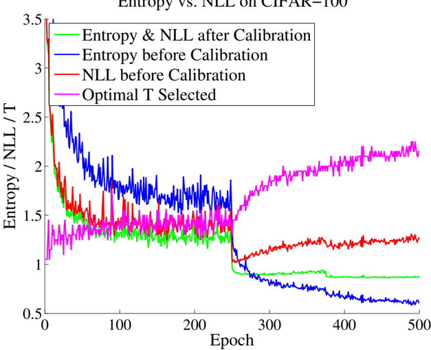Figure S1 visualizes Claim 1. We see that, as training continues, the model begins to overfit with respect to NLL (red line). This results in a low-entropy softmax distribution over classes (blue line), which explains the model's overconfidence. Temperature scaling not only lowers the NLL but also raises the entropy of the distribution (green line). ## S3. Additional Tables Tables S1, S2, and S3 display the MCE, test error, and NLL for all the experimental settings outlined in Section 5. ## Entropy vs. NLL on CIFAR-100 Figure S1. Entropy and NLL for CIFAR-100 before and after calibration. The optimal T selected by temperature scaling rises throughout optimization, as the pre-calibration entropy decreases steadily. The post-calibration entropy and NLL on the validation set coincide (which can be derived from the gradient optimality condition of T ). <details> <summary>Image 5 Details</summary>  ### Visual Description ## Line Graph: Entropy vs. NLL on CIFAR-100 ### Overview The graph illustrates the relationship between entropy, negative log-likelihood (NLL), and optimal temperature (T) across 500 training epochs on the CIFAR-100 dataset. Four data series are plotted, showing changes before and after calibration, along with the selected optimal temperature. ### Components/Axes - **X-axis (Epoch)**: Ranges from 0 to 500 in increments of 100. - **Y-axis (Entropy / NLL / T)**: Scaled from 0.5 to 3.5. - **Legend**: Located in the top-left corner, with four entries: - **Green**: Entropy & NLL after Calibration - **Blue**: Entropy before Calibration - **Red**: NLL before Calibration - **Magenta**: Optimal T Selected ### Detailed Analysis 1. **Blue Line (Entropy before Calibration)**: - Starts at ~3.5 at epoch 0, sharply declines to ~2.0 by epoch 100, then stabilizes around 1.2 by epoch 300, and further decreases to ~0.8 by epoch 500. - Trend: Steep initial drop followed by gradual stabilization. 2. **Red Line (NLL before Calibration)**: - Begins at ~3.2 at epoch 0, decreases to ~1.8 by epoch 100, stabilizes near 1.1 by epoch 300, and remains flat at ~1.0 by epoch 500. - Trend: Slightly less steep decline than the blue line, with a plateau phase. 3. **Green Line (Entropy & NLL after Calibration)**: - Starts at ~3.0 at epoch 0, drops to ~1.5 by epoch 100, stabilizes at ~1.0 by epoch 300, and remains constant at ~1.0 by epoch 500. - Trend: Sharp initial decline, then rapid stabilization. 4. **Magenta Line (Optimal T Selected)**: - Begins at ~1.2 at epoch 0, rises to ~1.5 by epoch 100, increases to ~1.8 by epoch 300, and peaks at ~2.2 by epoch 500. - Trend: Gradual upward trajectory with no plateau. ### Key Observations - **Calibration Impact**: The green line (post-calibration) consistently shows lower entropy and NLL values compared to the blue and red lines (pre-calibration), indicating improved model performance after calibration. - **Optimal T Dynamics**: The magenta line’s steady increase suggests that the optimal temperature parameter is adjusted upward over time, possibly to balance exploration and exploitation in the model. - **Stabilization**: All lines except the magenta line stabilize after ~300 epochs, implying convergence of the model’s metrics. ### Interpretation The data demonstrates that calibration significantly reduces entropy and NLL, enhancing model reliability. The Optimal T’s upward trend may reflect adaptive tuning to maintain performance as the model evolves. The stabilization of entropy and NLL post-calibration suggests that the model reaches a steady state, while the rising Optimal T indicates ongoing parameter adjustments to optimize outcomes. This aligns with techniques in machine learning where calibration and temperature scaling are used to improve generalization and confidence calibration. </details> Table S1. MCE (%) (with M = 15 bins) on standard vision and NLP datasets before calibration and with various calibration methods. The number following a model's name denotes the network depth. MCE seems very sensitive to the binning scheme and is less suited for small test sets. | Dataset | Model | Uncalibrated | Hist. Binning | Isotonic | BBQ | Temp. Scaling | Vector Scaling | Matrix Scaling | |------------------|-----------------|----------------|-----------------|------------|--------|-----------------|------------------|------------------| | Birds | ResNet 50 | 30.06% | 25.35% | 16.59% | 11.72% | 9.08% | 9.81% | 38.67% | | Cars | ResNet 50 | 41.55% | 5.16% | 15.23% | 9.31% | 20.23% | 8.59% | 29.65% | | CIFAR-10 | ResNet 110 | 33.78% | 26.87% | 7.8% | 72.64% | 8.56% | 27.39% | 22.89% | | CIFAR-10 | ResNet 110 (SD) | 34.52% | 17.0% | 16.45% | 19.26% | 15.45% | 15.55% | 10.74% | | CIFAR-10 | Wide ResNet 32 | 27.97% | 12.19% | 6.19% | 9.22% | 9.11% | 4.43% | 9.65% | | CIFAR-10 | DenseNet 40 | 22.44% | 7.77% | 19.54% | 14.57% | 4.58% | 3.17% | 4.36% | | CIFAR-10 | LeNet 5 | 8.02% | 16.49% | 18.34% | 82.35% | 5.14% | 19.39% | 16.89% | | CIFAR-100 | ResNet 110 | 35.5% | 7.03% | 10.36% | 10.9% | 4.74% | 2.5% | 45.62% | | CIFAR-100 | ResNet 110 (SD) | 26.42% | 9.12% | 10.95% | 9.12% | 8.85% | 8.85% | 35.6% | | CIFAR-100 | Wide ResNet 32 | 33.11% | 6.22% | 14.87% | 11.88% | 5.33% | 6.31% | 44.73% | | CIFAR-100 | DenseNet 40 | 21.52% | 9.36% | 10.59% | 8.67% | 19.4% | 8.82% | 38.64% | | CIFAR-100 | LeNet 5 | 10.25% | 18.61% | 3.64% | 9.96% | 5.22% | 8.65% | 18.77% | | ImageNet | DenseNet 161 | 14.07% | 13.14% | 11.57% | 10.96% | 12.29% | 9.61% | - | | ImageNet | ResNet 152 | 12.2% | 14.57% | 8.74% | 8.85% | 12.29% | 9.61% | - | | SVHN | ResNet 152 (SD) | 19.36% | 11.16% | 18.67% | 9.09% | 18.05% | 30.78% | 18.76% | | 20 News | DAN 3 | 17.03% | 10.47% | 9.13% | 6.28% | 8.21% | 8.24% | 17.43% | | Reuters | DAN 3 | 14.01% | 16.78% | 44.95% | 36.18% | 25.46% | 18.88% | 19.39% | | SST Binary | TreeLSTM | 21.66% | 3.22% | 13.91% | 36.43% | 6.03% | 6.03% | 6.03% | | SST Fine Grained | TreeLSTM | 27.85% | 28.35% | 19.0% | 8.67% | 44.75% | 11.47% | 11.78% | ## S4. 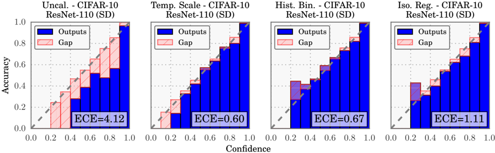Additional Reliability Diagrams We include reliability diagrams for additional datasets: CIFAR-10 (Figure S2) and SST (Figure S3 and Figure S4). Note that, as mentioned in Section 2, the reliability dia- grams do not represent the proportion of predictions that belong to a given bin. Table S2. Test error (%) on standard vision and NLP datasets before calibration and with various calibration methods. The number following a model's name denotes the network depth. Error with temperature scaling is exactly the same as uncalibrated. | Dataset | Model | Uncalibrated | Hist. Binning | Isotonic | BBQ | Temp. Scaling | Vector Scaling | Matrix Scaling | |------------------|-----------------|----------------|-----------------|------------|--------|-----------------|------------------|------------------| | Birds | ResNet 50 | 22.54% | 55.02% | 23.37% | 37.76% | 22.54% | 22.99% | 29.51% | | Cars | ResNet 50 | 14.28% | 16.24% | 14.9% | 19.25% | 14.28% | 14.15% | 17.98% | | CIFAR-10 | ResNet 110 | 6.21% | 6.45% | 6.36% | 6.25% | 6.21% | 6.37% | 6.42% | | CIFAR-10 | ResNet 110 (SD) | 5.64% | 5.59% | 5.62% | 5.55% | 5.64% | 5.62% | 5.69% | | CIFAR-10 | Wide ResNet 32 | 6.96% | 7.3% | 7.01% | 7.35% | 6.96% | 7.1% | 7.27% | | CIFAR-10 | DenseNet 40 | 5.91% | 6.12% | 5.96% | 6.0% | 5.91% | 5.96% | 6.0% | | CIFAR-10 | LeNet 5 | 15.57% | 15.63% | 15.69% | 15.64% | 15.57% | 15.53% | 15.81% | | CIFAR-100 | ResNet 110 | 27.83% | 34.78% | 28.41% | 28.56% | 27.83% | 27.82% | 38.77% | | CIFAR-100 | ResNet 110 (SD) | 24.91% | 33.78% | 25.42% | 25.17% | 24.91% | 24.99% | 35.09% | | CIFAR-100 | Wide ResNet 32 | 28.0% | 34.29% | 28.61% | 29.08% | 28.0% | 28.45% | 37.4% | | CIFAR-100 | DenseNet 40 | 26.45% | 34.78% | 26.73% | 26.4% | 26.45% | 26.25% | 36.14% | | CIFAR-100 | LeNet 5 | 44.92% | 54.06% | 45.77% | 46.82% | 44.92% | 45.53% | 52.44% | | ImageNet | DenseNet 161 | 22.57% | 48.32% | 23.2% | 47.58% | 22.57% | 22.54% | - | | ImageNet | ResNet 152 | 22.31% | 48.1% | 22.94% | 47.6% | 22.31% | 22.56% | - | | SVHN | ResNet 152 (SD) | 1.98% | 2.06% | 2.04% | 2.04% | 1.98% | 2.0% | 2.08% | | 20 News | DAN 3 | 20.06% | 25.12% | 20.29% | 20.81% | 20.06% | 19.89% | 22.0% | | Reuters | DAN 3 | 2.97% | 7.81% | 3.52% | 3.93% | 2.97% | 2.83% | 3.52% | | SST Binary | TreeLSTM | 11.81% | 12.08% | 11.75% | 11.26% | 11.81% | 11.81% | 11.81% | | SST Fine Grained | TreeLSTM | 49.5% | 49.91% | 48.55% | 49.86% | 49.5% | 49.77% | 48.51% | Table S3. NLL (%) on standard vision and NLP datasets before calibration and with various calibration methods. The number following a model's name denotes the network depth. To summarize, NLL roughly follows the trends of ECE. | Dataset | Model | Uncalibrated | Hist. Binning | Isotonic | BBQ | Temp. Scaling | Vector Scaling | Matrix Scaling | |------------------|-----------------|----------------|-----------------|------------|--------|-----------------|------------------|------------------| | Birds | ResNet 50 | 0.9786 | 1.6226 | 1.4128 | 1.2539 | 0.8792 | 0.9021 | 2.334 | | Cars | ResNet 50 | 0.5488 | 0.7977 | 0.8793 | 0.6986 | 0.5311 | 0.5299 | 1.0206 | | CIFAR-10 | ResNet 110 | 0.3285 | 0.2532 | 0.2237 | 0.263 | 0.2102 | 0.2088 | 0.2048 | | CIFAR-10 | ResNet 110 (SD) | 0.2959 | 0.2027 | 0.1867 | 0.2159 | 0.1718 | 0.1709 | 0.1766 | | CIFAR-10 | Wide ResNet 32 | 0.3293 | 0.2778 | 0.2428 | 0.2774 | 0.2283 | 0.2275 | 0.2229 | | CIFAR-10 | DenseNet 40 | 0.2228 | 0.212 | 0.1969 | 0.2087 | 0.175 | 0.1757 | 0.176 | | CIFAR-10 | LeNet 5 | 0.4688 | 0.529 | 0.4757 | 0.4984 | 0.459 | 0.4568 | 0.4607 | | CIFAR-100 | ResNet 110 | 1.4978 | 1.4379 | 1.207 | 1.5466 | 1.0442 | 1.0485 | 2.5637 | | CIFAR-100 | ResNet 110 (SD) | 1.1157 | 1.1985 | 1.0317 | 1.1982 | 0.8613 | 0.8655 | 1.8182 | | CIFAR-100 | Wide ResNet 32 | 1.3434 | 1.4499 | 1.2086 | 1.459 | 1.0565 | 1.0648 | 2.5507 | | CIFAR-100 | DenseNet 40 | 1.0134 | 1.2156 | 1.0615 | 1.1572 | 0.9026 | 0.9011 | 1.9639 | | CIFAR-100 | LeNet 5 | 1.6639 | 2.2574 | 1.8173 | 1.9893 | 1.656 | 1.6648 | 2.1405 | | ImageNet | DenseNet 161 | 0.9338 | 1.4716 | 1.1912 | 1.4272 | 0.8885 | 0.8879 | - | | ImageNet | ResNet 152 | 0.8961 | 1.4507 | 1.1859 | 1.3987 | 0.8657 | 0.8742 | - | | SVHN | ResNet 152 (SD) | 0.0842 | 0.1137 | 0.095 | 0.1062 | 0.0821 | 0.0844 | 0.0924 | | 20 News | DAN 3 | 0.7949 | 1.0499 | 0.8968 | 0.9519 | 0.7387 | 0.7296 | 0.9089 | | Reuters | DAN 3 | 0.102 | 0.2403 | 0.1475 | 0.1167 | 0.0994 | 0.099 | 0.1491 | | SST Binary | TreeLSTM | 0.3367 | 0.2842 | 0.2908 | 0.2778 | 0.2739 | 0.2739 | 0.2739 | | SST Fine Grained | TreeLSTM | 1.1475 | 1.1717 | 1.1661 | 1.149 | 1.1168 | 1.1085 | 1.1112 | <details> <summary>Image 6 Details</summary>  ### Visual Description ## Bar Charts: Calibration Methods on CIFAR-10 with ResNet-110 (SD) ### Overview The image contains four side-by-side bar charts comparing calibration performance of different methods on the CIFAR-10 dataset using ResNet-110 (SD). Each chart visualizes the relationship between model confidence intervals and accuracy, with Expected Calibration Error (ECE) values provided for each method. ### Components/Axes - **X-axis**: "Confidence" (0.0 to 1.0 in 0.2 increments) - **Y-axis**: "Accuracy" (0.0 to 1.0 in 0.2 increments) - **Legend**: - Blue bars: "Outputs" (model's predicted accuracy at confidence intervals) - Pink bars: "Gap" (difference between confidence and accuracy) - **Chart Titles**: 1. Uncal. - CIFAR-10 ResNet-110 (SD) 2. Temp. Scale - CIFAR-10 ResNet-110 (SD) 3. Hist. Bin. - CIFAR-10 ResNet-110 (SD) 4. Iso. Reg. - CIFAR-10 ResNet-110 (SD) ### Detailed Analysis 1. **Uncal. (Uncalibrated)** - ECE = 4.12 (highest error) - "Outputs" bars show significant gaps between confidence and accuracy, especially at lower confidence intervals (0.0–0.4) - "Gap" bars are large and irregular, indicating poor calibration 2. **Temp. Scale (Temperature Scaling)** - ECE = 0.60 - "Outputs" bars show gradual improvement in calibration across confidence intervals - "Gap" bars are smaller and more consistent than Uncal., but still show moderate discrepancies 3. **Hist. Bin. (Histogram Binning)** - ECE = 0.67 - "Outputs" bars demonstrate the most consistent calibration, with minimal gaps across confidence intervals - "Gap" bars are smallest among all methods, indicating optimal calibration 4. **Iso. Reg. (Isotonic Regression)** - ECE = 1.11 (highest error among calibrated methods) - "Outputs" bars show erratic calibration, with large gaps at mid-to-high confidence intervals (0.4–1.0) - "Gap" bars are largest at higher confidence levels, suggesting overconfidence ### Key Observations - **ECE Trends**: Hist. Bin. (0.67) < Temp. Scale (0.60) < Iso. Reg. (1.11) < Uncal. (4.12) - **Calibration Effectiveness**: Hist. Bin. achieves the lowest ECE, demonstrating superior calibration. Uncal. performs worst due to lack of calibration. - **Gap Patterns**: Larger "Gap" bars in Uncal. and Iso. Reg. indicate systematic over/underconfidence. Hist. Bin. shows the most balanced confidence-accuracy alignment. ### Interpretation The data reveals that calibration methods significantly impact model reliability. Histogram binning (Hist. Bin.) achieves the most accurate confidence estimates (lowest ECE), while uncalibrated models (Uncal.) exhibit extreme calibration errors. Temperature scaling (Temp. Scale) provides moderate improvement, but isotonic regression (Iso. Reg.) paradoxically performs worse than uncalibrated models in this context. The "Gap" visualization highlights that calibration reduces but does not eliminate confidence-accuracy mismatches, with Hist. Bin. achieving the most balanced performance. These results emphasize the importance of calibration in safety-critical applications where reliable confidence estimates are essential. </details> Figure S2. Reliability diagrams for CIFAR-10 before (far left) and after calibration (middle left, middle right, far right). Figure S3. Reliability diagrams for SST Binary and SST Fine Grained before (far left) and after calibration (middle left, middle right, far right). 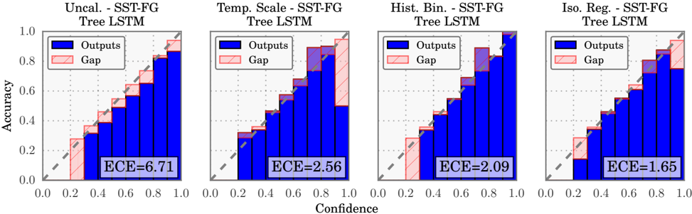<details> <summary>Image 7 Details</summary>  ### Visual Description ## BarChart: Tree LSTM Model Performance Across Configurations ### Overview The image displays four side-by-side bar charts comparing the performance of a Tree LSTM model under different configurations. Each chart evaluates the relationship between **confidence** (x-axis) and **accuracy** (y-axis), with two data series: **Outputs** (blue bars) and **Gap** (pink bars). The charts are labeled with configuration names and include Expected Calibration Error (ECE) values. --- ### Components/Axes - **X-axis**: "Confidence" (ranges from 0.0 to 1.0 in 0.2 increments). - **Y-axis**: "Accuracy" (ranges from 0.0 to 1.0 in 0.2 increments). - **Legend**: - Blue bars: "Outputs" (model's predicted accuracy). - Pink bars: "Gap" (difference between confidence and accuracy). - **ECE Values**: Annotated in the bottom-left corner of each chart (e.g., ECE=6.71, ECE=2.56, etc.). --- ### Detailed Analysis 1. **Uncal. - SST-FG Tree LSTM** (ECE=6.71): - **Outputs**: Accuracy increases with confidence, peaking at ~0.85 for confidence >0.8. - **Gap**: Consistently smaller than Outputs, with a maximum gap of ~0.15 at confidence=1.0. - **Trend**: Outputs show a stepwise increase, while the gap narrows as confidence grows. 2. **Temp. Scale - SST-FG Tree LSTM** (ECE=2.56): - **Outputs**: Smoother upward trend compared to Uncal., reaching ~0.9 at confidence=1.0. - **Gap**: Smaller than Uncal., with a maximum gap of ~0.1 at confidence=1.0. - **Trend**: Outputs and gap both improve, indicating better calibration. 3. **Hist. Bin. - SST-FG Tree LSTM** (ECE=2.09): - **Outputs**: Similar trend to Temp. Scale but with slightly lower accuracy (~0.85 at confidence=1.0). - **Gap**: Narrower than Temp. Scale, with a maximum gap of ~0.08. - **Trend**: Improved calibration over previous configurations. 4. **Iso. Reg. - SST-FG Tree LSTM** (ECE=1.65): - **Outputs**: Highest accuracy (~0.95 at confidence=1.0). - **Gap**: Smallest gap (~0.05 at confidence=1.0). - **Trend**: Outputs and gap both show minimal deviation, indicating optimal calibration. --- ### Key Observations - **ECE Decrease**: ECE values decrease from left to right (6.71 → 1.65), suggesting improved calibration with more sophisticated configurations. - **Gap Reduction**: The "Gap" bars shrink significantly in later configurations, indicating reduced discrepancy between confidence and accuracy. - **Outputs Trend**: All configurations show increasing accuracy with confidence, but Iso. Reg. achieves the highest performance. --- ### Interpretation The data demonstrates that the Tree LSTM model's performance improves with advanced configurations (e.g., Iso. Reg.). Lower ECE values correlate with better calibration, meaning the model's confidence aligns more closely with actual accuracy. The "Gap" metric highlights that earlier configurations overestimate confidence, while later ones achieve near-optimal calibration. This suggests that techniques like temperature scaling, histogram binning, and isolation regularization enhance the model's reliability, making it more trustworthy for high-stakes applications. </details> Figure S4. Reliability diagrams for SST Binary and SST Fine Grained before (far left) and after calibration (middle left, middle right, far right). 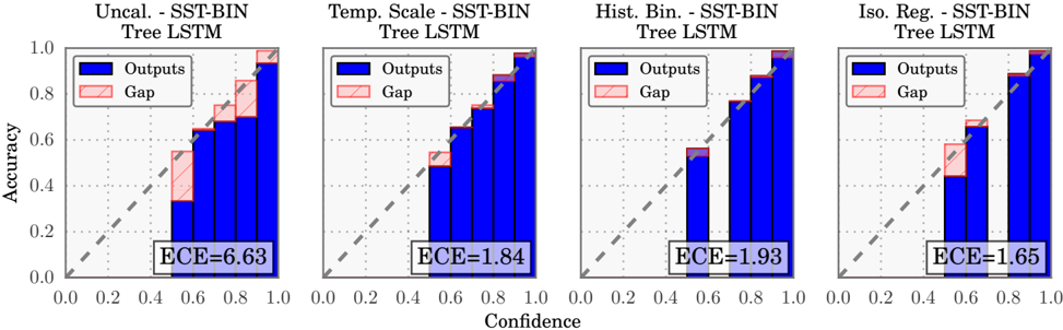<details> <summary>Image 8 Details</summary>  ### Visual Description ## Bar Chart: Model Calibration Performance Comparison ### Overview The image contains four grouped bar charts comparing calibration performance metrics (accuracy, confidence, Expected Calibration Error) across four model configurations: Uncalibrated, Temperature Scaling, Histogram Binning, and Isotonic Regression. Each chart uses a dual-color bar system (blue for "Outputs", pink for "Gap") to visualize the relationship between confidence intervals and accuracy. ### Components/Axes - **X-axis**: Confidence (0.0 to 1.0 in 0.2 increments) - **Y-axis**: Accuracy (0.0 to 1.0 in 0.2 increments) - **Legend**: - Blue = Outputs (model confidence) - Pink = Gap (difference between confidence and accuracy) - **Subplots**: 1. Uncal. - SST-BIN Tree LSTM 2. Temp. Scale - SST-BIN Tree LSTM 3. Hist. Bin. - SST-BIN Tree LSTM 4. Iso. Reg. - SST-BIN Tree LSTM - **Annotations**: - Diagonal dashed line (perfect calibration reference) - ECE values in bottom-left corner of each subplot ### Detailed Analysis 1. **Uncal. - SST-BIN Tree LSTM** - ECE = 6.63 (highest error) - Blue bars show increasing accuracy with confidence - Pink gaps decrease slightly with higher confidence intervals - Largest discrepancy between confidence and accuracy at 0.0-0.2 confidence range 2. **Temp. Scale - SST-BIN Tree LSTM** - ECE = 1.84 - Blue bars show steeper accuracy increase - Pink gaps remain relatively consistent across confidence intervals - Better alignment between confidence and accuracy than Uncal. model 3. **Hist. Bin. - SST-BIN Tree LSTM** - ECE = 1.93 - Blue bars show moderate accuracy growth - Pink gaps decrease significantly at higher confidence intervals - Largest calibration error at 0.0-0.2 confidence range 4. **Iso. Reg. - SST-BIN Tree LSTM** - ECE = 1.65 (lowest error) - Blue bars show gradual accuracy increase - Pink gaps decrease proportionally with confidence - Most consistent calibration across all confidence intervals ### Key Observations - All models show increasing accuracy with higher confidence intervals - Calibration error (ECE) decreases significantly from Uncalibrated (6.63) to Isotonic Regression (1.65) - Isotonic Regression demonstrates the smallest gap between confidence and accuracy across all intervals - Histogram Binning shows the most dramatic reduction in calibration gap at higher confidence levels - Temperature Scaling maintains relatively consistent calibration gaps across confidence intervals ### Interpretation The data demonstrates that model calibration significantly impacts performance reliability. Isotonic Regression achieves the best calibration (lowest ECE=1.65), indicating its confidence predictions most accurately reflect true accuracy. The Uncalibrated model's high ECE (6.63) suggests severe overconfidence in low-confidence predictions. The consistent decrease in calibration gaps across confidence intervals in all models suggests that higher confidence predictions are generally more reliable, but calibration techniques (particularly Isotonic Regression) are critical for maintaining this relationship across the full confidence spectrum. The pink "Gap" bars visually quantify the calibration error magnitude at each confidence level, with smaller gaps indicating better model reliability. </details>