1706.05261

## From Propositional Logic to Plausible Reasoning: A Uniqueness Theorem Kevin S. Van Horn Adobe Systems, 3900 Adobe Way, Lehi, UT 84043, United States ## Abstract We consider the question of extending propositional logic to a logic of plausible reasoning, and posit four requirements that any such extension should satisfy. Each is a requirement that some property of classical propositional logic be preserved in the extended logic; as such, the requirements are simpler and less problematic than those used in Cox's Theorem and its variants. As with Cox's Theorem, our requirements imply that the extended logic must be isomorphic to (finite-set) probability theory. We also obtain specific numerical values for the probabilities, recovering the classical definition of probability as a theorem , with truth assignments that satisfy the premise playing the role of the 'possible cases.' Keywords: Bayesian, Carnap, Cox, Jaynes, logic, probability ## 1. Introduction E. T. Jaynes [13, p. xxii] proposes the view that probability theory is the uniquely determined extension of classical propositional logic (CPL) to a 'logic of plausible reasoning' : Our theme is simply: probability theory as extended logic . . . . the mathematical rules of probability theory are not merely rules for calculating frequencies of 'random variables'; they are also the unique consistent rules for conducting inference (i.e. plausible reasoning) of any kind. . . This view is grounded in the work of Pólya [17] and Cox [9], especially the latter. In this paper we aim to set the notion of probability theory as the necessary extension of CPL on solid footing. I Submitted and currently under review at International Journal of Approximate Reasoning . II c © 2017. This manuscript version is made available under the CC-BY-NC-ND 4.0 license . http://creativecommons.org/licenses/by-nc-nd/4.0/ Email address: vanhorn@adobe.com (Kevin S. Van Horn) Our goal is to generalize the logical consequence relation, which deals only in certitudes, to handle degrees of certainty. Whereas X | = A means that A (the conclusion) is a logical consequence of X (the premise), we write A | X for 'the reasonable credibility of the proposition A (the query) when the proposition X (the premise) is known to be true' (paraphrasing Cox [9].) We call ( · | · ) the plausibility function . If X | = A then A | X is some value indicating 'certainly true,' if X | = ¬ A then A | X is some value indicating 'certainly false,' and otherwise A | X is a value indicating some intermediate level of plausibility. Our task is to determine what the plausibility function must be, based on logical criteria. As a generalization of the logical consequence relation, the plausibility function must depend only on its two explicit arguments; the value it returns must not depend on any additional information that varies according to the problem domain to which it is applied, nor according to the intended meanings of the propositional symbols. This is a formal logical theory we are developing, and so any intended semantics of the propositional symbols must be expressed axiomatically in the premise. One might question whether all relevant information for determining the plausibility of some proposition A can be expressed in propositional form for inclusion in the premise X . Might not our background information include 'soft' relationships, mere propensities for propositions to be associated in some way? Although we provide some suggestive examples, we do not attempt to resolve that question. Instead we ask, given that the background information and intended semantics are expressed in propositional form and included in the premise, with no other information available, what can we conclude about the plausibility function? We posit four Requirements for the plausibility function. Each of these requires that some property of the logical consequence relation be retained in the generalization to a plausibility function. Three are invariance properties, and the fourth is a requirement to preserve distinctions in degree of plausibility that already exist within CPL. These Requirements (discussed in detail later) are the following: - R1. If X and Y are logically equivalent, and A and B are logically equivalent assuming X , then A | X = B | Y (Section 4.) - R2. We may define a new propositional symbol without affecting the plausibility of any proposition that does not mention that symbol. Specifically, if s is a propositional symbol not appearing in A , X , or E , then A | X = A | ( s ↔ E ) ∧ X (Section 5.) - R3. Adding irrelevant information to the premise does not affect the plausibility of the query. Specifically, if Y is a satisfiable propositional formula that uses no propositional symbol occurring in A or X , then A | X = A | Y ∧ X (Section 6.) - R4. The implication ordering is preserved: if X | = A → B but not X | = B → A then A | X is a plausibility value that is strictly less than B | X (Section 7.) Note that we do not assume that plausibility values are real numbers, nor that they are totally ordered; R4 presumes only that there is some partial order on plausibility values. Given R1-R4, we prove that plausibilities are essentially probabilities in disguise. Specifically, we show that 1. there is an order-preserving isomorphism P between the set of plausibility values P and the set of rational probabilities Q ∩ [0 , 1] ; 2. P ( A | X ) , the plausibility A | X mapped via P to the unit interval, is necessarily the ratio of the number of truth assignments that satisfy both A and X to the number of truth assignments that satisfy X ; and 3. hence the usual laws of probability follow as a consequence. This identifies finite-set probability theory as the uniquely determined extension of CPL to a logic of plausible reasoning. The body of this paper is organized as follows: - In Section 2 we compare this work to Cox's Theorem and variants, as well as Carnap's system of logical probability. - In Section 3 we review some notions from CPL, discuss the partial plausibility ordering that already exists within CPL, and discuss the nature of the plausibility function. - Our main result is proven in Sections 4, 5, 6, and 7, which also introduce the Requirements, discuss the motivation behind them, and explore some of their consequences. Along the way we discuss how Carnap's system violates R3. - In Section 8 we prove that R1-R4 are consistent. - Section 9 discusses three topics: the connection of our results to the classical definition of probability, the issue of non-uniform probabilities, and an initial attempt at extending our results to infinite domains. ## 2. Relation to Prior Work To set the context for this paper, clarify our goals, and head off possible misconceptions, we now review similar prior work and point out the differences. ## 2.1. Cox's Theorem R. T. Cox [9] proposes a handful of intuitively-appealing, qualitative requirements for any system of plausible reasoning, and shows that these requirements imply that any such system is just probability theory in disguise. Specifically, he shows that there is an order isomorphism between plausibilities and the unit interval [0 , 1] such that A | X , after mapping from plausibilities to [0 , 1] , respects the laws of probability. Over the years Cox's arguments have been refined by others [1, 13, 16, 20, 21], making explicit some requirements that were only implicit in Cox's original presentation, and replacing some of the requirements with slightly less demanding assumptions than those used in Cox's original proof. One version of the requirements [21] may be summarized as follows: C1. A | X is a real number. - C2. A | X = A ′ | X whenever A is logically equivalent to A ′ , and B | X ≤ A | X for any tautology A . - C3. There exists a nonincreasing function S such that ¬ A | X = S ( A | X ) for all A and satisfiable X . - C4. The set of plausibility triples ( y 1 , y 2 , y 3 ) where y 1 = A 1 | X , y 2 = A 2 | A 1 ∧ X , and y 3 = A 3 | A 2 ∧ A 1 ∧ X for some A 1 , A 2 , A 3 , and X , is dense in [0 , 1] 3 . - C5. There exists a continuous function F : [ f , t ] 2 → [ f , t ] , strictly increasing in both arguments on ( f , t ] 2 , such that A ∧ B | X = F ( A | B ∧ X, B | X ) for any A , B , and satisfiable X . Here we use t A | X for any tautology A , and f S ( t ) . These requirements have not been without controversy. For example, Shafer [18] objects to C1, C3, and C5; Halpern [11, 12] questions C4; and Colyvan [8] objects to C2 on the basis that it presumes the law of the excluded middle. Our approach has no equivalent of C1, C3, C4, or C5: - We are agnostic as to the set of allowed plausibility values. We do not even require that plausibility values be totally ordered. - We have no requirement on how the plausibility ¬ A decomposes. - We have no density requirement on plausibility values. - We have no requirement on how the plausibility of A ∧ B decomposes, much less any continuity or strictness requirements for such decompositions. We do retain a variant of C2. Our goal is to extend the classical propositional logic; we make no attempt to address intuitionistic logic. Our requirements are all based on preserving in the extended logic some existing property of CPL. Three of these are invariances-ways in which A or X may be modified without altering A | X -and the last is a requirement to preserve those distinctions in degree of plausibility already present in CPL. We believe that such an approach leaves far less room for objections to the requirements. The results we obtain are similar to those of Cox's Theorem, with these differences: - Weobtain an order isomorphism P between plausibility values and rational probability values. - We obtain specific numerical values for P ( A | X ) , and not just the laws for decomposing P ( A | X ) . - The conditioning information X is necessarily a propositional formula. (Some variants [7, 13, 21] of Cox's Theorem allow X to be an undefined 'state of information' to which we may add additional propositional information.) - Our results apply only to finite problem domains or finite approximations of infinite domains. (In Section 9.3 we discuss how to extend our results to infinite domains.) ## 2.2. Clayton and Waddington: bridging the intution gap In a recent paper, Clayton and Waddington [7] seek to 'bridge the intuition gap' in Cox's Theorem by proposing alternative requirements they argue are more intuitively reasonable, and then proving C4 and the strictness of F in C5 as theorems. We find their most interesting and important contributions to be the following: - Rather than just tweaking Cox's Theorem, they have instead created an entirely new proof of its result. The meat of the proof of Cox's Theorem lies in deriving functional equations that F and S must satisfy, then solving those equations. But by the time they have 'bridged the intuition gap' in the requirements, they already have most of the proof completed, without any need to solve functional equations. - Jaynes [13] argues that, if one's background information is 'indifferent' between two propositions, then they should be assigned equal plausibility. They formalize this idea as an invariance principle: if A ′ | X ′ is obtained from A | X by consistently renaming all propositional symbols used via a one-to-one mapping, then the two plausibilities are equal. - Their proof yields the classical definition of probability-the ratio of the number of positive cases to the number of all possible cases-as a theorem in certain cases they call ' N -urns.' However, the list of assumptions they use is fairly long: 11 altogether. We obtain similar results with fewer and simpler requirements, given in Sections 4-7. Here is a comparison: - Clayton and Waddington use a variant of C2 that replaces ' A is logically equivalent to A ′ ' with ' A ∧ X is logically equivalent to A ′ ∧ X '; this and their Assumption 2.1 are comparable to our R1 (replacement of premise or query with a logically equivalent formula). - Our R4 (preservation of the implication ordering) is a stronger (more general) version of their Assumption 2.7. We do not actually need this more general form-Lemma 13 only uses a restricted form that corresponds to their Assumption 2.7-but we feel that the rationale for the requirement is more clearly seen in this more general form. - Our R2 (invariance under definition of new propositional symbols) and R3 (invariance under addition of irrelevant information) have no direct equivalent among their assumptions, but are inspired by their discussion of the Principle of Indifference and their Assumption 2.3 (translation invariance). - We use no equivalent of C1 nor their Assumptions 1.2, 1.3, 1.4, 3.2, 3.3, and 3.5. From the above comparison one can see that it is the replacement of Assumption 2.3 with R2 and R3 that allows a drastic pruning of the assumptions used in obtaining the main results of their paper. Our approach was inspired by Clayton and Waddington's notion of an ' N -urn' and the results they prove for N -urns. Our most important innovation is Lemma 6 showing how to reduce every allowable query-premise pair to a certain kind of N -urn. ## 2.3. Carnap: logical probability Carnap [5] undertakes an extensive investigation of 'logical probability.' He mentions two notions of probability: probability 1 is epistemic probability 1 ('the degree of confirmation of a hypothesis h with respect to an evidence statement e '), and probability 2 is relative frequency. His focus is on probability 1 and the problem of induction. Our terminology and his correspond roughly as follows: - Instead of a 'plausibility function' Carnap discusses a 'confirmation function' c . - The rough equivalent of A | X in Carnap's system is c ( A,X ) , with a crucial difference described below. - We call A and X the query and premise, respectively; he calls them the hypothesis and evidence. We take A and X to be propositional formulas, whereas Carnap allows them to be sentences in a variant of first-order predicate logic in which the only allowed terms are variables and constant symbols. The domain of discourse is taken to be a countably infinite set of individuals, and for each individual there is a corresponding constant symbol. He calls this most general form of the language L ∞ . 1 Carnap later favored a decision-theoretic view of probability 1 [5, Preface to the Second Edition]. Carnap also considers restricted languages L N , N ≥ 1 , in which only the first N constant symbols are allowed and the domain of discourse is only the first N individuals. Most of the focus is on the finite languages L N , with confirmation functions for L ∞ defined via a limiting process on the sequence of languages L N , N ≥ 1 . This is similar in spirit, though not in detail, to our approach to infinite domains. A difference between Carnap's approach and ours is that we posit a single language and single set of propositional symbols S to be used for all problem domains, whereas in Carnap's system each problem domain has its own language L ∞ with its own set of predicate symbols and associated arities and interpretations. Carnap's finite languages L N are equivalent to propositional languages with a finite number of propositional symbols. Let an atomic sentence be a formula of the form p ( s 1 , . . . , s k ) for some k -ary predicate symbol p and constant symbols s 1 , . . . , s k . There are a finite number of distinct atomic sentences in L N . Define the propositional language L ′ N to have as propositional symbols the atomic sentences of L N . We can transform any sentence A ∈ L N into an equivalent propositional formula A ′ ∈ L ′ N : 1. Remove all quantifiers by repeatedly replacing any occurrence of a subformula ∀ xϕ ( x ) with the semantically equivalent finite conjunction ϕ ( s 1 ) ∧ · · · ∧ ϕ ( s N ) , where s 1 , . . . , s N are the constant symbols for the first N individuals. 2. If equality is allowed, replace any subformula s i = s i with a logically valid sentence, and any subformula s i = s j , i = j , with an unsatisfiable sentence. In both cases choose replacement sentences that contain no quantifiers nor use of equality. (Carnap specifies that distinct constant symbols are assumed to reference distinct individuals.) We end up with propositional formulas in which the propositional symbols have internal structure, but this internal structure is of no consequence from the standpoint of deductive logic. To have logical effect, any intended meaning for this internal structure must be given by additional formulas in L ′ N , axioms that are added to the set of premises used. For example, suppose that we are deducing the logical consequences of a set of premises Γ , that we have a twoplace predicate lt , and that the intended meaning of lt( x, y ) is that individual x precedes individuals y in some total ordering. Then we must add to Γ a set of axioms such as the following: $$\begin{array} { c } \forall x \, \neg l t ( x , x ) \\ \forall x \, \forall y \, \left ( l t ( x , y ) \vee l t ( y , x ) \vee x = y \right ) \\ \forall x \, \forall y \, \forall z \, \left ( l t ( x , y ) \land l t ( y , z ) \rightarrow l t ( x , z ) \right ) \end{array}$$ More precisely, we must add to Γ the result of transforming the above sentences of L N into equivalent propositional formulas of L ′ N . Carnap, however, is unwilling to axiomatize the intended interpretations of the predicate symbols in this way. He writes [5, p. 55], Since we intend to construct inductive logic as a theory of degree of confirmation, based upon the meanings of the sentences involvedin contradistinction to a mere calculus -we shall construct the language systems L with an interpretation, hence as a system of semantical rules, not as uninterpreted syntactical systems. (Emphasis added.) This is an important difference between Carnap's system and ours, one that we discuss further in Section 3.4 and Section 9.2. Thus the equivalent of Carnap's c ( h, e ) in our scheme is not h | e , but instead h | e ∧ X , where X is a conjunction of - propositional axioms expressing the logical structure of the problem domain, and - propositional formulas expressing any other background information. Unlike Cox [9], Carnap makes no attempt to derive the laws of probability from more fundamental considerations; instead, his 'conventions on adequacy' [5, p. 285] require that a valid confirmation function should conform to the laws of probability. He ensures this by proceeding as follows: 1. A state description for L N amounts to a truth assignment on the set of atomic sentences of L N . 2. A regular measure function for L N amounts to a strictly positive probability mass function over the set of state descriptions for L N . 3. A regular confirmation function c for L N is then a confirmation function defined as $$c ( h , e ) = m ( h \wedge e ) / m ( e )$$ for some regular measure function m on L N . 4. These notions are extended to L ∞ by imposing a consistency condition on a sequence of regular measure functions m N on L N , N ≥ 1 , considering the associated regular confirmation functions c N , and defining c ∞ ( h, e ) = lim N →∞ c N ( h, e ) . We see therefore that, although it is the conditional probabilities c ( h, e ) that most interest Carnap, unconditional probabilities are for him more fundamental. In contrast, we take conditional plausibilities as the fundamental concept and, rather than imposing the laws of probability, seek to derive them. Carnap's goal is that the confirmation function appropriate to a problem domain should be uniquely determined by the semantics of the language L ∞ , specifically, the intended interpretation of the predicate symbols and constant symbols. In this he fails. Limiting his attention to systems that contain monadic predicates ('properties') only, he proposes a specific confirmation function c ∗ , but says [5, p. 563], Now the chief arguments in favor of the function c ∗ . . . will consist in showing that this function is free of the inadequacies in the other methods. It may then still be inadequate in other respects. It will not be claimed that c ∗ is a perfectly adequate explicatum for probability 1 , let alone that it is the only adequate one. . . He later [5, Preface to Second Edition][6] proposes instead an entire family of confirmation functions c λ parameterized by a positive number λ . In contrast, we show in Theorem 14 that there is (up to isomorphism) a single , unique plausibility function satisfying our criteria. Ironically, it corresponds to the one confirmation function explicitly rejected by Carnap: a uniform distribution over the set of truth assignments satisfying the premise / evidence. We discuss this further in Section 9.2. ## 3. Logical Preliminaries In this section we review some concepts from CPL, introduce some additional logical concepts of our own, and discuss the nature of the plausibility function as extending the logical consequence relation | = . ## 3.1. Review of classical propositional logic A proposition is a statement or assertion that must be true or false; it is atomic if it cannot be decomposed into simpler assertions. A propositional symbol is one of a countably infinite set of symbols S that are used to represent atomic propositions. We abbreviate this to just 'symbol' when the meaning is clear. If S ⊆ S then a propositional formula on S is one of the following: - a propositional symbol from S ; - a formula ¬ A , meaning 'not A ', for some propositional formula A on S ; or - a formula A ∧ B , meaning ' A and B ,' where A and B are propositional formulas on S . The other common logical operatorsA ∨ B (or), A → B (implies), and A ↔ B (if and only if)-are defined in terms of ¬ and ∧ in the usual way. We abbreviate 'propositional formula' as just 'formula' when the meaning is clear. We write Φ( S ) for the set of all propositional formulas on S , and Φ + ( S ) for the satisfiable formulas. We write σ J A 1 , . . . , A n K for the set of all propositional symbols occuring in any of the propositional formulas A 1 , . . . , A n . A truth assignment on S is a function ρ : S →{ 0 , 1 } , with 0 and 1 standing for falsity and truth, respectively. We recursively extend it to all formulas on S in the obvious way: $$</text> \begin{array} { r l r } { \rho [ A ] } & = } & { \rho ( A ) i f A \in S } \\ { \rho [ \neg A ] } & = } & { 1 - \rho [ A ] } \\ { \rho [ A \land B ] } & = } & { \rho [ A ] \cdot \rho [ B ] } \end{array}$$ where ' · ' is just integer multiplication. A truth assignment ρ on S satisfies a formula A on S if ρ J A K = 1 . A formula A is satisfiable if there is some truth assignment ρ on σ J A K that satisfies A . A formula A is logically valid , written | = A , if every truth assignment on σ J A K satisfies A . We say that B is a logical consequence of A , or A logically implies B , written A | = B , if every truth assignment on σ J A,B K that satisfies A also satisfies B . This captures the notion of a logically valid argument: conclusion B follows as a logical consequence of premises A 1 , . . . , A n if A 1 ∧ · · · ∧ A n | = B . Note that A | = B if and only if | = A → B . The restriction of a truth assignment ρ on S to some S ′ ⊆ S is the truth assignment ρ ′ on S ′ such that ρ ′ ( s ) = ρ ( s ) for every s ∈ S ′ . Note that ρ J A K depends only on the truth values assigned to those symbols that actually appear in A ; if A is a formula on S ′ ⊆ S , ρ is a truth assignment on S , and ρ ′ is the restriction of ρ to S ′ , then ρ ′ J A K = ρ J A K . Because of this, we have some leeway in choosing the set of propositional symbols to use in the definitions of 'logically valid,' 'satisfiable,' and 'logical consequence.' If σ J A K ⊆ S A and σ J A,B K ⊆ S AB , then - A is logically valid iff every truth assignment on S A satisfies A . - A is satisfiable iff some truth assignment on S A satisfies A . - A | = B iff every truth assignment on S AB that satisfies A also satisfies B . ## Some notation. - Two formulas are logically equivalent , written A ≡ B , if | = A ↔ B . - A and B are logically equivalent assuming X , written A ≡ X B , if X | = A ↔ B . - We will use finite quantification as an abbreviation where convenient, for example writing ∧ n i =1 A i for A 1 ∧ · · · ∧ A n . - If we write A 1 ∧ · · · ∧ A n and n = 0 , we understand this to mean some logically valid formula such as s ∨ ¬ s . - If we write A 1 ∨ · · · ∨ A n and n = 0 , we understand this to mean some unsatisfiable formula such as s ∧ ¬ s . ## 3.2. Finite sample spaces The development of probability theory usually begins with the idea of a sample space, which has been downplayed so far-the focus has been on propositions. We find in Theorem 14 that A | X can be characterized in terms of an induced sample space: the set of truth assignments that satisfy X . 2 In particular, we find that A | X is a function of the proportion of points from this induced sample space that satisfy A . This motivates the following: 2 This is similar to Carnap's system, in which the set of state descriptions serve as a sample space. Definition 1. # S ( X ) is the number of truth assignments on S satisfying X , for any formula X and finite S such that σ J X K ⊆ S ⊆ S . The size of the induced sample space is # S ( X ) , and the proportion of points from the induced sample space that satisfy A is # S ( A ∧ X ) / # S ( X ) , for S ⊇ σ A,X . J K Typically one thinks of a finite sample space as an arbitrary set of n > 0 distinct values Ω = { ω 1 , . . . , ω n } representing different possible states of some system under consideration. We can relate this to our notion of an induced sample space by choosing a set of n propositional symbols S = { s 1 , . . . , s n } , with the intended interpretation of s i being that the state of the system is ω i . If our premise X is a formula expressing that exactly one of the s i is true, then there is a one-to-one correspondence between our original sample space Ω and the induced sample space of truth assignments, with ω i corresponding to the single truth assignment ρ on S satisfying s i ∧ X . This motivates the following: Definition 2. Given any sequence of n > 0 propositional symbols s 1 , . . . , s n , $$\langle s _ { 1 } , \dots , s _ { n } \rangle = ( s _ { 1 } \vee \cdots \vee s _ { n } ) \wedge \bigwedge _ { 1 \leq i < j \leq n } \neg ( s _ { i } \wedge s _ { j } ) \, ;$$ that is, 〈 s 1 , . . . , s n 〉 means that exactly one of the s i is true. ## 3.3. The implication ordering At first blush it would seem that CPL tells us very little about the relative plausibilities of different propositions, beyond determining which are certainly true and which are certainly false given a premise X . The reality is quite the opposite: CPL comes equipped with a rich inherent plausibility ordering that we call the implication ordering . Definition 3. Let A,B,X ∈ Φ( S ) with X satisfiable. We define $$( A \preceq _ { x } B ) \quad \Leftrightarrow \quad ( X \models A \rightarrow B )$$ $$\begin{array} { r l } { ( A \prec _ { x } B ) } & \Leftrightarrow } & { ( A \preceq _ { x } B ) a n d n o t } & { ( B \preceq _ { x } A ) \, . } \end{array}$$ $$a n d n o t \, ( B \preceq _ { x } A ) \, .$$ The following properties are easily verified: - The relation X is a preorder: it is reflexive and transitive, but not antisymmetric. - A ≺ X B is the same as ( A X B and not A ≡ X B ). - A ≡ X B if and only A X B and B X A . - If A ≡ X A ′ and B ≡ X B ′ and A X B then A ′ X B ′ . Hence X defines a partial order on the equivalence classes of propositional formulas under the relation ≡ X . This partial order is essentially just the subset ordering on truth assignments: Property. Let A 1 , A 2 , X ∈ Φ( S ) with X satisfiable. Then A 1 X A 2 if and only if α J A 1 K ⊆ α J A 2 K , where α J A K is the set of truth assignments on S that satisfy both A and X . Assuming X , we therefore conclude the following: - If A X B then B is at least as plausible as A , since B is true for any possible world (truth assignment satisfying X ) for which A is true. - If A ≡ X B then A X B and B X A , hence A and B are equally plausible. - If A ≺ X B then B is strictly more plausible than A , since there are possible worlds for which B is true and A is not, but not vice versa. Consider an example that uses three propositional symbols s 1 , s 2 , s 3 with X defined to be the formula stating that exactly one of these three is true: X = 〈 s 1 , s 2 , s 3 〉 . Let F be any unsatisfiable formula and T be any logically valid formula. Then $$F \prec _ { X } s _ { 1 } \prec _ { X } \left ( s _ { 1 } \vee s _ { 2 } \right ) \prec _ { X } \left ( s _ { 1 } \vee s _ { 2 } \vee s _ { 3 } \right ) \equiv _ { X } T .$$ Note that adding additional information to the premise yields additional formulas A → B as logical consequences, and hence may collapse previously distinct plausibilities. Continuing the example, if we add additional information to X to obtain Y = X ∧ ¬ s 2 , then $$F \prec _ { Y } s _ { 1 } \equiv _ { Y } ( s _ { 1 } \vee s _ { 2 } ) \prec _ { Y } ( s _ { 1 } \vee s _ { 2 } \vee s _ { 3 } ) \equiv _ { Y } T .$$ ## 3.4. The plausibility function We extend CPL to Jaynes's 'logic of plausible reasoning' by introducing a plausibility function ( · | · ) whose domain is Φ( S ) × Φ + ( S ) . Think of ( · | · ) as extending the logical consequence relation: whereas X | = A means that A is known true (given X ), and X | = ¬ A means that A is known false, it may be that neither of these relations hold; ( · | · ) fills in the gaps, so to speak, by assigning intermediate plausibilities in such a case. The logical consequence relation, as we have defined it, takes only a single premise X on the left-hand side, rather than a set of premises X . The compactness theorem for CPL says that if A is a logical consequence of a set of premises X , then it is a logical consequence of a finite subset of X [14, p. 16]; but any finite set of premises X 1 , . . . , X n can be combined into a single premise X = X 1 ∧··· ∧ X n . Likewise, the plausibility function ( · | · ) takes only a single premise as its second argument. We write P for the range of the plausibility function, but leave it otherwise unspecified: Definition 4. P is the set of achievable and meaningful plausibility values; that is, $$\mathbb { P } = \left \{ ( A | X ) \colon A , X \in \Phi \left ( S \right ) a n d X i s s t i f a b l e \right \} .$$ There has been much unnecessary controversy over Cox's Theorem due to differing implicit assumptions as to the nature of its plausibility function. Halpern [11, 12] claims to demonstrate a counterexample to Cox's Theorem by examining a finite problem domain, but his argument presumes that there is a different plausibility function for every problem domain. Others [9, 16] seem to presume a single plausibility function, but with domain-specific information serving as an implicit extra argument 3 . A third interpretation [7, 13, 21] presumes a single plausibility function with all relevant information about the problem domain encapsulated in the second argument, the 'state of information.' We follow this third interpretation, with the premise-a propositional formula-serving as the state of information: - In CPL there is only a single logical consequence relation | = , defined on Φ( S ) , rather than entirely different logical consequence relations for each problem domain. In our extended logic there is likewise only a single plausibility function, defined on Φ( S ) × Φ + ( S ) , and a single set of plausibility values P that are used for all problem domains. - In CPL any information about the problem domain that we wish to use for deduction must be included in the premise(s) to the logical consequence relation. Likewise in our extended logic, all relevant background information about the problem domain must be included in the premise to the plausibility function. Think of the plausibility function as something one could implement as a pure function in some programming language, taking as input two strings matching the grammar for propositional formulas (or their corresponding parse trees), and having access to no other source of information about the problem domain. Note that we use the same set of propositional symbols S for all problem domains, rather than having a different set of propositional symbols for each problem domain. The latter option would make the set of allowed propositional symbols an implicit extra argument to the plausibility function. The set of symbols S is countably infinite to allow modeling arbitrarily complex problem domains. As an example of incorporating background information into the premise, suppose that we wish to discuss the outcome of rolling a six-sided die, and our background knowledge is simply the list of distinct possible outcomes. Let symbols s i , 1 ≤ i ≤ 6 , have the intended interpretation that the outcome is i . The formula 〈 s 1 , . . . , s 6 〉 expresses our background knowledge, and so $$s _ { 2 } | \langle s _ { 1 } , \dots , s _ { 6 } \rangle$$ 3 Strictly speaking, this also amounts to a different plausibility function for every problem domain, but the practical difference is that certain structural properties of the plausibility function, such as its range and the choice of the functions F and S , remain the same across problem domains. is the plausibility of rolling a 2, and $$s _ { 1 } \vee s _ { 2 } \, | \, ( s _ { 1 } \vee s _ { 3 } \vee s _ { 5 } ) \wedge \langle s _ { 1 } , \dots , s _ { 6 } \rangle$$ is the plausibility of rolling a 1 or 2 given that the outcome is odd. This stands in stark contrast to Carnap, who as previously mentioned rejects such an axiomatic approach. The second argument to his confirmation function is the evidence , which is 'an observational report' that 'refer[s] to facts' [5, pp. 19-20]; background knowledge about the meaning of the symbols and logical structure of the domain is excluded. Given a situation like our die roll, in which there is a 'family of related properties,' exactly one of which holds true for each individual, Carnap goes so far as to require modifying the definition of a fundamental concept in his system, the state-description, rather than simply including this information in the evidence [5, p. 77]. ## 4. Invariance from Logical Equivalence In this and the following sections we introduce our Requirements on the plausibility function and prove their consequences. These are all based on preserving existing properties of CPL. We shall consider properties of the logical consequence relation | = , as well as the implication ordering X for a given premise X . The first property we consider is invariance under replacement of premise or query by a logically equivalent formula. The logical consequence relation | = is invariant to replacement of premise by a logically equivalent formula: if X ≡ Y then for all formulas A we have X | = A if and only if Y | = A . We require that the plausibility function exhibit this same invariance. This may be further justified by noting that the implication orderings X and Y are identical when X ≡ Y . The relation | = is also invariant to replacement of conclusion by a logically equivalent formula. In fact, the replacement formula need only be logically equivalent assuming the premise: if A ≡ X B , then X | = A if and only if X | = B . We require that the plausibility function exhibit this invariance also, for the query. This may be further justified by our argument in Section 3.3 that we should consider A and B equally plausible, assuming X , whenever A ≡ X B . We combine these into a single requirement: $$R 1 . \ I f X \equiv Y a n d A \equiv _ { X } B t h e n A | X = B | Y .$$ ## 5. Invariance under Definition of New Symbols It is common in mathematical proofs to define new symbols as abbreviations for complex expressions or formulas. The same may be done in propositional logic: we may introduce a new propositional symbol s (that appears in neither the premises nor conclusion) and use it as an abbreviation for some complex propositional formula E , by adding the definition s ↔ E to our premises. This does not invalidate any logical consequence we already had, nor any create any new logical consequence that does not mention s . Specifically, let s be a symbol not occurring in X , E , or A , and define Y = ( s ↔ E ) ∧ X . Then X | = A if and only if Y | = A , and consequently, X and Y are identical on Φ( S \ { s } ) . We require that the plausibility function exhibit the same invariance: $$\begin{array} { r l } & { R 2 . \, L e t s \in \mathcal { S } b u t s \notin \sigma \left [ A , X , E \right ] . \, T h e n \, A | \, X = A | \, ( s \leftrightarrow E ) \wedge X . } \end{array}$$ One cannot evade the force of this Requirement by supposing a problem domain with a limited set of symbols. Recall that there is only one plausibility function, used for all problem domains, and that S is countably infinite. Furthermore, even if the plausibility function were to take as a third argument a finite set of symbols from which the query and premise are constructed, the notion of extending a domain by defining an additional variable as a function of existing variables would still make sense. Forbidding such extension would be an artificial and unreasonable restriction, as one can already do this in CPL. ## 5.1. Invariance under renaming To build some intuition for R2 we now explore some of its more straightforward consequences, in conjunction with R1 (logical equivalence). Let us write B [ s/C ] for the result of replacing every occurrence of symbol s in formula B with the formula C . If s and t are distinct symbols, with t not occurring in formulas A or X , then using R2 to introduce a definition and later remove a different one gives us $$A \, | \, X & = A \, | \, ( t \leftrightarrow s ) \wedge X \\ & = A [ s / t ] \, | \, ( t \leftrightarrow s ) \wedge X [ s / t ] \\ & = A [ s / t ] \, | \, ( s \leftrightarrow t ) \wedge X [ s / t ] \\ & = A [ s / t ] \, | \, X [ s / t ] .$$ That is, we can rename any single symbol, replacing it throughout A and X with a new symbol, and this leaves the plausibility unchanged. Repeating the process, the plausibility is invariant if we rename any set of symbols S = { s 1 , . . . , s n } to new symbols T = { t 1 , . . . , t n } not occurring in A or X . We can also permute the symbol names, by renaming from s 1 , . . . , s n to t 1 , . . . , t n and then to a permuation s ′ 1 , . . . , s ′ n of s 1 , . . . , s n . That is, if we write B [ s 1 /C 1 , . . . , s n /C n ] for the formula obtained by simultaneously replacing each symbol s i with the formula C i , we have $$A | X = A \left [ s _ { 1 } / s _ { 1 } ^ { \prime } , \dots , s _ { n } / s _ { n } ^ { \prime } \right ] | X \left [ s _ { 1 } / s _ { 1 } ^ { \prime } , \dots , s _ { n } / s _ { n } ^ { \prime } \right ] .$$ This result is the same as Clayton & Waddington's Assumption 2.3 (translation invariance) [7], which they motivate via Jaynes's 'indifference' criterion [13, p. 19]: The robot always represents equivalent states of knowledge by equivalent plausibility assignments. That is, if in two problems the robot's state of knowledge is the same (except perhaps for the labeling of the propositions), then it must assign the same plausibilities in both. For example, if a, b, c, d are distinct symbols, then the following equalities hold: $$a | a \vee b & = c | c \vee d \\ a | a \rightarrow b & = b | b \rightarrow a$$ $$^ { a }$$ Consider specifically the case where X treats symbols s and t symmetrically: that is, X is logically equivalent to X ′ = X [ s/t, t/s ] . One example would be $$X = ( s \vee t ) \wedge \neg ( s \wedge t ) \\ X ^ { \prime } = ( t \vee s ) \wedge \neg ( t \wedge s ) \, .$$ $$-$$ In this case we find that s and t must be equally plausible: $$s | X = t | X ^ { \prime } = t | X .$$ This result is similar in spirit to the principle of insufficient reason: our premise X provides no information that differs between s and t , so intuition suggests these propositions should be equally plausible. The result is more general, however, in that s and t need not be mutually exclusive nor exhaustive. Another transformation we can consider is that of replacing all occurrences of symbol s with ¬ s in both premise and query. As before, let s and t be distinct symbols, with t not occurring in formulas A nor X . Again we use R2 to introduce a definition and later remove a different one; we also add a final step that invokes the above-demonstrated invariance under renaming. This yields the following: $$A \, | \, X & = A \, | \, ( t \leftrightarrow \neg s ) \wedge X \\ & = A [ s / \neg \neg s ] \, | \, ( t \leftrightarrow \neg s ) \wedge X [ s / \neg \neg s ]$$ That is, the plausibility is invariant to a transformation in which we uniformly replace any single symbol with its negation throughout both A and X . In particular, if X is logically equivalent to X [ s/ ¬ s ] , then $$s | X = \neg s | X .$$ This result may be viewed as an instance of the principle of insufficient reason applied to the case of two indistinguishable possibilities. Take note of the common pattern in the above two derivations: 1. Use R2 to introduce a definition of some symbol t in terms of symbol s appearing in the premise or query. 2. Use logical equivalence and the definition of t to rewrite premise and query in a way that removes all occurrences of s except its occurrence in the right-hand side of the definition of t . 3. Use logical equivalence to rewrite the definition of t in terms of s as a definition of s in terms of t . 4. Use R2 to drop the definition of s , as this symbol is now used nowhere else in the premise or query. Lemma 6 in Section 5.3 extends this pattern to sets of symbols, simultaneously introducing multiple definitions in step 1, and this yields a stronger form of transformation invariance that subsumes the results derived here. ## 5.2. Invariance under change of variables Renaming symbols and swapping s for ¬ s throughout both premise and query are special cases of more general change of variables transformations. As an example of this, suppose that we are considering a problem domain in which there is some quantity x that can take on any of n discrete, ordered values v 1 < v 2 < · · · < v n . There are two different vocabularies we might use for this domain: 1. Use symbols s 1 , . . . , s n with the intended meaning of s i being ' x = v i ,' and express ' x ≤ v i ' as s 1 ∨ · · · ∨ s i . 2. Use symbols t 1 , . . . , t n with the intended meaning of t i being ' x ≤ v i ,' and express ' x = v i ' as t i ∧ ¬ t i -1 when i > 1 , or just t i when i = 1 . The two vocabularies can express exactly the same propositions, so there is no fundamental reason to choose one over the other, and it seems that the plausibility A | X should not depend on which vocabulary we use. Going from one vocabulary to the other is just a change of variables: we can express each of the s i in terms of t 1 , . . . , t n , or we can express each of the t i in terms of s 1 , . . . , s n . This isn't quite enough, though. Defining $$\tau _ { s t } ( A ) = A \left [ s _ { 1 } / t _ { 1 } , \, s _ { 2 } / t _ { 2 } \wedge \neg t _ { 1 } , \, \dots , \, s _ { n } / t _ { n } \wedge \neg t _ { n - 1 } \right ] \\ \tau _ { t s } ( B ) = B \left [ t _ { 1 } / s _ { 1 } , \, t _ { 2 } / s _ { 1 } \vee s _ { 2 } , \, \dots , \, t _ { n } / s _ { 1 } \vee \cdots \vee s _ { n } \right ]$$ we want τ st and τ ts to be inverses of each other (up to logical equivalence). We find that τ ts ( τ st ( A )) is logically equivalent to A , but $$\tau _ { s t } \left ( \tau _ { t s } \left ( B \right ) \right ) \equiv B \left [ t _ { 1 } / t _ { 1 } , \, t _ { 2 } / t _ { 1 } \vee t _ { 2 } , \dots , \, t _ { n } / t _ { 1 } \vee \cdots \vee t _ { n } \right ]$$ which is not, in general, logically equivalent to B . We need to assume that t i → t i +1 for 1 ≤ i < n to get the desired equivalence. Such an assumption concords with the intended meaning of t i , and must be implied by the premise when vocabulary 2 is used. (Likewise, the premise must imply 〈 s 1 , . . . , s n 〉 when vocabulary 1 is used.) So this notion of change of variables is more subtle than it appears at first glance; how do we define a general rule that accounts for issues like this? The solution is to define a change of variables in terms of a bijection between - the set of truth assignments satisfying the premise when vocabulary 1 is used, and - the set of truth assignments satisfying the premise when vocabulary 2 is used. This motivates the following: Definition 5. f is a change-of-variables transformation between the pairs ( A,X ) and ( A ′ , X ′ ) if it is a bijection between - the set of truth assignments on some S ⊇ σ J A,X K satisfying X , and - the set of truth assignments on some S ′ ⊇ σ J A ′ , X ′ K satisfying X ′ , with the additional property that any truth assignment ρ on S satisfies A ∧ X if and only if f ( ρ ) satisfies A ′ ∧ X ′ . Note that the logical consequence relation trivially satisfies invariance under change of variables: X | = A ⇔ X ′ | = A ′ if there exists a change-of-variables transformation f between ( A,X ) and ( A ′ , X ′ ) . For the plausibility function, invariance under change of variables means the following: A | X = A ′ | X ′ if there exists a change-of-variables transformation f between ( A,X ) and ( A ′ , X ′ ) . Invariance under definition of new symbols is a special case of invariance under change of variables: we have A ′ = A , X ′ = ( s ↔ E ) ∧ X , S = σ J A,X,E K , S ′ = S ∪ { s } , and f ( ρ ) = ρ ′ where $$\begin{array} { r l } & { \rho ^ { \prime } ( s ) = \rho \left [ E \right ] } \\ & { \rho ^ { \prime } ( t ) = \rho ( t ) \quad i f t \in S . } \end{array}$$ The inverse of f maps ρ ′ to the restriction of ρ ′ to S . We show in Corollary 9 that R1 and R2 together imply invariance under change of variables. So, given R1, invariance under change of variables and invariance under definition of new symbols are equivalent. We chose the latter as our requirement because it is easier to explain and justify. ## 5.3. Reduction to canonical form We take the first step towards our main result by showing that we can reduce every query-premise pair to a canonical form in which the premise merely states that we have a sample space of n distinct possibilities, and the query merely states that one of the first m ≤ n possibilities is true. In the following, keep in mind our convention that A 1 ∨ · · · ∨ A m stands for some unsatisfiable formula when m = 0 . Lemma 6. Let S ⊆ S be finite, A ∈ Φ( S ) , and X ∈ Φ + ( S ) . Then R1 and R2 together imply that $$A | X = ( t _ { 1 } \vee \cdots \vee t _ { m } | \langle t _ { 1 } , \dots , t _ { n } )$$ where n = # S ( X ) > 0 , m = # S ( A ∧ X ) ≤ n , and T = { t 1 , . . . , t n } is any set of n propositional symbols disjoint from S . Proof. Let ρ 1 , . . . , ρ n be the truth assignments on S that satisfy X , ordered so that the first m also satisfy A . Enumerate the elements of S as s 1 , . . . , s p . The proof proceeds in four steps. Step 1. For each 1 ≤ i ≤ n and 1 ≤ j ≤ p define $$\begin{array} { r c l } { Z _ { i } } & { = } & { L _ { i , 1 } \wedge \cdots \wedge L _ { i , p } } \\ { L _ { i , j } } & { = } & { \left \{ s _ { j } \quad i f \, \rho _ { i } \, ( s _ { j } ) = 1 } \\ & { \neg s _ { j } \quad i f \, \rho _ { i } \, ( s _ { j } ) = 0 . } \end{array}$$ Note that ρ i is the one and only truth assignment on S that satisfies Z i . Define the formulas Then by R2, $$D _ { t } \ = \ D _ { t , 1 } \wedge \dots \wedge D _ { t , n } . <text><loc_36><loc_97><loc_49><loc_116>A |</text> <text><loc_56><loc_98><loc_70><loc_117>X = A</text> <text><loc_78><loc_96><loc_100><loc_118>| D t ∧ X .</text> <text><loc_436><loc_97><loc_464><loc_116>(5.1)</text> </doctag>$$ Step 2 . The formulas Z i were constructed such that $$A \land X \equiv Z _ { 1 } \lor \dots \lor Z _ { m }$$ $$D _ { t } \wedge X \models ( A \leftrightarrow Z _ { 1 } \vee \cdots \vee Z _ { m } ) \, .$$ and hence R1 then gives $$A \, | \, D _ { t } \wedge X = ( t _ { 1 } \vee \cdots \vee t _ { m } \, | \, D _ { t } \wedge X ) \, .$$ Step 3 . Define the following: $$I _ { j } & = \{ i \colon 1 \leq i \leq n , \, \rho _ { i } \left ( s _ { j } \right ) = 1 \} \\ D _ { s , j } & = s _ { j } \leftrightarrow \bigvee _ { i \in I _ { j } } t _ { i } \\ D _ { s } & = D _ { s , 1 } \wedge \dots \wedge D _ { s , p } .$$ $$\begin{array} { r l r } { D _ { t , i } } & { = } & { t _ { i } \leftrightarrow Z _ { i } } \\ { D _ { t } } & { = } & { D _ { t , 1 } \wedge \cdots \wedge D _ { t , n } . } \end{array}$$ Consider how to construct the set of truth assignments ˜ ρ on S ∪ T that satisfy both 〈 t 1 , . . . , t n 〉 and D s : 1. Choose any i ∈ { 1 , . . . , n } . 2. Set ˜ ρ ( t i ) = 1 and ˜ ρ ( t h ) = 0 for h = i . 3. For j ∈ { 1 , . . . , p } , set ˜ ρ ( s j ) to the unique value required to satisfy D s ,j ; this value is 1 iff i ∈ I j , and i ∈ I j iff ρ i ( s j ) = 1 , so the required value is just ρ i ( s j ) . 1 and 2 construct all the ways of ensuring that 〈 t 1 , . . . , t n 〉 is satisfied, and 3 then is the only way to finish defining ˜ ρ that satisfies D s . Similarly, consider how to construct the set of truth assignments ˜ ρ on S ∪ T that satisfy both X and D t : 1. Choose any i ∈ { 1 , . . . , n } . Recall that ρ i is one of the truth assignments satisfying X . 2. For j ∈ { 1 , . . . , p } , set ˜ ρ ( s j ) = ρ i ( s j ) . 3. For h ∈ { 1 , . . . , n } , set ˜ ρ ( t h ) to the unique value required to satisfy D t ,h . This is just ρ i J Z h K , which is 1 for h = i and 0 for h = i . 1 and 2 construct all the ways of ensuring that X is satisfied, and 3 then is the only way to finish defining ˜ ρ that satisfies D t . But these two sets of truth assignments are the same set! Therefore $$D _ { s } \wedge \langle t _ { 1 } , \dots , t _ { n } \rangle \equiv D _ { t } \wedge X$$ and so, by R1, $$( t _ { 1 } \vee \cdots \vee t _ { m } | D _ { t } \wedge X ) = ( t _ { 1 } \vee \cdots \vee t _ { m } | D _ { s } \wedge \langle t _ { 1 } , \dots , t _ { n } \rangle ) \, .$$ Step 4 . Using R2 we have $$( t _ { 1 } \vee \cdots \vee t _ { m } | D _ { s } \wedge \langle t _ { 1 } , \dots , t _ { n } \rangle ) = ( t _ { 1 } \vee \cdots \vee t _ { m } | \langle t _ { 1 } , \dots , t _ { n } \rangle )$$ since the symbols s 1 , . . . , s p appear only on the left-hand-sides of the definitions in D s . Combining (5.1)-(5.4) yields the theorem. ## 5.4. Additional consequences In light of Lemma 6 we define the following: Definition 7. For any n > 0 and 0 ≤ m ≤ n , $$\Upsilon _ { 2 } \left ( m , n \right ) = \left ( s _ { 1 } \vee \cdots \vee s _ { m } \, | \, \langle s _ { 1 } , \dots , s _ { n } \rangle \right ) ,$$ where s 1 , . . . , s n ∈ S are n distinct propositional symbols. We may then restate Lemma 6 as follows: Corollary 8. Let A ∈ Φ( S ) and X ∈ Φ + ( S ) for some finite S ⊆ S . Then R1 and R2 together imply that $$A \left | X = \Upsilon _ { 2 } \left ( \# _ { S } \left ( A \wedge X \right ) , \# _ { S } \left ( X \right ) \right ) .$$ Proof. Let m = # S ( A ∧ X ) and n = # S ( X ) > 0 . Choose any n symbols t 1 , . . . , t n ∈ S disjoint from both σ J A,X K and the set of symbols { s 1 , . . . , s n } in the definition of Υ 2 . Then two applications of Lemma 6 yields $$A \, | \, X & = ( t _ { 1 } \vee \cdots \vee t _ { m } \, | \, \langle t _ { 1 } , \dots , t _ { n } \rangle ) \\ & = ( s _ { 1 } \vee \cdots \vee s _ { m } \, | \, \langle s _ { 1 } , \dots , s _ { n } \rangle ) \\ & = \Upsilon _ { 2 } ( m , n ) .$$ We also obtain invariance under change of variables as an immediate consequence: Corollary 9. Let f be a change-of-variables transformation between ( A,X ) and ( A ′ , X ′ ) . Then R1 and R2 together imply that $$A ^ { \prime } | X ^ { \prime } = A | X .$$ Proof. Let f map from truth assignments on S ⊇ σ J A,X K to truth assignments on S ′ ⊇ σ J A ′ , X ′ K . Then # S ( X ) = # S ′ ( X ′ ) and # S ( A ∧ X ) = # S ′ ( A ′ ∧ X ′ ) ; the result then follows from Corollary 8. ## 6. Invariance under Addition of Irrelevant Information Suppose we are interested in a problem domain whose concepts are represented by the propositional symbols in some set S . A formula Y containing no symbol from S tells us nothing about this domain; it is irrelevant information. Adding Y to the premise does not allow us to draw any new conclusions involving only symbols in S . Specifically, let Y be a satisfiable formula having no symbols in common with X or A , and define Z = Y ∧ X . Then X | = A if and only if Z | = A , and consequently the implication orderings X and Z are identical on Φ( S \ σ J Y K ) . We require the plausibility function to be invariant in the same way: R3. Let Y be a satisfiable formula with σ J X,A K ∩ σ J Y K = ∅ . Then A | X = A | Y ∧ X . Again, one cannot evade the force of this Requirement by supposing a problem domain with a limited set of symbols, as discussed for R2. Furthermore, even if we were to associate a finite set of allowable symbols with each different problem domain, the notion of combining two unrelated problem domains into one would still make sense. Forbidding such a combining operation would be an artificial and unreasonable restriction, as one can already do this in CPL. ## 6.1. Independence The Requirements so far do not force A | X to be any sort of conditional probability; but if A | X is the conditional probability of A given X for some probability distribution, R3 implies that we don't come pre-supplied with dependencies between the atomic propositions. Any such dependencies have to be created by information in X . This is in line with our intention that the plausibility function be universal , one single function used in all problem domains, computed using no source of information other than the query and premise themselves, with any information needed to distinguish different problem domains required to be included in the premise. Carnap's proposed confirmation function c ∗ in particular violates R3, as it imposes a probabilistic dependency between any two atomic sentences having the same predicate and the same number of distinct arguments. In particular, it is a violation of R3 that, for distinct individual constants a 1 , . . . , a k +1 and monadic predicate π , we have $$c ^ { * } \left ( \pi \left ( a _ { k + 1 } \right ) \right ) = \frac { 1 } { 2 }$$ but $$c ^ { * } \left ( \pi \left ( a _ { k + 1 } \right ) | \, \pi \left ( a _ { 1 } \right ) \wedge \cdots \wedge \pi \left ( a _ { k } \right ) \right ) \approx 1 f o r l a g e k .$$ Carnap finds it necessary to introduce this dependency between atomic sentences to allow induction, but as we will show in Section 9.2, the problem arises only because he omits background information from the premise / evidence. Once the necessary background information is included in the premise there is no longer a violation of R3. ## 6.2. Scale invariance of Υ 2 Suppose that S = σ J A,X K and T is obtained from S by adding r symbols not found in S . Then # T ( X ) = 2 r · # S ( X ) and # T ( A ∧ X ) = 2 r · # S ( A ∧ X ) , from which we conclude that Υ 2 (2 r m, 2 r n ) = Υ 2 ( m,n ) . Adding R3 allows us to extend this scale invariance to multipliers k that are not powers of 2, and hence to show that A | X is a function only of the ratio of # S ( A ∧ X ) to # S ( X ) . Lemma 10. Suppose that R1, R2, and R3 hold. Then for every n, k > 0 and 0 ≤ m ≤ n , $$\Upsilon _ { 2 } \left ( k m , k n \right ) = \Upsilon _ { 2 } \left ( m , n \right ) .$$ Proof. Let S 1 = { s 11 , . . . , s 1 n } and S 2 = { s 21 , . . . , s 2 k } be two disjoint sets of propositional symbols. There are kn truth assignments on S 1 ∪ S 2 satisfying both 〈 s 21 , . . . , s 2 k 〉 and 〈 s 11 , . . . , s 1 n 〉 , and km of these truth assignments also satisfy s 11 ∨ · · · ∨ s 1 m . Then $$\begin{array} { r c l } \Upsilon _ { 2 } \left ( m , n \right ) & = & \left ( s _ { 1 1 } \vee \cdots \vee s _ { 1 m } | \langle s _ { 1 1 } , \dots , s _ { 1 n } \rangle \right ) \\ & = & \left ( s _ { 1 1 } \vee \cdots \vee s _ { 1 m } | \langle s _ { 2 1 } , \dots , s _ { 2 k } \rangle \wedge \langle s _ { 1 1 } , \dots , s _ { 1 n } \rangle \right ) \\ & = & \Upsilon _ { 2 } \left ( k m , k n \right ) . \end{array}$$ The first and third equalities follows from Corollary 8. The second equality follows from R3, invariance under addition of irrelevant information. Definition 11. For any n > 0 and 0 ≤ m ≤ n , $$\Upsilon _ { 1 } \left ( \frac { m } { n } \right ) = \Upsilon _ { 2 } \left ( m , n \right ) .$$ Lemma 10 ensures that Υ 1 ( r ) is uniquely defined for any rational r in the unit interval when the appropriate Requirements hold. We then obtain the following: Corollary 12. Let S ⊆ S be finite, A ∈ Φ( S ) , and X ∈ Φ + ( S ) . Then R1, R2, and R3 together imply that $$A | X = \Upsilon _ { 1 } \left ( \frac { \# _ { S } \left ( A \wedge X \right ) } { \# _ { S } \left ( X \right ) } \right ) .$$ Proof. Let m = # S ( A ∧ X ) and n = # S ( X ) . From Corollary 8 and Lemma 10 we get $$A \left | X = \Upsilon _ { 2 } \left ( m , n \right ) = \Upsilon _ { 1 } \left ( m / n \right ) .$$ <!-- formula-not-decoded --> ## 7. Preservation of Existing Distinctions in Degree of Plausibility Our final requirement is that the plausibility function be consistent with the implication ordering for the premise. Strictly more plausible queries, according to the implication ordering, must yield strictly greater plausibility values. R4. There is a partial order ≤ P on P such that, for any satisfiable formula X , if A ≺ X B then A | X < P B | X . As usual, we understand p 1 < P p 2 to mean p 1 ≤ P p 2 and p 1 = p 2 . The previous Requirements all have the effect of collapsing together what might otherwise be distinct plausibilities, but say nothing about when plausibilities must remain distinct from each other. They do not even rule out the possibility that all plausibilities collapse down to a single value. Adding R4 prevents any further collapse of plausibility values beyond that of Corollary 12, as we prove with Lemma 13 below. ## 7.1. A too-simple plausibility function Suppose that we choose the plausibility function to be a direct translation of the logical consequence relation, defining $$A | X = \begin{cases} F & { i f } X \models \neg A \\ T & { i f } X \models A \\ u & o t h e r w i s e \end{cases}$$ with P = { F , u , T } and F < P u < P T . It is straightforward to verify that this definition satisfies R1, R2, and R3, by appealing to the corresponding properties of the logical equivalence relation | = . However, this definition violates R4, since R4 implies that P must be infinite. To see this, suppose that P is finite. Choose n > | P | distinct symbols s 1 , . . . , s n and define $$X = \bigwedge _ { i = 1 } ^ { n - 1 } \left ( s _ { i } \rightarrow s _ { i + 1 } \right ) .$$ $$s _ { 1 } \prec _ { x } s _ { 2 } \prec _ { X } \cdots \prec _ { X } s _ { n }$$ and R4 therefore mandates that $$s _ { 1 } | X < s _ { 2 } | X < \cdots < s _ { n } | X ;$$ but this cannot be, as P contains fewer than n elements. ## 7.2. Probability from plausibility We proceed with the proof of our main result, starting with a lemma. Lemma 13. If R1-R4 hold then for all r, r ′ ∈ Q 01 Q ∩ [0 , 1] we have $$\Upsilon _ { 1 } \left ( r \right ) = \Upsilon _ { 1 } \left ( r ^ { \prime } \right ) \Leftrightarrow r = r ^ { \prime }$$ $$\Upsilon _ { 1 } \left ( r \right ) < _ { \mathbb { P } } \Upsilon \left ( r ^ { \prime } \right ) \Leftrightarrow r < r ^ { \prime } .$$ $$\Upsilon _ { 1 } \left ( r \right ) = \Upsilon _ { 1 } \left ( r \right )$$ Proof. We may express r and r ′ as ratios with a common denominator n > 0 as r = m/n and r ′ = m ′ /n . Using R4 and writing X for 〈 s 1 , . . . , s n 〉 we have $$r < r ^ { \prime } & \Rightarrow m < m ^ { \prime } \\ & \Rightarrow ( s _ { 1 } \vee \cdots \vee s _ { m } ) \prec _ { X } ( s _ { 1 } \vee \cdots \vee s _ { m ^ { \prime } } ) \\ & \Rightarrow \Upsilon _ { 1 } ( r ) < _ { \mathbb { P } } \Upsilon _ { 1 } ( r ^ { \prime } ) .$$ Furthermore, using antisymmetry of the partial order ≤ P and (7.1), $$\begin{array} { r } { r \nleqslant r ^ { \prime } \Rightarrow ( r = r ^ { \prime } ) \vee ( r ^ { \prime } < r ) } \\ { \Rightarrow \Upsilon _ { 1 } \left ( r ^ { \prime } \right ) \leq _ { \mathbb { P } } \Upsilon _ { 1 } \left ( r \right ) } \\ { \Rightarrow \Upsilon _ { 1 } \left ( r \right ) \nleq _ { \mathbb { P } } \Upsilon _ { 1 } \left ( r ^ { \prime } \right ) . } \end{array}$$ $$r = r ^ { \prime } \Rightarrow \Upsilon _ { 1 } \left ( r \right ) = \Upsilon _ { 1 } \left ( r ^ { \prime } \right ) .$$ Furthermore, using (7.1) again, $$r \neq r ^ { \prime } & \Rightarrow ( r < r ^ { \prime } ) \vee ( r ^ { \prime } < r ) \\ & \Rightarrow \Upsilon _ { 1 } \left ( r \right ) \neq \Upsilon _ { 1 } \left ( r ^ { \prime } \right ) .$$ Then Trivially, And now we arrive at the central result of this paper. ## Theorem 14. If R1-R4 hold then 1. Υ 1 is an order isomorphism between the posets ( Q 01 , ≤ ) and ( P , ≤ P ) ; 2. for all finite S ⊆ S , A ∈ Φ( S ) , and X ∈ Φ + ( S ) we have $$P \left ( A | X \right ) = \frac { \# _ { S } \left ( A \wedge X \right ) } { \# _ { S } ( X ) } .$$ $$w h e r e \, P = \Upsilon _ { 1 } ^ { - 1 } .$$ Proof. By Corollary 12, Υ 1 : Q 01 → P is onto, and by Lemma 13, Υ 1 is a strictly increasing function (hence also one-to-one). So Υ 1 is an order-preserving bijection between Q 01 and P , that is, it is an order isomorphism. Since Υ 1 is a bijection, its inverse P exists. The second claim is then just a restatement of Corollary 12. The laws of probability follow directly from Theorem 14. In stating them it is convenient to extend the plausibility function to unsatisfiable premises using the convention that A | X = Υ 1 (1) , and hence P ( A | X ) = 1 , when X is unsatisfiable. This may be justified by noting that for satisfiable X we have P ( A | X ) = 1 whenever X | = A , and when X is unsatisfiable we have X | = A for all formulas A . Corollary 15. If R1-R4 hold and we define A | X = Υ 1 (1) for unsatisfiable X , then 1. 0 ≤ P ( A | X ) ≤ 1 . 2. P ( A | X ) = 1 if X | = A . 3. P ( A | X ) = 0 if X | = ¬ A and X is satisfiable. 4. P ( ¬ A | X ) = 1 -P ( A | X ) if X is satisfiable. 5. P ( A ∧ B | X ) = P ( B | X ) · P ( A | B ∧ X ) . Proof. (1)-(4) are trivial, but (5) merits comment because care must be taken in handling unsatisfiable premises. There are three cases: 1. If X is unsatisfiable then so is B ∧ X , and the claim reduces to 1 = 1 · 1 . 2. If X is satisfiable but B ∧ X is not then X logically implies both ¬ B and ¬ ( A ∧ B ) , so P ( B | X ) = 0 and P ( A ∧ B | X ) = 0 and P ( A | B ∧ X ) = 1 , and the claim reduces to 0 = 0 · 1 . 3. If X and B ∧ X are both satisfiable, let S = σ J A,B,X K , n = # S ( X ) > 0 , p = # S ( B ∧ X ) > 0 , and m = # S ( A ∧ B ∧ X ) ; then $$P \left ( A \wedge B | X \right ) = { \frac { m } { n } } = { \frac { p } { n } } \cdot { \frac { m } { p } } = P \left ( B | X \right ) \cdot P \left ( A | B \wedge X \right ) .$$ Theorem 14 and Corollary 15 tell us that plausibilities are essentially just probabilities, following the classical definition of probability as the ratio of favorable cases to all cases. That is, our four Requirements, based entirely on preserving existing properties of CPL, lead us to identify finite-set probability theory as the uniquely determined extension of CPL to a logic of plausible reasoning. ## 8. Consistency of Requirements An issue that must be addressed for any axiomatic development is whether its content is vacuous by virtue of there not existing any mathematical structure satisfying the given axioms. If our Requirements are inconsistent-if there does not exist any plausibility function ( · | · ) for which the Requirements all hold-then Theorem 14 is trivially true, and our entire exercise is pointless. We now show that this is not the case, by exhibiting a specific plausibility function that satisfies all the Requirements. Theorem 14 provides an obvious candidate for this plausibility function. However, that theorem (and the results leading up to it) cannot help in proving that the Requirements can be satisfied, as they are consequences of assuming that one already has some plausibility function satisfying the Requirements. Theorem 16. R1-R4 are consistent. In particular, suppose that for any formula A and satisfiable formula X we define $$A | X = \frac { \# _ { T } \left ( A \wedge X \right ) } { \# _ { T } \left ( X \right ) } ,$$ where T = σ J A,X K ; then R1-R4 all hold. $$A | X = \frac { \# _ { S } \left ( A \wedge X \right ) } { \# _ { S } \left ( X \right ) } .$$ Proof. Consider any finite set of symbols S ⊇ T . If S contains k additional symbols beyond those in T then # S ( X ) = 2 k # T ( X ) and # S ( A ∧ X ) = 2 k # T ( A ∧ X ) , hence Thus we may use any superset of the symbols appearing in A and X when evaluating A | X . We now consider each of the Requirements in turn. R1 . Let X ≡ Y and A ≡ X B and S = σ J A,B,X,Y K . Then # S ( X ) = # S ( Y ) and # S ( A ∧ X ) = # S ( B ∧ X ) = # S ( B ∧ Y ) , hence A | X = B | Y . R2 . Let Y be ( s ↔ E ) ∧ X , where s is a propositional symbol not in S = σ J A,X,E K . Let S ′ = S ∪{ s } . Each truth assignment on S satisfying X can be extended to a truth assignment on S ′ satisfying Y in exactly one way, therefore # S ′ ( Y ) = # S ( X ) . Likewise, # S ′ ( A ∧ Y ) = # S ( A ∧ X ) . Hence A | Y = A | X . R3 . Let S = σ J A,X K , S ′ = σ J Y K , and T = S ∪ S ′ . Since S and S ′ are disjoint, we have $$\begin{array} { r l } & { \# _ { T } \left ( Y \wedge X \right ) = \# _ { S ^ { \prime } } ( Y ) \# _ { S } ( X ) } \\ & { \# _ { T } \left ( A \wedge Y \wedge X \right ) = \# _ { S ^ { \prime } } ( Y ) \# _ { S } \left ( A \wedge X \right ) } \end{array}$$ $$1$$ and hence A | X = A | Y ∧ X . R4 . Choose ( P , ≤ P ) to be ( Q 01 , ≤ ) . Suppose that X is satisfiable and let S = σ J A,B,X K . If A ≺ X B then all truth assignments satisfying both A and X also satisfy B , and there is some truth assignment satisfying both B and X that does not satisfy A . Hence # S ( A ∧ X ) < # S ( B ∧ X ) , yielding A | X < B | X . ## 9. Discussion ## 9.1. The classical definition of probability The classical definition of probability goes back to Cardano in the mid 16th Century [4, Chapter 14]; perhaps its clearest statement was given by Laplace [15]: The probability of an event is the ratio of the number of cases favorable to it, to the number of possible cases, when there is nothing to make us believe that one case should occur rather than any other, so that these cases are, for us, equally possible. This definition fell out of favor with the rise of both frequentist and subjective interpretations of probability. Theorem 14 takes us back to the beginnings of probability theory, validating the classical definition and sharpening it. We can now say that a 'possible case' is simply a truth assignment satisfying the premise X . The phrase 'these cases are, for us, equally possible,' which arguably makes the definition circular, may simply be dropped as unnecessary. The phrase 'there is nothing to make us believe that one case should occur rather than any other' means that we possess no additional information that, if conjoined with our premise, would expand the satisfying truth assignments by differing multiplicities. We shall illustrate this subtle but important point with Bertrand's 'Box Paradox' [2]. There are three identical boxes in a row, each with two drawers. One of the boxes, call it GG, has gold coins in both drawers; one box, call it SS, has silver coins in both drawers; and the remaining box, call it GS, has a gold coin in one drawer and a silver coin in the other. Not knowing which is which, you open the first drawer of the second box, and observe that it contains a gold coin; what is the probability that the other drawer also holds a gold coin? This problem is often resolved by appeal to Bayes' Rule, yielding a probability of 2/3. Let's apply Theorem 14 instead. A naïve analysis, using only information about the second box itself, gives a probability of 1/2: the second box must be either GG or GS (two cases), and since the first drawer contains a gold coin, the second drawer also contains a gold coin only if the second box is GG (one case). But this ignores the (seemingly irrelevant) information we have about the first and third boxes. Table 1 gives an exhaustive list of all possible cases when the other boxes are included. We see that the case 'second box is GS' gets expanded into two cases, while the case 'second box is GG' gets expanded into four cases, thereby invalidating the naïve analysis. Using the expanded table gives the correct answer of 2/3. Table 1: Tabulation of all possible cases in Bertrand's 'Box Paradox.' D ij means drawer j of box i . | D11 | D12 | D21 | D22 | D31 | D32 | |-------|-------|-------|-------|-------|-------| | G | G | G | S | S | S | | S | S | G | S | G | G | | G | S | G | G | S | S | | S | G | G | G | S | S | | S | S | G | G | G | S | | S | S | G | G | S | G | ## 9.2. Uniform versus non-uniform probabilities One concern about Theorem 14 may be that it mandates the uniform distribution on Ω , the induced sample space of truth assignments satisfying the premise X . But what other reasonable option is there? Remember that the premise X contains all the information to which we have access in determining our probability distribution. There is no implicit third argument to the plausibility function that varies from one problem domain to another. Ω is just the reification of X as a setX tells us that one of the elements of Ω is the correct description of the situation, and that is all it tells us. It gives us no information by which we could favor one of these possibilities over another. Yet non-uniform distributions are the norm in practical applications of probability theory, and one may ask where they come from. The 'Box Paradox' example illustrates one answer: via marginalization. A uniform distribution at the finest level of granularity can correspond to a nonuniform distribution at coarser levels obtained by considering the induced sample space for some subset of the symbols in σ A,X . J K For a more complete answer, let's consider Carnap's objection to the uniform distribution. He defines a confirmation function c † for L N based on a uniform distribution over state-descriptions, and notes that if a 1 , . . . , a k , a k +1 are distinct individual constants and π is a monadic predicate (property), then $$c ^ { \dagger } \left ( \pi \left ( a _ { k + 1 } \right ) , \, \pi \left ( a _ { 1 } \right ) \wedge \cdots \wedge \pi \left ( a _ { k } \right ) \right ) = \frac { 1 } { 2 }$$ for any k < N . He concludes [5, p. 565], Thus the choice of c † as the degree of confirmation would be tantamount to the principle never to let our past experiences influence our expectations for the future. Yet Carnap encounters this problem with c † for precisely the same reason that he cannot find a uniquely determined confirmation function. As Jaynes writes [13, p. 279], Carnap was seeking the general inductive rule (i.e., the rule by which, given the record of past results, one can make the best possible prediction of future ones). But. . . he never rises to the level of seeing that different inductive rules correspond to different prior information . It seems to us obvious. . . that this is the primary fact controlling induction, without which the problem cannot even be stated, much less solved; there is no 'general inductive rule.' Yet neither the term 'prior information' nor the concept ever appears in Carnap's exposition. This prior information belongs in the premise, and Carnap chooses not to include it there, as discussed in Section 2.3 and Section 3.4. As an example of such prior information, consider Carnap's proposed confirmation function c ∗ and associated measure function m ∗ , for a language having a single monadic predicate π . Let us write x i for the atomic sentence π ( a i ) , where a i is the i -th individual constant. Then m ∗ is equivalent to defining the joint distribution ``` \theta \sim Uniform(0, 1) x _ { i } \sim B e r n o u l l i ( \theta ) \quad i n d e p e n t e n t y f o r a l l i \\ ``` and marginalizing out θ . That is, give θ a uniform distribution over the interval (0 , 1) , then independently give each x i a probability θ of being true. We now construct a propositional formula that expresses an arbitarily close approximation of this prior information. Let I and K be large, positive integers. Consider the x i , 1 ≤ i ≤ I , as propositional symbols. Let h k , 0 ≤ k ≤ K , have the intended interpretation ' θ = k/K. ' Let us imagine that individual i may be in any of K distinct fine-grained states, and let s ij , 1 ≤ j ≤ K , have the intended interpretation that individual i is in state j . Finally, define X to be the conjunction of the following ( K 2 + K +1) I +1 formulas: $$\langle h _ { 0 } , \dots , h _ { K } \rangle \\ \langle s _ { i 1 } , \dots , s _ { i K } \rangle \text { for } 1 \leq i \leq I \\ h _ { k } \wedge s _ { i j } \to l _ { i j k } \text { for } 1 \leq i \leq I , \, 1 \leq j \leq K , \, 0 \leq k \leq K$$ where $$l _ { i j k } = \begin{cases} x _ { i } & { i f } j \leq k \\ \neg x _ { i } & { i f } j > k . \end{cases}$$ That is, exactly one of the h k is true; for each i , exactly one of the s ij is true; and if h k is true then each x i is true in k out of the K possible states for individual i . Using Theorem 14 we then have $$\begin{array} { r l } & { P \left ( x _ { i } | h _ { k } \wedge X \right ) = k / K \quad f o r a l l i i n d e p e n d e n t l y } \\ & { P \left ( h _ { k } | X \right ) = 1 / \left ( k + 1 \right ) . } \end{array}$$ This illustrates the general lesson: non-uniform probabilities arise by introducing latent variables, including in the premise information that links the latent variables to observables, and then marginalizing out latent variables. ## 9.3. Infinite domains How might one extend these results to infinite domains, which are required for the bulk of practical applications of probability theory? Jaynes proposes a finite sets policy [13, p. 43]: It is very important to note that our consistency theorems have been established only for probabilities assigned on finite sets of propositions. In principle, every problem must start with such finite-set probabilities; extension to infinite sets is permitted only when this is the result of a well-defined and well-behaved limiting process from a finite set. In the same vein, he writes [13, p. 663], In probability theory, it appears that the only safe procedure known at present is to derive our results first by strict application of the rules of probability theory on finite sets of propositions; then, after the finite-set result is before us, observe how it behaves as the number of propositions increases indefinitely. 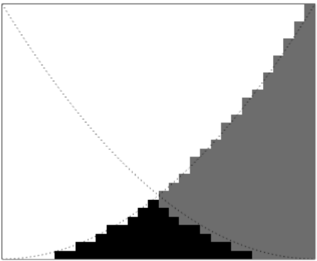As an example, consider P ( y < (1 -x ) 2 | x, y ∈ [0 , 1) ∧ y < x 2 ) . We can consider this to be the limiting value of P ( A n | X n ) as n →∞ , where the queries A n and premises X n are defined as follows: 1. Symbols a i and b i , for 1 ≤ i ≤ n , are intended to mean i -1 ≤ nx < i and i -1 ≤ ny < i respectively. 2. Let A n be ∨ ( i,j ) ∈ K ( a i ∧ b j ) where K = { ( i, j ): j/n ≤ (1 -i/n ) 2 } . 3. Let X n be ∨ ( i,j ) ∈ L ( a i ∧ b j ) where L = { ( i, j ): j/n ≤ ( i/n ) 2 } . Figure 9.1 illustrates X n ∧ A n in black and X n ∧ ¬ A n in gray for n = 30 . As n →∞ , A n tends in the limit to the desired query ' y < (1 -x ) 2 ' and X n tends in the limit to the desired premise ' y < x 2 ,' with x, y ∈ [0 , 1) implicit in the problem encoding. Though straightforward, it would be tedious to have to explicitly construct the limiting process and find the limiting value every time we considered a probability involving an infinite domain. Modern probability theory is based on measure theory, so it should be no surprise that measure theory provides the tools to automate this process of constructing a sequence of finite approximations that converge to a limit. We will not attempt to provide a full account of this large topic. By way of illustration, however, we will discuss one particularly simple case. We only sketch things out here; see Appendix Appendix A for more details. Consider the Cantor set of infinite binary sequences B ω , where B = { 0 , 1 } . Enumerating the elements of S as s 1 , s 2 , . . . , we can consider B ω to be the set of truth assignments on S if we identify a truth assignment ρ with the infinite sequence w such that w i = ρ ( s i ) for all i . We write C and µ C for the Borel Figure 9.1: Approximating P ( y < (1 -x ) 2 | y < x 2 ) with n = 30 <details> <summary>Image 1 Details</summary>  ### Visual Description ## Diagram: Staircase Approximation of a Curve ### Overview The image shows a square diagram with a curve approximated by two sets of staircases. One staircase is black and located near the bottom, while the other is gray and located near the top-right corner. A dotted line represents the curve being approximated. ### Components/Axes * **Axes:** The diagram is a square, implying equal scales on both axes, though no explicit labels are provided. The axes range from 0 to 1 implicitly. * **Curve:** A dotted line represents the curve being approximated. It starts at the top-left corner and curves downwards to the bottom-right corner. * **Black Staircase:** A black staircase pattern approximates the curve from below, near the bottom of the square. * **Gray Staircase:** A gray staircase pattern approximates the curve from above, near the top-right corner of the square. ### Detailed Analysis * **Curve Approximation:** The staircases provide a visual representation of approximating the area under the curve. The black staircase represents an underestimation, while the gray staircase represents an overestimation. * **Staircase Steps:** The steps of the staircases are uniform in size. * **Positioning:** The black staircase is positioned at the bottom of the square, while the gray staircase is positioned at the top-right corner. ### Key Observations * The dotted line is a curve that starts at the top-left corner and ends at the bottom-right corner. * The black staircase is below the curve, and the gray staircase is above the curve. * The staircases provide a visual representation of approximating the area under the curve. ### Interpretation The diagram illustrates the concept of approximating the area under a curve using step functions (staircases). The black staircase represents a lower bound (underestimation), while the gray staircase represents an upper bound (overestimation) of the true area under the curve. This is a visual representation of the concept of integration using Riemann sums. The dotted line represents the function being integrated. The diagram demonstrates how finer steps in the staircase would lead to a more accurate approximation of the area under the curve. </details> σ -algebra on B ω and Borel measure on C respectively, which may be considered a uniform distribution over B ω . Defining $$[ A ] = \{ w \in \mathbb { B } ^ { \omega } \colon w s a t i s f i e s \, A \}$$ $${ P r } \left ( { \tilde { A } } ; { \tilde { X } } , \mu \right ) = { \frac { \mu \left ( { \tilde { A } } \cap { \tilde { X } } \right ) } { \mu \left ( { \tilde { X } } \right ) } }$$ for any two measurable sets ˜ A, ˜ X and measure µ with µ ( ˜ X ) > 0 , we find that $$P \left ( A | X \right ) = P r \left ( [ A ] ; [ X ] , \mu _ { c } \right ) .$$ Finally, Theorem 26 (Appendix Appendix A) states that for any measurable sets ˜ A, ˜ X ∈ C with µ C ( ˜ X ) > 0 there exists a sequence of formulas A i ∈ Φ( S ) and X i ∈ Φ + ( S ) such that $$\mu _ { \mathcal { C } } \left ( [ A _ { i } ] \bigtriangleup \tilde { A } \right ) & \to 0 \\ \mu _ { \mathcal { C } } \left ( [ X _ { i } ] \bigtriangleup \tilde { X } \right ) & \to 0 \\ P \left ( A _ { i } \ | \ X _ { i } \right ) & \to \Pr \left ( \tilde { A } ; \tilde { X } , \mu _ { \mathcal { C } } \right )$$ $$1$$ as i → ∞ , where stands for set difference. That is, Jaynes's 'well-defined and well-behaved limiting process' is guaranteed to exist under the conditions of the Theorem, and Pr ( ˜ A ; ˜ X,µ C ) is the limiting probability. Now we turn to the space Ω = B m × [0 , 1) n . We write D for the powerset of B m (the maximal σ -algebra on B m ) and define µ D ( ˜ A ) = ∣ ∣ ∣ ˜ A ∣ ∣ ∣ / 2 m for ˜ A ∈ D . for any A ∈ Φ( S ) , and We write B and µ B for the Borel σ -algebra on [0 , 1) n and Borel measure on B , respectively. Let A = σ ( D×B ) be the product σ -algebra of D and B , and let µ A = µ D × µ B be the product measure of µ D and µ B . The measure µ A may be considered a uniform distribution over B m × [0 , 1) n , with µ A ( ˜ A × ˜ B ) being ∣ ∣ ∣ ˜ A ∣ ∣ ∣ / 2 m times the n -dimensional hypervolume of ˜ B . The set B ∗ 1 ω of binary sequences ending in an infinite sequence of 1's is a measurable set of measure 0. Let us define I = B ω \ B ∗ 1 ω to be all infinite binary sequences except this measure-0 set. Define the function f : I → Ω as <!-- formula-not-decoded --> That is, applying the mapping f amounts to interpreting symbol s m + ι ( i,j ) , for i ≥ 1 and 1 ≤ j ≤ n , as the i -th bit in the infinite binary expansion of x j ∈ [0 , 1) , or more precisely, as the proposition ' ⌊ 2 i x j ⌋ mod 2 = 1 .' We interleave n infinite sequences into one sequence by mapping index i of sequence j to index ι ( i, j ) of the combined sequence. Using symbols s m +1 through s m + ι ( k,n ) we can express any subspace of [0 , 1) n at a granularity of hypercubes of length 2 -k on each side, and we can make this granularity as fine as desired by choosing k sufficiently large. The function f is a bijection between I and Ω . (We excluded B ∗ 1 ω to ensure this, as dyadic rationals m/ 2 n have two possible binary expansions.) Furthermore, both f and f -1 are measurable: f -1 ( A ) ∈ C and f -1 ( A ) ⊆ I whenever A ⊆ A , and f ( B ) ∈ A whenever B ∈ C and B ⊆ I . Finally, f is measurepreserving: µ C ( f -1 ( A ) ) = µ A ( A ) whenever A ∈ A . This guarantees that $$\Pr \left ( \tilde { A } ; \tilde { X } , \mu _ { A } \right ) = P r \left ( f ^ { - 1 } \left ( \tilde { A } \right ) ; f ^ { - 1 } \left ( \tilde { X } \right ) , \mu _ { C } \right ) .$$ Therefore, we can apply Theorem 26 and find that for any measurable sets ˜ A, ˜ X ∈ A with µ A ( ˜ X ) > 0 there exist sequences of formulas A i and X i , with X i satisfiable, such that $$\mu _ { \mathcal { C } } \left ( [ A _ { i } ] \, \triangle f ^ { - 1 } \left ( \tilde { A } \right ) \right ) & \to 0 \\ \mu _ { \mathcal { C } } \left ( [ X _ { i } ] \, \triangle f ^ { - 1 } \left ( \tilde { X } \right ) \right ) & \to 0$$ as i →∞ . In the example given at the beginning of this section, we have m = 0 , n = 2 , and $$\begin{array} { r l } & { \tilde { A } = \left \{ ( x , y ) \in [ 0 , 1 ) ^ { 2 } \colon y < ( 1 - x ) ^ { 2 } \right \} } \\ & { \tilde { X } = \left \{ ( x , y ) \in [ 0 , 1 ) ^ { 2 } \colon y < x ^ { 2 } \right \} . } \end{array}$$ $$1$$ The above results tell us that we don't need to explicitly construct the sequence of approximating formulas for this example; it is guaranteed to exist, and the limiting probability is $${ P r } \left ( \tilde { A } ; \tilde { X } , \mu _ { \mathcal { A } } \right ) = \frac { \int _ { 0 } ^ { 1 } \min \left ( x ^ { 2 } , \left ( 1 - x \right ) ^ { 2 } \right ) d x } { \int _ { 0 } ^ { 1 } x ^ { 2 } d x } = \frac { 1 } { 4 } .$$ As another example, let us revisit and generalize the inductive model described in Section 9.2: $$\theta \sim D i s t r \left ( F \right ) \\ x _ { i } \sim B e r n o u l l i ( \theta ) \quad i n d e p e n d e n t l y f o r a l l 1 \leq i \leq I$$ where Distr( F ) is the distribution on the unit interval with cdf F , which we take to be continuous (and hence invertible). Doing a change of variables and augmenting with latent variables s i , the above is equivalent to $$p \sim \text {Uniform} ( 0 , 1 ) \\ \theta = F ^ { - 1 } ( p ) \\ s _ { i } \sim \text {Uniform} ( 0 , 1 ) x _ { i } & = \begin{cases} 1 & \text {if $s_{i}<\theta$} \\ 0 & \text {otherwise} \end{cases} \\ \text {W.} & \text {theorem} \quad \text {and} \quad \text {otherwise}$$ after marginalizing out p and s . We have independent uniform distributions on p and each s i , plus equations relating each x i to p and s i ; hence the above is equivalent to using as premise the measurable set $$\tilde { X } = \left \{ ( x , p , s ) \in \mathbb { B } ^ { I } \times [ 0 , 1 ) ^ { 1 + I } \colon x _ { i } = 1 \Leftrightarrow s _ { i } < F ^ { - 1 } \left ( p \right ) \, f o r a l l \ 1 \leq i \leq I \right \} ,$$ again using the σ -algebra A and measure µ A , with m = I and n = I +1 . For any measurable ˜ A we are again guaranteed that Pr ( ˜ A ; ˜ X,µ A ) is the limiting probability obtained from a sequence of approximating formulas A i and X i . This is not a complete solution to handling infinite problem domains. For instance, in the example above we used B I (with finite I ) instead of B ω , because µ A ( ˜ X ) → 0 as I → ∞ . In addition, the measure µ C on C and encoding of real numbers used above works well for a bounded interval like [0 , 1) but does not suffice for unbounded intervals, such as all of R . For such cases we need alternative measures on C and corresponding analogs to Theorem 26, along with alternative encodings for these domains. Other work that remains to be done on this topic includes the following: 1. Finding a general method of constructing the needed sequence of approximating formulas for any computable probability measure [10, 22]. 2. Extending our language of propositional formulas to express measurable sets beyond just the cylinder sets, while ensuring that P ( A | X ) remains computable, as is appropriate for a logical system. We have made some initial investigations of these open issues and believe that they can be resolved. ## 10. Conclusion We have strengthened the case for probability theory as the uniquely determined extension of classical propositional logic to a logic of plausible reasoning. Our proof relies on a small and simple set of requirements such a logic must satisfy. These requirements are harder to dispute than those of previous such efforts because every one of the requirements is motivated by a desire to retain in our extended logic some property of CPL. A crucial distinction between our approach and similar previous work is that A | X depends only on the explicit arguments A and X , and not on any other domain-specific or problem-specific information; any such relevant information must be included in the premise X . This makes the plausibility function a legitimate analog of the logical consequence relation: the truth or falsity of X | = A likewise depends only on X and A , and not on any implicit domain-specific or problem-specific information. R2 (invariance under definition of new symbols) in conjunction with R1 (logical equivalence) turns out to have far-reaching implications. It yields invariance under renaming of propositional symbols and, in fact, a fully general invariance under change-of-variable transformations. Most importantly, it implies that A | X is a function only of # S ( A ∧ X ) and # S ( X ) for any S containing all the symbols used in A and X . R3 (invariance under addition of irrelevant information) excludes Carnap's system, which comes pre-supplied with dependencies between propositions rather than letting any dependencies be specified in the premise. Adding R3 implies that A | X is a function of the ratio of # S ( A ∧ X ) to # S ( X ) . Finally, with R4 we made use of the underappreciated fact that CPL already comes equipped with an inherent plausibility ordering on propositions, for any given premise. The invariances of R1-R3 'stitch together' these partial orderings for distinct premises, and we find that we have an order-preserving isomorphism P between the set of plausibilities P and the set of rational probabilities Q 01 . The numeric value we find for P ( A | X ) recreates the classical definition of probability, but in a sharper, clearer form with the troublesome circularity excised, and as a theorem rather than as a definition. The 'possible cases' are identified as truth assignments satisfying the premise, and the meaning of 'equally possible cases' is simply that we have no additional information that would expand the satisfying truth assignments by differing multiplicities. We addressed two possible concerns about our result: that it seems to allow only uniform probabilities, and that it yields probabilities only for finite domains. We showed how non-uniform probabilities arise via the introduction of latent variables, along with information in the premise linking these latent variables to the observables. Following Jaynes, we proposed that probabilities for infinite domains be obtained via a well-defined and well-behaved limiting process, and demonstrated how measure theory can automate the construction of such limiting processes in at least some cases. ## Appendix A. Measure Theory Appendix A.1. Some results from measure theory We assume the reader is already familiar with the basic concepts of measure theory: an algebra, a σ -algebra, a measurable set, the σ -algebra σ ( A ) generated by an algebra A , a measurable function, a measure on an algebra or σ -algebra, and a σ -finite measure. Billingsley [3] and Tao [19] are good references. Here we highlight some results we will use. A measure on an algebra A can always be consistently extended to a measure on σ ( A ) [3, Theorem 11.3]: Theorem 17. If µ is a measure on an algebra A then µ extends to a measure on σ ( A ) , that is, there exists a measure µ ′ on σ ( A ) such that µ ( A ) = µ ′ ( A ) for all A ∈ A . If µ is σ -finite then µ ′ is unique, and is also σ -finite. In many cases of interest the elements of a σ -algebra can be approximated arbitrarily closely by sets from the generating algebra [3, Theorem 11.4]: Theorem 18. If A is an algebra on Ω , µ is a σ -finite measure on σ ( A ) , and B ∈ σ ( A ) with µ ( B ) < ∞ , then for every > 0 there exists some A ∈ A such that µ ( A B ) < . We use the following measure-related properties of set differences A B , which we state without proof: Property 19. For any measure µ on an algebra A and any A,B ∈ A , $$\left | \mu ( A ) - \mu ( B ) \right | \leq \mu \left ( A \triangle B \right ) .$$ Property 20. For any measure µ on an algebra A and any A 1 , A 2 , X 1 , X 2 ∈ A , $$\mu \left ( \left ( A _ { 1 } \cap X _ { 1 } \right ) \triangle \left ( A _ { 2 } \cap X _ { 2 } \right ) \right ) \leq \mu \left ( A _ { 1 } \triangle A _ { 2 } \right ) + \mu \left ( X _ { 1 } \triangle X _ { 2 } \right ) .$$ Appendix A.2. Constructing the 'well-defined and well-behaved limiting process' To avoid confusion between propositional formulas and measurable sets, in this section we will generally decorate the names of measurable sets with a tilde ( ˜ A , ˜ B , etc.) and leave the names of propositional formulas undecorated ( A , B , etc.) The Borel σ -algebra and Borel measure for the Cantor set B ω are constructed as follows: Definition 21. A cylinder set is a subset of B ω of the form cyl ( n, C ) C B ω for some C ⊆ B n . C 0 is the collection of all cylinder sets. This set is an algebra, and the Borel σ -algebra for B ω is C σ ( C 0 ) , the σ -algebra generated by C 0 . Cylinder sets are the basis of a topology on B ω in which the open sets are any finite or countable union of cylinder sets, and this is why we call C the Borel σ -agebra for B ω . Definition 22. The Borel measure for C is the measure µ C such that $$\mu _ { \mathcal { C } } \left ( c y l \left ( n , C \right ) \right ) = 2 ^ { - n } \left | C \right |$$ for any n ≥ 0 and C ⊆ B n . The definition above is unambiguous because cyl( n, C ) = cyl( n + m,C ′ ) if and only if C ′ = C B m . Note that µ C is trivially σ -finite, since B ω itself is a cylinder set and µ C ( B ω ) is finite. By Theorem 17 µ C is uniquely defined once we define its value on cylinder sets. Let us enumerate the elements of S as s 1 , s 2 , . . . and identify a sequence w ∈ B ω with the truth assignment ρ on S such that ρ ( s i ) = w i for all i ; then every propositional formula corresponds to a cylinder set: Definition 23. If A is a propositional formula then [ A ] is the set of w ∈ B ω that satisfy A (considered as truth assignments.) Note that [ A ] = cyl( n, C ) and µ C ([ A ]) = 2 -n # S ( A ) , where σ J A K ⊆ S = { s 1 , . . . , s n } and C is the set of w ∈ B n that satisfy A . Likewise, every cylinder set corresponds to a propositional formula: Lemma 24. For any cylinder set ˜ A there is a formula A ∈ Φ( S ) such that ˜ A = [ A ] . Proof. Let ˜ A = cyl ( n, C ) and define the propositional formula A as $$A & = \bigvee _ { c \in C } A _ { c } \\ A _ { c } & = \bigwedge _ { i = 1 } ^ { n } L _ { i , c _ { i } }$$ It is straightforward to see that [ A ] = ˜ A . We can define an analog to P ( A | X ) , but for measurable sets: Definition 25. Let A be a σ -algebra and µ a measure on A . For any ˜ A, ˜ X ∈ A with µ ( ˜ X ) > 0 , define $${ P r } \left ( { \tilde { A } ; \tilde { X } , \mu } \right ) = { \frac { \mu \left ( { \tilde { A } \cap \tilde { X } } \right ) } { \mu \left ( { \tilde { X } } \right ) } } .$$ We then find that $$P \left ( A | X \right ) = { \frac { 2 ^ { - n } \# _ { S } \left ( A \wedge X \right ) } { 2 ^ { - n } \# _ { S } \left ( X \right ) } } = P r \left ( [ A ] ; [ X ] , \mu _ { C } \right )$$ where we choose n to be large enough that σ J A,X K ⊆ S = { s 1 , . . . , s n } . We use this fact to show that Jaynes's 'well-defined and well-behaved limiting process' is guaranteed to exist for measurable sets: Theorem 26. Let ˜ A, ˜ X ∈ C , with µ C ( ˜ X ) > 0 . Then there exists a sequence of formulas A i ∈ Φ( S ) and X i ∈ Φ + ( S ) such that $$1 . \, \lim _ { i \to \infty } \mu _ { \mathcal { C } } \left ( [ A _ { i } ] \bigtriangleup \tilde { A } \right ) = 0 .$$ $$\begin{array} { r } { 2 . \, l i m _ { i \rightarrow \infty } \mu _ { \mathcal { C } } \left ( [ X _ { i } ] \triangle \tilde { X } \right ) = 0 . } \end{array}$$ $$\begin{array} { r } { 3 . \, l i m _ { i \rightarrow \infty } P \left ( A _ { i } | X _ { i } \right ) = P r \left ( \tilde { A } ; \tilde { X } , \mu _ { c } \right ) . } \end{array}$$ Proof. Let i , i ≥ 1 be any decreasing sequence of positive numbers whose limit is 0, with 1 < µ C ( ˜ X ) . Using Theorem 18 and Lemma 24 we can define $$A _ { i } & = \text {some} \ A \in \Phi \left ( \mathcal { S } \right ) \text { such that } \mu _ { \mathcal { C } } \left ( [ A ] \triangle \tilde { A } \right ) < \epsilon _ { i } \\ X _ { i } & = \text {some} \ X \in \Phi \left ( \mathcal { S } \right ) \text { such that } \mu _ { \mathcal { C } } \left ( [ X ] \triangle \tilde { X } \right ) < \epsilon _ { i }$$ 1 and 2 in the theorem statement follow directly from these definitions. From Property 19 we have $$\left | \mu _ { \mathcal { C } } \left ( [ X _ { i } ] \right ) - \mu _ { \mathcal { C } } \left ( \tilde { X } \right ) \right | \leq \mu _ { \mathcal { C } } \left ( [ X ] \triangle \tilde { X } \right ) < \epsilon _ { i } < \mu _ { \mathcal { C } } \left ( \tilde { X } \right )$$ and so µ C ([ X i ]) > 0 , i.e., X i is satisfiable. Property 19 also gives us $$\lim _ { i \rightarrow \infty } \mu _ { \mathcal { C } } \left ( [ X _ { i } ] \right ) = \mu _ { \mathcal { C } } \left ( \tilde { X } \right ) .$$ $$\mu _ { \mathcal { C } } \left ( [ A _ { i } \wedge X _ { i } ] \bigtriangleup \left ( \tilde { A } \cap \tilde { X } \right ) \right ) < 2 \epsilon _ { i }$$ and then Property 19 yields $$\lim _ { i \to \infty } \mu _ { \mathcal { C } } \left ( [ A _ { i } \wedge X _ { i } ] \right ) = \mu _ { \mathcal { C } } \left ( \tilde { A } \cap \tilde { X } \right ) .$$ Property 20 gives us Finally we have $$\lim _ { i \rightarrow \infty } P \left ( A _ { i } \, | \, X _ { i } \right ) = \lim _ { i \rightarrow \infty } \frac { \mu _ { \mathcal { C } } \left ( [ A _ { i } \wedge X _ { i } ] \right ) } { \mu _ { \mathcal { C } } \left ( [ X _ { i } ] \right ) } = \frac { \mu _ { \mathcal { C } } \left ( \tilde { A } \cap \tilde { X } \right ) } { \mu _ { \mathcal { C } } \left ( \tilde { X } \right ) } = P r \left ( \tilde { A } ; \tilde { X } , \mu _ { \mathcal { C } } \right ) .$$ ## References - [1] Aczél, J. (1996). Lectures on Functional Equations and Their Applications . Academic Press. - [2] Bertrand, J. (1889). Calcul des Probabilites . Gauthier-Villars. - [3] Billingsley, P. (1995). Probability and Measure, Third Edition . John Wiley & Sons. - [4] Cardano, G. (1564). Liber de Ludo Aleae. - [5] Carnap, R. (1962). Logical Foundations of Probability (2nd edition). University of Chicago Press. - [6] Carnap, R. (1952). The Continuum of Inductive Methods . University of Chicago Press. - [7] Clayton, A., and T. Waddington (2017). 'Bridging the intuition gap in Cox's Theorem: A Jaynesian argument for universality.' International Journal of Approximate Reasoning 80 , 36-51. - [8] Colyvan, M. (2004). 'The philosophical significance of Cox's theorem.' International Journal of Approximate Reasoning 37 (1), 71-85. - [9] Cox, R. T., 1946. 'Probability, frequency and reasonable expectation.' American Journal of Physics 14 (1), 1-13. - [10] Edalat, A. (2009). 'A computable approach to measure and integration theory.' Information and Computation 207 , 642-659. - [11] Halpern, J. Y. (1999) 'A Counterexample to Theorems of Cox and Fine.' Journal of Artificial Intelligence Research 10 , pp. 67-85. - [12] Halpern, J. Y., (1999), 'Technical addendum: Cox's Theorem revisited.' Journal of Artificial Intelligence Research 11 , 429-435. - [13] Jaynes, E. T. (2003). Probability Theory: The Logic of Science . Cambridge University Press. - [14] Johnstone, P. T. (1987). Notes on Logic and Set Theory (1st edition). Cambridge University Press. - [15] Laplace, P.-S. (1812). Théorie Analytique des Probabilités , Volume 2. - [16] Paris, J. B. (1994). The Uncertain Reasoner's Companion: A Mathematical Perspective . Cambridge University Press. - [17] Pólya, G. (1954). Mathematics and Plausible Reasoning: Vol 2: Patterns of Plausible Inference. Oxford University Press. - [18] Shafer, G. (2004). 'Comments on constructing a logic of plausible inference: a guide to Cox's Theorem, by Kevin S. Van Horn.' International Journal of Approximate Reasoning 35 (1), 97-105. - [19] Tao, T. (2011). An Introduction to Measure Theory . American Mathematical Society. - [20] Tribus, M. (1969). Rational Descriptions, Decisions, and Designs . Pergamon Press. - [21] Van Horn, K. S. (2003). 'Constructing a logic of plausible inference: a guide to Cox's Theorem.' International Journal of Approximate Reasoning 34 (1), 3-24. - [22] Weihrauch, K. and N. R. Tavana (2014). 'Representations of measurable sets in computable measure theory.' Logical Methods in Computer Science 10 (3:7), 1-21.