## A Tutorial on Thompson Sampling
Daniel J. Russo 1 , Benjamin Van Roy 2 , Abbas Kazerouni 2 , Ian Osband 3 and Zheng Wen 4
1 Columbia University
2 Stanford University
3 Google DeepMind
4 Adobe Research
## ABSTRACT
Thompson sampling is an algorithm for online decision problems where actions are taken sequentially in a manner that must balance between exploiting what is known to maximize immediate performance and investing to accumulate new information that may improve future performance. The algorithm addresses a broad range of problems in a computationally efficient manner and is therefore enjoying wide use. This tutorial covers the algorithm and its application, illustrating concepts through a range of examples, including Bernoulli bandit problems, shortest path problems, product recommendation, assortment, active learning with neural networks, and reinforcement learning in Markov decision processes. Most of these problems involve complex information structures, where information revealed by taking an action informs beliefs about other actions. We will also discuss when and why Thompson sampling is or is not effective and relations to alternative algorithms.
In memory of Arthur F. Veinott, Jr.
## 1 Introduction
The multi-armed bandit problem has been the subject of decades of intense study in statistics, operations research, electrical engineering, computer science, and economics. A 'one-armed bandit' is a somewhat antiquated term for a slot machine, which tends to 'rob' players of their money. The colorful name for our problem comes from a motivating story in which a gambler enters a casino and sits down at a slot machine with multiple levers, or arms, that can be pulled. When pulled, an arm produces a random payout drawn independently of the past. Because the distribution of payouts corresponding to each arm is not listed, the player can learn it only by experimenting. As the gambler learns about the arms' payouts, she faces a dilemma: in the immediate future she expects to earn more by exploiting arms that yielded high payouts in the past, but by continuing to explore alternative arms she may learn how to earn higher payouts in the future. Can she develop a sequential strategy for pulling arms that balances this tradeoff and maximizes the cumulative payout earned? The following Bernoulli bandit problem is a canonical example.
Example 1.1. ( Bernoulli Bandit ) Suppose there are K actions, and when played, any action yields either a success or a failure. Action
k ∈ { 1 , ..., K } produces a success with probability θ k ∈ [0 , 1]. The success probabilities ( θ 1 , .., θ K ) are unknown to the agent, but are fixed over time, and therefore can be learned by experimentation. The objective, roughly speaking, is to maximize the cumulative number of successes over T periods, where T is relatively large compared to the number of arms K .
The 'arms' in this problem might represent different banner ads that can be displayed on a website. Users arriving at the site are shown versions of the website with different banner ads. A success is associated either with a click on the ad, or with a conversion (a sale of the item being advertised). The parameters θ k represent either the click-throughrate or conversion-rate among the population of users who frequent the site. The website hopes to balance exploration and exploitation in order to maximize the total number of successes.
A naive approach to this problem involves allocating some fixed fraction of time periods to exploration and in each such period sampling an arm uniformly at random, while aiming to select successful actions in other time periods. We will observe that such an approach can be quite wasteful even for the simple Bernoulli bandit problem described above and can fail completely for more complicated problems.
Problems like the Bernoulli bandit described above have been studied in the decision sciences since the second world war, as they crystallize the fundamental trade-off between exploration and exploitation in sequential decision making. But the information revolution has created significant new opportunities and challenges, which have spurred a particularly intense interest in this problem in recent years. To understand this, let us contrast the Internet advertising example given above with the problem of choosing a banner ad to display on a highway. A physical banner ad might be changed only once every few months, and once posted will be seen by every individual who drives on the road. There is value to experimentation, but data is limited, and the cost of of trying a potentially ineffective ad is enormous. Online, a different banner ad can be shown to each individual out of a large pool of users, and data from each such interaction is stored. Small-scale experiments are now a core tool at most leading Internet companies.
Our interest in this problem is motivated by this broad phenomenon. Machine learning is increasingly used to make rapid data-driven decisions. While standard algorithms in supervised machine learning learn passively from historical data, these systems often drive the generation of their own training data through interacting with users. An online recommendation system, for example, uses historical data to optimize current recommendations, but the outcomes of these recommendations are then fed back into the system and used to improve future recommendations. As a result, there is enormous potential benefit in the design of algorithms that not only learn from past data, but also explore systemically to generate useful data that improves future performance. There are significant challenges in extending algorithms designed to address Example 1.1 to treat more realistic and complicated decision problems. To understand some of these challenges, consider the problem of learning by experimentation to solve a shortest path problem.
Example 1.2. (Online Shortest Path) An agent commutes from home to work every morning. She would like to commute along the path that requires the least average travel time, but she is uncertain of the travel time along different routes. How can she learn efficiently and minimize the total travel time over a large number of trips?
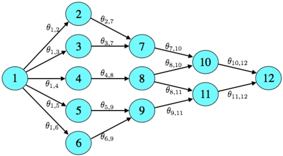
Figure 1.1: Shortest path problem.
<details>
<summary>Image 1 Details</summary>
### Visual Description
## Diagram: Directed Acyclic Graph
### Overview
The image depicts a directed acyclic graph (DAG) with 12 nodes, numbered 1 through 12. The nodes are represented as light blue circles, and the directed edges are represented as black arrows. Each edge is labeled with a theta value, denoted as θ followed by the source and destination node numbers. The graph starts with node 1, which branches out to nodes 2, 3, 4, 5, and 6. These nodes then connect to nodes 7, 8, 9, 10, 11, and finally converge at node 12.
### Components/Axes
* **Nodes:** 1, 2, 3, 4, 5, 6, 7, 8, 9, 10, 11, 12 (represented as light blue circles)
* **Edges:** Directed arrows connecting the nodes. Each edge is labeled with a theta value.
* **Edge Labels:** θ<sub>source, destination</sub> (e.g., θ<sub>1,2</sub>, θ<sub>2,7</sub>)
### Detailed Analysis or Content Details
* **Node 1** has outgoing edges to nodes 2, 3, 4, 5, and 6. The corresponding edge labels are θ<sub>1,2</sub>, θ<sub>1,3</sub>, θ<sub>1,4</sub>, θ<sub>1,5</sub>, and θ<sub>1,6</sub>.
* **Node 2** has an outgoing edge to node 7, labeled θ<sub>2,7</sub>.
* **Node 3** has an outgoing edge to node 7, labeled θ<sub>3,7</sub>.
* **Node 4** has an outgoing edge to node 8, labeled θ<sub>4,8</sub>.
* **Node 5** has an outgoing edge to node 9, labeled θ<sub>5,9</sub>.
* **Node 6** has an outgoing edge to node 9, labeled θ<sub>6,9</sub>.
* **Node 7** has an outgoing edge to node 10, labeled θ<sub>7,10</sub>.
* **Node 8** has outgoing edges to nodes 10 and 11, labeled θ<sub>8,10</sub> and θ<sub>8,11</sub>.
* **Node 9** has an outgoing edge to node 11, labeled θ<sub>9,11</sub>.
* **Node 10** has an outgoing edge to node 12, labeled θ<sub>10,12</sub>.
* **Node 11** has an outgoing edge to node 12, labeled θ<sub>11,12</sub>.
* **Node 12** has no outgoing edges.
### Key Observations
* The graph starts with a single node (1) and ends with a single node (12).
* The graph branches out from node 1 and converges at node 12.
* Nodes 7, 8, 9, 10, and 11 have multiple incoming edges.
* The graph is acyclic, meaning there are no cycles or loops.
### Interpretation
The diagram represents a directed acyclic graph, which is a common structure used in various fields such as computer science, project management, and decision-making. The nodes can represent tasks, events, or states, and the edges represent dependencies or relationships between them. The theta values associated with the edges could represent weights, probabilities, or costs associated with traversing those edges. The graph illustrates a process that starts with a single initial state (node 1), branches into multiple parallel paths, and eventually converges to a final state (node 12). The specific meaning of the graph depends on the context in which it is used.
</details>
We can formalize this as a shortest path problem on a graph G = ( V, E ) with vertices V = { 1 , ..., N } and edges E . An example is illustrated in Figure 1.1. Vertex 1 is the source (home) and vertex N is the destination (work). Each vertex can be thought of as an intersection, and for two vertices i, j ∈ V , an edge ( i, j ) ∈ E is present if there is a direct road connecting the two intersections. Suppose that traveling along an edge e ∈ E requires time θ e on average. If these parameters were known, the agent would select a path ( e 1 , .., e n ), consisting of a sequence of adjacent edges connecting vertices 1 and N , such that the expected total time θ e 1 + ... + θ e n is minimized. Instead, she chooses paths in a sequence of periods. In period t , the realized time y t,e to traverse edge e is drawn independently from a distribution with mean θ e . The agent sequentially chooses a path x t , observes the realized travel time ( y t,e ) e ∈ x t along each edge in the path, and incurs cost c t = ∑ e ∈ x t y t,e equal to the total travel time. By exploring intelligently, she hopes to minimize cumulative travel time ∑ T t =1 c t over a large number of periods T .
This problem is conceptually similar to the Bernoulli bandit in Example 1.1, but here the number of actions is the number of paths in the graph, which generally scales exponentially in the number of edges. This raises substantial challenges. For moderate sized graphs, trying each possible path would require a prohibitive number of samples, and algorithms that require enumerating and searching through the set of all paths to reach a decision will be computationally intractable. An efficient approach therefore needs to leverage the statistical and computational structure of problem.
In this model, the agent observes the travel time along each edge traversed in a given period. Other feedback models are also natural: the agent might start a timer as she leaves home and checks it once she arrives, effectively only tracking the total travel time of the chosen path. This is closer to the Bernoulli bandit model, where only the realized reward (or cost) of the chosen arm was observed. We have also taken the random edge-delays y t,e to be independent, conditioned on θ e . A more realistic model might treat these as correlated random variables, reflecting that neighboring roads are likely to be congested at the same time. Rather than design a specialized algorithm for each possible statistical
model, we seek a general approach to exploration that accommodates flexible modeling and works for a broad array of problems. We will see that Thompson sampling accommodates such flexible modeling, and offers an elegant and efficient approach to exploration in a wide range of structured decision problems, including the shortest path problem described here.
Thompson sampling - also known as posterior sampling and probability matching - was first proposed in 1933 (Thompson, 1933; Thompson, 1935) for allocating experimental effort in two-armed bandit problems arising in clinical trials. The algorithm was largely ignored in the academic literature until recently, although it was independently rediscovered several times in the interim (Wyatt, 1997; Strens, 2000) as an effective heuristic. Now, more than eight decades after it was introduced, Thompson sampling has seen a surge of interest among industry practitioners and academics. This was spurred partly by two influential articles that displayed the algorithm's strong empirical performance (Chapelle and Li, 2011; Scott, 2010). In the subsequent five years, the literature on Thompson sampling has grown rapidly. Adaptations of Thompson sampling have now been successfully applied in a wide variety of domains, including revenue management (Ferreira et al. , 2015), marketing (Schwartz et al. , 2017), web site optimization (Hill et al. , 2017), Monte Carlo tree search (Bai et al. , 2013), A/B testing (Graepel et al. , 2010), Internet advertising (Graepel et al. , 2010; Agarwal, 2013; Agarwal et al. , 2014), recommendation systems (Kawale et al. , 2015), hyperparameter tuning (Kandasamy et al. , 2018), and arcade games (Osband et al. , 2016a); and have been used at several companies, including Adobe, Amazon (Hill et al. , 2017), Facebook, Google (Scott, 2010; Scott, 2015), LinkedIn (Agarwal, 2013; Agarwal et al. , 2014), Microsoft (Graepel et al. , 2010), Netflix, and Twitter.
The objective of this tutorial is to explain when, why, and how to apply Thompson sampling. A range of examples are used to demonstrate how the algorithm can be used to solve a variety of problems and provide clear insight into why it works and when it offers substantial benefit over naive alternatives. The tutorial also provides guidance on approximations to Thompson sampling that can simplify computation
as well as practical considerations like prior distribution specification, safety constraints and nonstationarity. Accompanying this tutorial we also release a Python package 1 that reproduces all experiments and figures presented. This resource is valuable not only for reproducible research, but also as a reference implementation that may help practioners build intuition for how to practically implement some of the ideas and algorithms we discuss in this tutorial. A concluding section discusses theoretical results that aim to develop an understanding of why Thompson sampling works, highlights settings where Thompson sampling performs poorly, and discusses alternative approaches studied in recent literature. As a baseline and backdrop for our discussion of Thompson sampling, we begin with an alternative approach that does not actively explore.
1 Python code and documentation is available at https://github.com/iosband/ ts\_tutorial.
## Greedy Decisions
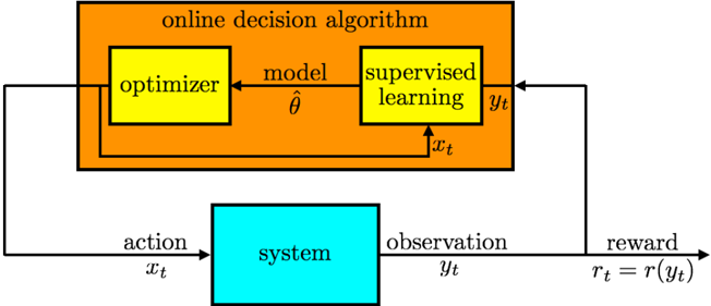
Greedy algorithms serve as perhaps the simplest and most common approach to online decision problems. The following two steps are taken to generate each action: (1) estimate a model from historical data and (2) select the action that is optimal for the estimated model, breaking ties in an arbitrary manner. Such an algorithm is greedy in the sense that an action is chosen solely to maximize immediate reward. Figure 2.1 illustrates such a scheme. At each time t , a supervised learning algorithm fits a model to historical data pairs H t -1 = (( x 1 , y 1 ) , . . . , ( x t -1 , y t -1 )), generating an estimate ˆ θ of model parameters. The resulting model can then be used to predict the reward r t = r ( y t ) from applying action x t . Here, y t is an observed outcome, while r is a known function that represents the agent's preferences. Given estimated model parameters ˆ θ , an optimization algorithm selects the action x t that maximizes expected reward, assuming that θ = ˆ θ . This action is then applied to the exogenous system and an outcome y t is observed.
A shortcoming of the greedy approach, which can severely curtail performance, is that it does not actively explore. To understand this issue, it is helpful to focus on the Bernoulli bandit setting of Example 1.1. In that context, the observations are rewards, so r t = r ( y t ) = y t .
Figure 2.1: Online decision algorithm.
<details>
<summary>Image 2 Details</summary>
### Visual Description
## Diagram: Online Decision Algorithm
### Overview
The image is a block diagram illustrating an online decision algorithm interacting with a system. The algorithm consists of an optimizer and a supervised learning component, which exchange information to make decisions that affect the system. The system, in turn, provides observations back to the algorithm, closing the loop.
### Components/Axes
* **Title:** "online decision algorithm" (located at the top, within the orange box)
* **Components:**
* "optimizer" (yellow box, top-left within the orange box)
* "supervised learning" (yellow box, top-right within the orange box)
* "system" (cyan box, bottom center)
* **Variables:**
* "model" (above the arrow from optimizer to supervised learning), represented by the symbol "θ" (theta) with a hat.
* "action" (above the arrow from the online decision algorithm to the system), represented by "x_t".
* "observation" (above the arrow from the system to the online decision algorithm), represented by "y_t".
* "reward" (above the arrow from the system back to the online decision algorithm), represented by "r_t = r(y_t)".
### Detailed Analysis
The diagram shows the flow of information and actions between the online decision algorithm and the system.
1. **Online Decision Algorithm:** The algorithm, enclosed in an orange box, contains two main components:
* **Optimizer:** The optimizer (yellow box) generates a "model" (θ with a hat) that is sent to the supervised learning component.
* **Supervised Learning:** The supervised learning component (yellow box) receives the model and the action "x_t" from the system. It outputs "y_t".
2. **System:** The system (cyan box) receives an "action" (x_t) from the online decision algorithm. Based on this action, the system produces an "observation" (y_t) and a "reward" (r_t = r(y_t)).
3. **Feedback Loop:** The "observation" (y_t) is fed back to the supervised learning component, and the "reward" (r_t) is fed back to the optimizer, closing the feedback loop.
### Key Observations
* The diagram illustrates a closed-loop control system where the online decision algorithm learns and adapts based on the system's response to its actions.
* The optimizer and supervised learning components work together to make decisions.
* The reward signal is a function of the observation, indicating that the algorithm's performance is evaluated based on the system's state.
### Interpretation
The diagram represents a reinforcement learning or adaptive control system. The online decision algorithm learns to control the system by observing its behavior and adjusting its actions to maximize the reward. The optimizer likely updates the model based on the reward signal, while the supervised learning component uses the model and observations to predict the system's future state or to select the best action. The feedback loop allows the algorithm to continuously improve its performance over time. The diagram highlights the key components and interactions involved in this type of system.
</details>
At each time t , a greedy algorithm would generate an estimate ˆ θ k of the mean reward for each k th action, and select the action that attains the maximum among these estimates.
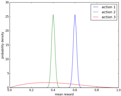
Suppose there are three actions with mean rewards θ ∈ R 3 . In particular, each time an action k is selected, a reward of 1 is generated with probability θ k . Otherwise, a reward of 0 is generated. The mean rewards are not known to the agent. Instead, the agent's beliefs in any given time period about these mean rewards can be expressed in terms of posterior distributions. Suppose that, conditioned on the observed history H t -1 , posterior distributions are represented by the probability density functions plotted in Figure 2.2. These distributions represent beliefs after the agent tries actions 1 and 2 one thousand times each, action 3 three times, receives cumulative rewards of 600, 400, and 1, respectively, and synthesizes these observations with uniform prior distributions over mean rewards of each action. They indicate that the agent is confident that mean rewards for actions 1 and 2 are close to their expectations of approximately 0 . 6 and 0 . 4. On the other hand, the agent is highly uncertain about the mean reward of action 3, though he expects 0 . 4.
The greedy algorithm would select action 1, since that offers the maximal expected mean reward. Since the uncertainty around this expected mean reward is small, observations are unlikely to change the expectation substantially, and therefore, action 1 is likely to be selected
Figure 2.2: Probability density functions over mean rewards.
<details>
<summary>Image 3 Details</summary>
### Visual Description
## Chart: Probability Density vs. Mean Reward for Different Actions
### Overview
The image is a chart displaying probability density functions for three different actions, plotted against the mean reward. Each action is represented by a different colored line, showing the distribution of potential rewards associated with that action.
### Components/Axes
* **X-axis:** "mean reward", ranging from 0.0 to 1.0 in increments of 0.2.
* **Y-axis:** "probability density", ranging from 0 to 30.
* **Legend (top-right):**
* Blue line: "action 1"
* Green line: "action 2"
* Red line: "action 3"
### Detailed Analysis
* **Action 1 (Blue):** The probability density function for action 1 is a narrow peak centered around a mean reward of approximately 0.6. The peak probability density is approximately 26.
* **Action 2 (Green):** The probability density function for action 2 is a narrow peak centered around a mean reward of approximately 0.4. The peak probability density is approximately 25.
* **Action 3 (Red):** The probability density function for action 3 is a wide, shallow curve. The peak probability density is approximately 1.5, occurring around a mean reward of approximately 0.2.
### Key Observations
* Actions 1 and 2 have much higher peak probability densities than action 3, indicating more certainty in their respective mean rewards.
* Action 1 has the highest mean reward (approximately 0.6), followed by action 2 (approximately 0.4), and then action 3 (approximately 0.2).
* Action 3 has a much wider distribution, indicating a higher degree of uncertainty in the potential rewards.
### Interpretation
The chart suggests that action 1 is the most likely to yield a high reward, as it has both a high mean reward and a high probability density. Action 2 is also likely to yield a reward, but with a slightly lower mean. Action 3, while still potentially yielding a reward, has a much lower probability density and a lower mean reward, making it a less desirable choice. The narrow peaks of actions 1 and 2 indicate that the rewards are more predictable, while the wide distribution of action 3 suggests a higher degree of risk or variability.
</details>
ad infinitum . It seems reasonable to avoid action 2, since it is extremely unlikely that θ 2 > θ 1 . On the other hand, if the agent plans to operate over many time periods, it should try action 3. This is because there is some chance that θ 3 > θ 1 , and if this turns out to be the case, the agent will benefit from learning that and applying action 3. To learn whether θ 3 > θ 1 , the agent needs to try action 3, but the greedy algorithm will unlikely ever do that. The algorithm fails to account for uncertainty in the mean reward of action 3, which should entice the agent to explore and learn about that action.
Dithering is a common approach to exploration that operates through randomly perturbing actions that would be selected by a greedy algorithm. One version of dithering, called /epsilon1 -greedy exploration , applies the greedy action with probability 1 -/epsilon1 and otherwise selects an action uniformly at random. Though this form of exploration can improve behavior relative to a purely greedy approach, it wastes resources by failing to 'write off' actions regardless of how unlikely they are to be optimal. To understand why, consider again the posterior distributions of Figure 2.2. Action 2 has almost no chance of being optimal, and therefore, does not deserve experimental trials, while the uncertainty surrounding action 3 warrants exploration. However, /epsilon1 -greedy explo-
ration would allocate an equal number of experimental trials to each action. Though only half of the exploratory actions are wasted in this example, the issue is exacerbated as the number of possible actions increases. Thompson sampling, introduced more than eight decades ago (Thompson, 1933), provides an alternative to dithering that more intelligently allocates exploration effort.
## Thompson Sampling for the Bernoulli Bandit
To digest how Thompson sampling (TS) works, it is helpful to begin with a simple context that builds on the Bernoulli bandit of Example 1.1 and incorporates a Bayesian model to represent uncertainty.
Example 3.1. (Beta-Bernoulli Bandit) Recall the Bernoulli bandit of Example 1.1. There are K actions. When played, an action k produces a reward of one with probability θ k and a reward of zero with probability 1 -θ k . Each θ k can be interpreted as an action's success probability or mean reward. The mean rewards θ = ( θ 1 , ..., θ K ) are unknown, but fixed over time. In the first period, an action x 1 is applied, and a reward r 1 ∈ { 0 , 1 } is generated with success probability P ( r 1 = 1 | x 1 , θ ) = θ x 1 . After observing r 1 , the agent applies another action x 2 , observes a reward r 2 , and this process continues.
Let the agent begin with an independent prior belief over each θ k . Take these priors to be beta-distributed with parameters α = ( α 1 , . . . , α K ) and β ∈ ( β 1 , . . . , β K ). In particular, for each action k , the prior probability density function of θ k is
$$p ( \theta _ { k } ) = \frac { \Gamma ( \alpha _ { k } + \beta _ { k } ) } { \Gamma ( \alpha _ { k } ) \Gamma ( \beta _ { k } ) } \theta _ { k } ^ { \alpha _ { k } - 1 } ( 1 - \theta _ { k } ) ^ { \beta _ { k } - 1 } ,$$
where Γ denotes the gamma function. As observations are gathered, the distribution is updated according to Bayes' rule. It is particularly convenient to work with beta distributions because of their conjugacy properties. In particular, each action's posterior distribution is also beta with parameters that can be updated according to a simple rule:
/negationslash
$$( \alpha _ { k } , \beta _ { k } ) \leftarrow \begin{cases} ( \alpha _ { k } , \beta _ { k } ) & i f x _ { t } \neq k \\ ( \alpha _ { k } , \beta _ { k } ) + ( r _ { t } , 1 - r _ { t } ) & i f x _ { t } = k . \end{cases}$$
Note that for the special case of α k = β k = 1, the prior p ( θ k ) is uniform over [0 , 1]. Note that only the parameters of a selected action are updated. The parameters ( α k , β k ) are sometimes called pseudocounts, since α k or β k increases by one with each observed success or failure, respectively. A beta distribution with parameters ( α k , β k ) has mean α k / ( α k + β k ), and the distribution becomes more concentrated as α k + β k grows. Figure 2.2 plots probability density functions of beta distributions with parameters ( α 1 , β 1 ) = (601 , 401), ( α 2 , β 2 ) = (401 , 601), and ( α 3 , β 3 ) = (2 , 3).
Algorithm 3.1 presents a greedy algorithm for the beta-Bernoulli bandit. In each time period t , the algorithm generates an estimate ˆ θ k = α k / ( α k + β k ), equal to its current expectation of the success probability θ k . The action x t with the largest estimate ˆ θ k is then applied, after which a reward r t is observed and the distribution parameters α x t and β x t are updated.
TS, specialized to the case of a beta-Bernoulli bandit, proceeds similarly, as presented in Algorithm 3.2. The only difference is that the success probability estimate ˆ θ k is randomly sampled from the posterior distribution, which is a beta distribution with parameters α k and β k , rather than taken to be the expectation α k / ( α k + β k ). To avoid a common misconception, it is worth emphasizing TS does not sample ˆ θ k from the posterior distribution of the binary value y t that would be observed if action k is selected. In particular, ˆ θ k represents a statistically plausible success probability rather than a statistically plausible observation.
Algorithm 3.1 BernGreedy( K,α,β ) 1: for t = 1 , 2 , . . . do 2: #estimate model: 3: for k = 1 , . . . , K do 4: ˆ θ k ← α k / ( α k + β k ) 5: end for 6: 7: #select and apply action: 8: x t ← argmax k ˆ θ k 9: Apply x t and observe r t 10: 11: #update distribution: 12: ( α x t , β x t ) ← ( α x t + r t , β x t +1 -r t ) 13: end for
## Algorithm 3.2 BernTS( K,α,β )
```
Algorithm 3.2 BernTS(K, \alpha, \beta)
1: for t = 1, 2,... do
2: #sample model:
3: for k = 1, ..., K do
4: Sample $\hat{k}_k^{\theta_k} \quad$ end for
5: end for
7: #select and apply action:
8: x_t <- argmax_{\hat{k}_k}
9: Apply x_t and observe $r_t$
10:
11: end for
```
To understand how TS improves on greedy actions with or without dithering, recall the three armed Bernoulli bandit with posterior distributions illustrated in Figure 2.2. In this context, a greedy action would forgo the potentially valuable opportunity to learn about action 3. With dithering, equal chances would be assigned to probing actions 2 and 3, though probing action 2 is virtually futile since it is extremely unlikely to be optimal. TS, on the other hand would sample actions 1, 2, or 3, with probabilities approximately equal to 0 . 82, 0, and 0 . 18, respectively. In each case, this is the probability that the random estimate drawn for the action exceeds those drawn for other actions. Since these estimates are drawn from posterior distributions, each of these probabilities is also equal to the probability that the corresponding action is optimal, conditioned on observed history. As such, TS explores to resolve uncertainty where there is a chance that resolution will help the agent identify the optimal action, but avoids probing where feedback would not be helpful.
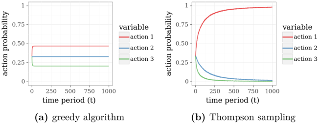
It is illuminating to compare simulated behavior of TS to that of a greedy algorithm. Consider a three-armed beta-Bernoulli bandit with mean rewards θ 1 = 0 . 9, θ 2 = 0 . 8, and θ 3 = 0 . 7. Let the prior distribution over each mean reward be uniform. Figure 3.1 plots results based on ten thousand independent simulations of each algorithm. Each simulation is over one thousand time periods. In each simulation, actions
are randomly rank-ordered for the purpose of tie-breaking so that the greedy algorithm is not biased toward selecting any particular action. Each data point represents the fraction of simulations for which a particular action is selected at a particular time.
Figure 3.1: Probability that the greedy algorithm and Thompson sampling selects an action.
<details>
<summary>Image 4 Details</summary>
### Visual Description
## Chart: Action Probability vs. Time Period for Greedy Algorithm and Thompson Sampling
### Overview
The image presents two line charts comparing the action probabilities over time for a greedy algorithm and Thompson sampling. Each chart displays three actions (action 1, action 2, and action 3) with their probabilities plotted against the time period.
### Components/Axes
* **Left Chart (a) - Greedy Algorithm:**
* X-axis: "time period (t)" ranging from 0 to 1000.
* Y-axis: "action probability" ranging from 0 to 1.
* Legend (top-right):
* Red: "action 1"
* Blue: "action 2"
* Green: "action 3"
* **Right Chart (b) - Thompson Sampling:**
* X-axis: "time period (t)" ranging from 0 to 1000.
* Y-axis: "action probability" ranging from 0 to 1.
* Legend (top-right):
* Red: "action 1"
* Blue: "action 2"
* Green: "action 3"
### Detailed Analysis
**Left Chart (a) - Greedy Algorithm:**
* **Action 1 (Red):** Starts at approximately 0.45 at time period 0, quickly rises to approximately 0.50, and remains relatively constant around 0.50 for the rest of the time period.
* **Action 2 (Blue):** Starts at approximately 0.35 at time period 0 and remains relatively constant around 0.35 for the rest of the time period.
* **Action 3 (Green):** Starts at approximately 0.20 at time period 0 and remains relatively constant around 0.20 for the rest of the time period.
**Right Chart (b) - Thompson Sampling:**
* **Action 1 (Red):** Starts at approximately 0.45 at time period 0, rapidly increases to approximately 0.98, and remains relatively constant around 0.98 for the rest of the time period.
* **Action 2 (Blue):** Starts at approximately 0.35 at time period 0, rapidly decreases to approximately 0.02, and remains relatively constant around 0.02 for the rest of the time period.
* **Action 3 (Green):** Starts at approximately 0.20 at time period 0, rapidly decreases to approximately 0.01, and remains relatively constant around 0.01 for the rest of the time period.
### Key Observations
* In the greedy algorithm, the action probabilities remain relatively stable over time.
* In Thompson sampling, action 1 quickly dominates, while actions 2 and 3 diminish rapidly.
### Interpretation
The charts illustrate the difference in behavior between a greedy algorithm and Thompson sampling in a multi-armed bandit problem. The greedy algorithm explores all actions with relatively stable probabilities, while Thompson sampling quickly converges to a single action (action 1) and exploits it, suppressing the probabilities of the other actions. This demonstrates Thompson sampling's ability to quickly identify and exploit the most rewarding action, while the greedy algorithm maintains a more balanced exploration strategy.
</details>
From the plots, we see that the greedy algorithm does not always converge on action 1, which is the optimal action. This is because the algorithm can get stuck, repeatedly applying a poor action. For example, suppose the algorithm applies action 3 over the first couple time periods and receives a reward of 1 on both occasions. The algorithm would then continue to select action 3, since the expected mean reward of either alternative remains at 0 . 5. With repeated selection of action 3, the expected mean reward converges to the true value of 0 . 7, which reinforces the agent's commitment to action 3. TS, on the other hand, learns to select action 1 within the thousand periods. This is evident from the fact that, in an overwhelmingly large fraction of simulations, TS selects action 1 in the final period.
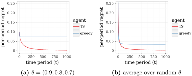
The performance of online decision algorithms is often studied and compared through plots of regret. The per-period regret of an algorithm over a time period t is the difference between the mean reward of an optimal action and the action selected by the algorithm. For the Bernoulli bandit problem, we can write this as regret t ( θ ) = max k θ k -θ x t . Figure 3.2a plots per-period regret realized by the greedy algorithm and TS, again averaged over ten thousand simulations. The average
per-period regret of TS vanishes as time progresses. That is not the case for the greedy algorithm.
Comparing algorithms with fixed mean rewards raises questions about the extent to which the results depend on the particular choice of θ . As such, it is often useful to also examine regret averaged over plausible values of θ . A natural approach to this involves sampling many instances of θ from the prior distributions and generating an independent simulation for each. Figure 3.2b plots averages over ten thousand such simulations, with each action reward sampled independently from a uniform prior for each simulation. Qualitative features of these plots are similar to those we inferred from Figure 3.2a, though regret in Figure 3.2a is generally smaller over early time periods and larger over later time periods, relative to Figure 3.2b. The smaller regret in early time periods is due to the fact that with θ = (0 . 9 , 0 . 8 , 0 . 7), mean rewards are closer than for a typical randomly sampled θ , and therefore the regret of randomly selected actions is smaller. The fact that per-period regret of TS is larger in Figure 3.2a than Figure 3.2b over later time periods, like period 1000, is also a consequence of proximity among rewards with θ = (0 . 9 , 0 . 8 , 0 . 7). In this case, the difference is due to the fact that it takes longer to differentiate actions than it would for a typical randomly sampled θ .
Figure 3.2: Regret from applying greedy and Thompson sampling algorithms to the three-armed Bernoulli bandit.
<details>
<summary>Image 5 Details</summary>
### Visual Description
## Line Graphs: Per-Period Regret vs. Time Period for Different Agents
### Overview
The image presents two line graphs comparing the per-period regret of two agents, "TS" (Thompson Sampling) and "greedy," over time. The x-axis represents the time period (t), ranging from 0 to 1000. The y-axis represents the per-period regret, ranging from 0 to 0.25. The left graph (a) shows results for a specific parameter set θ = (0.9, 0.8, 0.7), while the right graph (b) shows results averaged over random θ.
### Components/Axes
* **X-axis (Horizontal):** "time period (t)". Scale ranges from 0 to 1000, with tick marks at 0, 250, 500, 750, and 1000.
* **Y-axis (Vertical):** "per-period regret". Scale ranges from 0 to 0.25, with tick marks at 0, 0.05, 0.10, 0.15, 0.20, and 0.25.
* **Legend (Top-Right of each graph):**
* "TS" - Red line
* "greedy" - Blue line
* **Graph Titles:**
* (a) θ = (0.9, 0.8, 0.7)
* (b) average over random θ
### Detailed Analysis
**Graph (a): θ = (0.9, 0.8, 0.7)**
* **TS (Red Line):** The per-period regret starts at approximately 0.075 at time period 0 and rapidly decreases, approaching 0 as the time period increases. By time period 1000, the regret is close to 0.
* **Greedy (Blue Line):** The per-period regret remains relatively constant at approximately 0.075 across all time periods.
**Graph (b): Average over random θ**
* **TS (Red Line):** The per-period regret starts at approximately 0.225 at time period 0 and decreases rapidly, approaching 0 as the time period increases. By time period 1000, the regret is close to 0.
* **Greedy (Blue Line):** The per-period regret starts at approximately 0.08 at time period 0 and decreases slightly, stabilizing at approximately 0.035 as the time period increases.
### Key Observations
* In both graphs, the "TS" agent exhibits a decreasing per-period regret over time, indicating learning and improved performance.
* In graph (a), the "greedy" agent maintains a constant regret, suggesting no learning.
* In graph (b), the "greedy" agent shows a slight decrease in regret, but not as significant as the "TS" agent.
* The initial regret for the "TS" agent is much higher in graph (b) compared to graph (a), but it still converges to a low regret value.
### Interpretation
The graphs demonstrate that the Thompson Sampling (TS) agent consistently outperforms the greedy agent in terms of minimizing per-period regret over time. The TS agent's ability to learn and adapt to the environment results in a significant reduction in regret, while the greedy agent either maintains a constant regret or shows only a slight improvement. The difference in initial regret for the TS agent between the two graphs suggests that the performance of the TS agent is sensitive to the specific parameter set θ. However, even when averaged over random θ, the TS agent still converges to a low regret value, indicating its robustness and effectiveness.
</details>
## General Thompson Sampling
TS can be applied fruitfully to a broad array of online decision problems beyond the Bernoulli bandit, and we now consider a more general setting. Suppose the agent applies a sequence of actions x 1 , x 2 , x 3 , . . . to a system, selecting each from a set X . This action set could be finite, as in the case of the Bernoulli bandit, or infinite. After applying action x t , the agent observes an outcome y t , which the system randomly generates according to a conditional probability measure q θ ( ·| x t ). The agent enjoys a reward r t = r ( y t ), where r is a known function. The agent is initially uncertain about the value of θ and represents his uncertainty using a prior distribution p .
Algorithms 4.1 and 4.2 present greedy and TS approaches in an abstract form that accommodates this very general problem. The two differ in the way they generate model parameters ˆ θ . The greedy algorithm takes ˆ θ to be the expectation of θ with respect to the distribution p , while TS draws a random sample from p . Both algorithms then apply actions that maximize expected reward for their respective models. Note that, if there are a finite set of possible observations y t , this expectation is given by
$$\mathbb { E } _ { q _ { \hat { \theta } } } [ r ( y _ { t } ) | x _ { t } = x ] = \sum _ { o } q _ { \hat { \theta } } ( o | x ) r ( o ) .$$
The distribution p is updated by conditioning on the realized observation ˆ y t . If θ is restricted to values from a finite set, this conditional distribution can be written by Bayes rule as
$$( 4 . 2 ) \quad \mathbb { P } _ { p , q } ( \theta = u | x _ { t } , y _ { t } ) = \frac { p ( u ) q _ { u } ( y _ { t } | x _ { t } ) } { \sum _ { v } p ( v ) q _ { v } ( y _ { t } | x _ { t } ) } .$$
## Algorithm 4.1 Greedy( X , p, q, r )
```
Algorithm 4.1 Greedy(X,p,q,r)
1: for t = 1,2,... do
2: #estimate model:
3: $\theta \leftarrow \mathbb{E}_{p}[\theta]$
4:
5: $#select and apply action:
6: x_{t \leftarrow argmax_{x\in\mathcal{X}\,q_0^{\theta}}[r(y_{t})|x_{t = x}]$
7:
8: Apply x_{t and observe y_{t}$
9:
10: #update distribution:
11: p \leftarrow \mathbb{P}_{p,q}(\theta \in \cdot | x_{t},y_{t})$
12: end for
```
## Algorithm
4.2
Thompson( X , p, q, r )
```
\frac{1: for t = 1,2,... do
2: #sample model:
3: Sample $\hat{\theta} \sim p
4: #select and apply action:
5: x_{t <- argmax_{x\in\mathbb{E}q_\hat{y}(r(y_t)|x_t = x)}
6: Apply $x_t$ and observe $y_t
7: }
8: #update distribution:
9: p <- \mathbb{P}_{p,q}(\theta \in \cdot|x_{t}, y_{t})
```
The Bernoulli bandit with a beta prior serves as a special case of this more general formulation. In this special case, the set of actions is X = { 1 , . . . , K } and only rewards are observed, so y t = r t . Observations and rewards are modeled by conditional probabilities q θ (1 | k ) = θ k and q θ (0 | k ) = 1 -θ k . The prior distribution is encoded by vectors α and β , with probability density function given by:
$$p ( \theta ) = \prod _ { k = 1 } ^ { K } \frac { \Gamma ( \alpha + \beta ) } { \Gamma ( \alpha _ { k } ) \Gamma ( \beta _ { k } ) } \theta _ { k } ^ { \alpha _ { k } - 1 } ( 1 - \theta _ { k } ) ^ { \beta _ { k } - 1 } ,$$
where Γ denotes the gamma function. In other words, under the prior distribution, components of θ are independent and beta-distributed, with parameters α and β .
For this problem, the greedy algorithm (Algorithm 4.1) and TS (Algorithm 4.2) begin each t th iteration with posterior parameters ( α k , β k ) for k ∈ { 1 , . . . , K } . The greedy algorithm sets ˆ θ k to the expected value E p [ θ k ] = α k / ( α k + β k ), whereas TS randomly draws ˆ θ k from a beta distribution with parameters ( α k , β k ). Each algorithm then selects the action x that maximizes E q ˆ θ [ r ( y t ) | x t = x ] = ˆ θ x . After applying the
selected action, a reward r t = y t is observed, and belief distribution parameters are updated according to
$$( \alpha , \beta ) \gets ( \alpha + r _ { t } 1 _ { x _ { t } } , \beta + ( 1 - r _ { t } ) 1 _ { x _ { t } } ) ,$$
where 1 x t is a vector with component x t equal to 1 and all other components equal to 0.
Algorithms 4.1 and 4.2 can also be applied to much more complex problems. As an example, let us consider a version of the shortest path problem presented in Example 1.2.
Example 4.1. (Independent Travel Times) Recall the shortest path problem of Example 1.2. The model is defined with respect to a directed graph G = ( V, E ), with vertices V = { 1 , . . . , N } , edges E , and mean travel times θ ∈ R N . Vertex 1 is the source and vertex N is the destination. An action is a sequence of distinct edges leading from source to destination. After applying action x t , for each traversed edge e ∈ x t , the agent observes a travel time y t,e that is independently sampled from a distribution with mean θ e . Further, the agent incurs a cost of ∑ e ∈ x t y t,e , which can be thought of as a reward r t = -∑ e ∈ x t y t,e .
Consider a prior for which each θ e is independent and log-Gaussiandistributed with parameters µ e and σ 2 e . That is, ln( θ e ) ∼ N ( µ e , σ 2 e ) is Gaussian-distributed. Hence, E [ θ e ] = e µ e + σ 2 e / 2 . Further, take y t,e | θ to be independent across edges e ∈ E and log-Gaussian-distributed with parameters ln( θ e ) -˜ σ 2 / 2 and ˜ σ 2 , so that E [ y t,e | θ e ] = θ e . Conjugacy properties accommodate a simple rule for updating the distribution of θ e upon observation of y t,e :
$$( 4 . 3 ) \quad ( \mu _ { e } , \sigma _ { e } ^ { 2 } ) \leftarrow \left ( \frac { \frac { 1 } { \sigma _ { e } ^ { 2 } } \mu _ { e } + \frac { 1 } { \tilde { \sigma } ^ { 2 } } \left ( \ln ( y _ { t , e } ) + \frac { \tilde { \sigma } ^ { 2 } } { 2 } \right ) } { \frac { 1 } { \sigma _ { e } ^ { 2 } } + \frac { 1 } { \tilde { \sigma } ^ { 2 } } } , \frac { 1 } { \frac { 1 } { \sigma _ { e } ^ { 2 } } + \frac { 1 } { \tilde { \sigma } ^ { 2 } } } \right ) .$$
To motivate this formulation, consider an agent who commutes from home to work every morning. Suppose possible paths are represented by a graph G = ( V, E ). Suppose the agent knows the travel distance d e associated with each edge e ∈ E but is uncertain about average travel times. It would be natural for her to construct a prior for which expectations are equal to travel distances. With the log-Gaussian prior, this can be accomplished by setting µ e = ln( d e ) -σ 2 e / 2. Note that the
parameters µ e and σ 2 e also express a degree of uncertainty; in particular, the prior variance of mean travel time along an edge is ( e σ 2 e -1) d 2 e .
The greedy algorithm (Algorithm 4.1) and TS (Algorithm 4.2) can be applied to Example 4.1 in a computationally efficient manner. Each algorithm begins each t th iteration with posterior parameters ( µ e , σ e ) for each e ∈ E . The greedy algorithm sets ˆ θ e to the expected value E p [ θ e ] = e µ e + σ 2 e / 2 , whereas TS randomly draws ˆ θ e from a log-Gaussian distribution with parameters µ e and σ 2 e . Each algorithm then selects its action x to maximize E q ˆ θ [ r ( y t ) | x t = x ] = -∑ e ∈ x t ˆ θ e . This can be cast as a deterministic shortest path problem, which can be solved efficiently, for example, via Dijkstra's algorithm. After applying the selected action, an outcome y t is observed, and belief distribution parameters ( µ e , σ 2 e ), for each e ∈ E , are updated according to (4.3).
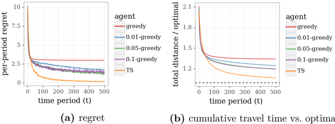
Figure 4.1 presents results from applying greedy and TS algorithms to Example 4.1, with the graph taking the form of a binomial bridge, as shown in Figure 4.2, except with twenty rather than six stages, so there are 184,756 paths from source to destination. Prior parameters are set to µ e = -1 2 and σ 2 e = 1 so that E [ θ e ] = 1, for each e ∈ E , and the conditional distribution parameter is ˜ σ 2 = 1. Each data point represents an average over ten thousand independent simulations.
The plots of regret demonstrate that the performance of TS converges quickly to optimal, while that is far from true for the greedy algorithm. We also plot results generated by /epsilon1 -greedy exploration, varying /epsilon1 . For each trip, with probability 1 -/epsilon1 , this algorithm traverses a path produced by a greedy algorithm. Otherwise, the algorithm samples a path randomly. Though this form of exploration can be helpful, the plots demonstrate that learning progresses at a far slower pace than with TS. This is because /epsilon1 -greedy exploration is not judicious in how it selects paths to explore. TS, on the other hand, orients exploration effort towards informative rather than entirely random paths.
Plots of cumulative travel time relative to optimal offer a sense for the fraction of driving time wasted due to lack of information. Each point plots an average of the ratio between the time incurred over some number of days and the minimal expected travel time given θ . With TS, this converges to one at a respectable rate. The same can not be said for /epsilon1 -greedy approaches.
Figure 4.1: Performance of Thompson sampling and /epsilon1 -greedy algorithms in the shortest path problem.
<details>
<summary>Image 6 Details</summary>
### Visual Description
## Chart Type: Comparative Line Graphs
### Overview
The image presents two line graphs comparing the performance of different agents in a decision-making task. Graph (a) shows the "per-period regret" over time, while graph (b) displays the "cumulative travel time vs. optimal" over time. Five different agents are compared: "greedy", "0.01-greedy", "0.05-greedy", "0.1-greedy", and "TS" (likely Thompson Sampling).
### Components/Axes
**Graph (a): Regret**
* **Title:** per-period regret
* **X-axis:** time period (t), ranging from 0 to 500
* **Y-axis:** per-period regret, ranging from 0 to 10
* **Agents (Legend, top-right of graph (a)):**
* Red: greedy
* Blue: 0.01-greedy
* Green: 0.05-greedy
* Purple: 0.1-greedy
* Orange: TS
**Graph (b): Cumulative Travel Time vs. Optimal**
* **Title:** total distance / optimal
* **X-axis:** time period (t), ranging from 0 to 500
* **Y-axis:** total distance / optimal, ranging from 1.2 to 2.1
* **Agents (Legend, top-right of graph (b)):**
* Red: greedy
* Blue: 0.01-greedy
* Green: 0.05-greedy
* Purple: 0.1-greedy
* Orange: TS
* A horizontal dashed grey line is present at y=1.0
### Detailed Analysis
**Graph (a): Regret**
* **Greedy (Red):** Starts at approximately 3 and remains relatively constant around 3.
* **0.01-greedy (Blue):** Starts around 5, decreases rapidly initially, then plateaus around 1.5 after t=200.
* **0.05-greedy (Green):** Starts around 7, decreases rapidly initially, then plateaus around 1.5 after t=200.
* **0.1-greedy (Purple):** Starts around 7, decreases rapidly initially, then plateaus around 1.5 after t=200.
* **TS (Orange):** Starts around 10, decreases rapidly, and plateaus near 0 after t=200.
**Graph (b): Cumulative Travel Time vs. Optimal**
* **Greedy (Red):** Starts at approximately 1.35 and remains relatively constant around 1.35.
* **0.01-greedy (Blue):** Starts around 1.6, decreases rapidly initially, then plateaus around 1.3 after t=200.
* **0.05-greedy (Green):** Starts around 1.8, decreases rapidly initially, then plateaus around 1.3 after t=200.
* **0.1-greedy (Purple):** Starts around 1.9, decreases rapidly initially, then plateaus around 1.25 after t=200.
* **TS (Orange):** Starts around 2.1, decreases rapidly, and approaches 1.1 after t=200.
### Key Observations
* The "TS" agent consistently outperforms the other agents in both metrics, achieving the lowest regret and cumulative travel time relative to the optimal.
* The "greedy" agent performs the worst, showing the highest regret and cumulative travel time.
* The epsilon-greedy agents (0.01, 0.05, 0.1) show similar performance, with higher epsilon values leading to slightly lower cumulative travel time.
* All agents except the greedy agent show a significant decrease in regret and cumulative travel time during the initial time periods, eventually plateauing.
### Interpretation
The graphs demonstrate the trade-offs between exploration and exploitation in decision-making. The "greedy" agent, which only exploits the current best option, performs poorly. The epsilon-greedy agents explore with a small probability, leading to better performance. The "TS" agent, which uses Thompson Sampling to balance exploration and exploitation, achieves the best performance. The data suggests that a well-balanced exploration strategy is crucial for minimizing regret and achieving near-optimal performance in this task. The fact that the TS agent's cumulative travel time approaches 1.1 suggests it is performing close to the theoretical optimum.
</details>
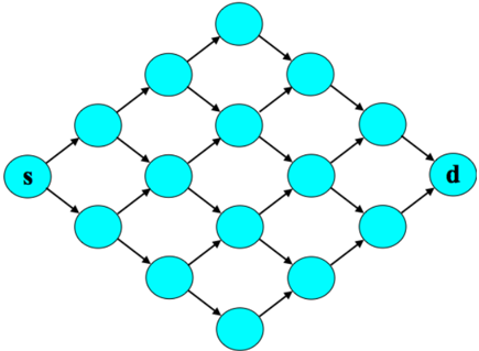
Figure 4.2: A binomial bridge with six stages.
<details>
<summary>Image 7 Details</summary>
### Visual Description
## Diagram: Directed Acyclic Graph
### Overview
The image depicts a directed acyclic graph (DAG) with nodes arranged in a diamond shape. The graph starts with a node labeled "s" and ends with a node labeled "d". The nodes are connected by directed edges, indicating the flow from "s" to "d".
### Components/Axes
* **Nodes:** The graph consists of 16 nodes, each represented by a cyan-filled circle. Two nodes are labeled "s" (start) and "d" (destination).
* **Edges:** The nodes are connected by black arrows, indicating the direction of the graph.
* **Labels:** The start node is labeled "s" and the destination node is labeled "d".
### Detailed Analysis
The graph can be visualized as a grid of nodes arranged in a diamond shape. The start node "s" is located on the left side of the diamond, and the destination node "d" is located on the right side. The arrows indicate the possible paths from "s" to "d".
The graph has the following structure:
* **Level 1:** 1 node (s)
* **Level 2:** 2 nodes
* **Level 3:** 3 nodes
* **Level 4:** 4 nodes
* **Level 5:** 3 nodes
* **Level 6:** 2 nodes
* **Level 7:** 1 node (d)
Each node (except the nodes in the last level) has two outgoing edges, pointing to the nodes in the next level. Each node (except the nodes in the first level) has two incoming edges, coming from the nodes in the previous level.
### Key Observations
* The graph is directed and acyclic.
* The graph has a clear start and destination node.
* The graph has a diamond shape.
* The graph has multiple paths from "s" to "d".
### Interpretation
The diagram represents a directed acyclic graph, which is a type of graph where the edges have a direction and there are no cycles. This type of graph is often used to model processes or relationships where the order of events is important. In this case, the graph could represent a network, a workflow, or a decision tree. The multiple paths from "s" to "d" suggest that there are multiple ways to reach the destination. The diamond shape of the graph could be related to the complexity of the process, with the middle levels representing the most complex stages.
</details>
Algorithm 4.2 can be applied to problems with complex information structures, and there is often substantial value to careful modeling of such structures. As an example, we consider a more complex variation of the binomial bridge example.
Example 4.2. (Correlated Travel Times) As with Example 4.1, let each θ e be independent and log-Gaussian-distributed with parameters µ e and σ 2 e . Let the observation distribution be characterized by
$$y _ { t , e } = \zeta _ { t , e } \eta _ { t } \nu _ { t , \ell ( e ) } \theta _ { e } ,$$
where each ζ t,e represents an idiosyncratic factor associated with edge e , η t represents a factor that is common to all edges, /lscript ( e ) indicates whether edge e resides in the lower half of the binomial bridge, and ν t, 0 and ν t, 1 represent factors that bear a common influence on edges in the upper and lower halves, respectively. We take each ζ t,e , η t , ν t, 0 , and ν t, 1 to be independent log-Gaussian-distributed with parameters -˜ σ 2 / 6 and ˜ σ 2 / 3. The distributions of the shocks ζ t,e , η t , ν t, 0 and ν t, 1 are known, and only the parameters θ e corresponding to each individual edge must be learned through experimentation. Note that, given these parameters, the marginal distribution of y t,e | θ is identical to that of Example 4.1, though the joint distribution over y t | θ differs.
The common factors induce correlations among travel times in the binomial bridge: η t models the impact of random events that influence traffic conditions everywhere, like the day's weather, while ν t, 0 and ν t, 1 each reflect events that bear influence only on traffic conditions along edges in half of the binomial bridge. Though mean edge travel times are independent under the prior, correlated observations induce dependencies in posterior distributions.
Conjugacy properties again facilitate efficient updating of posterior parameters. Let φ, z t ∈ R N be defined by
$$\phi _ { e } = \ln ( \theta _ { e } ) \quad a n d \quad z _ { t , e } = \left \{ \begin{array} { l l } { \ln ( y _ { t , e } ) } & { i f e \in x _ { t } } \\ { 0 } & { o t h e r w i s e . } \end{array}$$
Note that it is with some abuse of notation that we index vectors and matrices using edge indices. Define a | x t | × | x t | covariance matrix ˜ Σ with elements
/negationslash
$$\tilde { \Sigma } _ { e , e ^ { \prime } } = \left \{ \begin{array} { l l } { \tilde { \sigma } ^ { 2 } } & { f o r e = e ^ { \prime } } \\ { 2 \tilde { \sigma } ^ { 2 } / 3 } & { f o r e \neq e ^ { \prime } , \ell ( e ) = \ell ( e ^ { \prime } ) } \\ { \tilde { \sigma } ^ { 2 } / 3 } & { o t h e r w i s e , } \end{array}$$
for e, e ′ ∈ x t , and a N × N concentration matrix
$$\tilde { C } _ { e , e ^ { \prime } } = \left \{ \begin{array} { l l } { \tilde { \Sigma } _ { e , e ^ { \prime } } ^ { - 1 } } & { i f e , e ^ { \prime } \in x _ { t } } \\ { 0 } & { o t h e r w i s e , } \end{array}$$
for e, e ′ ∈ E . Then, the posterior distribution of φ is Gaussian with a mean vector µ and covariance matrix Σ that can be updated according
to
$$\begin{array} { r l } { ( 4 . 4 ) } & \left ( \mu , \Sigma \right ) \leftarrow \left ( \left ( \Sigma ^ { - 1 } + \tilde { C } \right ) ^ { - 1 } \left ( \Sigma ^ { - 1 } \mu + \tilde { C } z _ { t } \right ) , \left ( \Sigma ^ { - 1 } + \tilde { C } \right ) ^ { - 1 } \right ) . } \end{array}$$
TS (Algorithm 4.2) can again be applied in a computationally efficient manner. Each t th iteration begins with posterior parameters µ ∈ R N and Σ ∈ R N × N . The sample ˆ θ can be drawn by first sampling a vector ˆ φ from a Gaussian distribution with mean µ and covariance matrix Σ, and then setting ˆ θ e = ˆ φ e for each e ∈ E . An action x is selected to maximize E q ˆ θ [ r ( y t ) | x t = x ] = -∑ e ∈ x t ˆ θ e , using Djikstra's algorithm or an alternative. After applying the selected action, an outcome y t is observed, and belief distribution parameters ( µ, Σ) are updated according to (4.4).
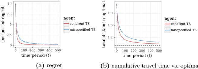
Figure 4.3: Performance of two versions of Thompson sampling in the shortest path problem with correlated travel times.
<details>
<summary>Image 8 Details</summary>
### Visual Description
## Chart: Agent Performance Comparison
### Overview
The image presents two line charts comparing the performance of two agents, "coherent TS" and "misspecified TS," over time. The left chart (a) shows the per-period regret, while the right chart (b) shows the cumulative travel time vs. optimal. Both charts display the performance of the two agents over 500 time periods.
### Components/Axes
**Left Chart (a): Regret**
* **Title:** per-period regret
* **X-axis:** time period (t), with markers at 0, 100, 200, 300, 400, and 500.
* **Y-axis:** per-period regret, with markers at 0, 2.5, 5, 7.5, and 10.
* **Legend (Top-Right):**
* Red line: coherent TS
* Blue line: misspecified TS
**Right Chart (b): Cumulative Travel Time vs. Optimal**
* **Title:** total distance / optimal
* **X-axis:** time period (t), with markers at 0, 100, 200, 300, 400, and 500.
* **Y-axis:** total distance / optimal, with markers at 1.2, 1.5, and 1.8.
* **Legend (Top-Right):**
* Red line: coherent TS
* Blue line: misspecified TS
* A dashed horizontal line is present at y=1.0.
### Detailed Analysis
**Left Chart (a): Regret**
* **Coherent TS (Red):** The regret starts at approximately 2.5 and decreases rapidly, approaching 0 after around 200 time periods.
* **Misspecified TS (Blue):** The regret starts at approximately 5 and decreases rapidly, approaching 0 after around 200 time periods.
**Right Chart (b): Cumulative Travel Time vs. Optimal**
* **Coherent TS (Red):** The total distance/optimal starts at approximately 1.5 and decreases, approaching 1.1 after 500 time periods.
* **Misspecified TS (Blue):** The total distance/optimal starts at approximately 1.9 and decreases, approaching 1.15 after 500 time periods.
### Key Observations
* Both agents show a decrease in per-period regret and total distance/optimal over time.
* The misspecified TS agent initially has a higher regret and total distance/optimal compared to the coherent TS agent.
* Both agents' performance converges over time, with their regret approaching 0 and their total distance/optimal approaching a similar value.
### Interpretation
The charts demonstrate the learning behavior of the two agents. Initially, the "misspecified TS" agent performs worse, indicating that its initial model or assumptions are not well-aligned with the environment. However, as both agents interact with the environment over time, they learn and adapt, leading to a reduction in regret and a decrease in the ratio of total distance to optimal distance. The convergence of performance suggests that both agents are eventually able to find near-optimal solutions, even if they start from different initial states or with different models. The dashed line at y=1.0 in the right chart represents the optimal travel time, and the agents are approaching this value as time progresses.
</details>
Figure 4.3 plots results from applying TS to Example 4.2, again with the binomial bridge, µ e = -1 2 , σ 2 e = 1, and ˜ σ 2 = 1. Each data point represents an average over ten thousand independent simulations. Despite model differences, an agent can pretend that observations made in this new context are generated by the model described in Example 4.1. In particular, the agent could maintain an independent log-Gaussian posterior for each θ e , updating parameters ( µ e , σ 2 e ) as though each y t,e | θ is independently drawn from a log-Gaussian distribution. As a baseline for comparison, Figure 4.3 additionally plots results from application of this approach, which we will refer to here as misspecified TS . The comparison demonstrates substantial improvement that results from
accounting for interdependencies among edge travel times, as is done by what we refer to here as coherent TS . Note that we have assumed here that the agent must select a path before initiating each trip. In particular, while the agent may be able to reduce travel times in contexts with correlated delays by adjusting the path during the trip based on delays experienced so far, our model does not allow this behavior.
## 5
## Approximations
Conjugacy properties in the Bernoulli bandit and shortest path examples that we have considered so far facilitated simple and computationally efficient Bayesian inference. Indeed, computational efficiency can be an important consideration when formulating a model. However, many practical contexts call for more complex models for which exact Bayesian inference is computationally intractable. Fortunately, there are reasonably efficient and accurate methods that can be used to approximately sample from posterior distributions.
In this section we discuss four approaches to approximate posterior sampling: Gibbs sampling, Langevin Monte Carlo, sampling from a Laplace approximation, and the bootstrap. Such methods are called for when dealing with problems that are not amenable to efficient Bayesian inference. As an example, we consider a variation of the online shortest path problem.
Example 5.1. (Binary Feedback) Consider Example 4.2, except with deterministic travel times and noisy binary observations. Let the graph represent a binomial bridge with M stages. Let each θ e be independent and gamma-distributed with E [ θ e ] = 1, E [ θ 2 e ] = 1 . 5, and observations
be generated according to
$$y _ { t } | \theta \sim \left \{ \begin{array} { l l } { 1 } & { w i t h p r o b a b i l i t y \frac { 1 } { 1 + \exp \left ( \sum _ { e \in x _ { t } } \theta _ { e } - M \right ) } } \\ { 0 } & { o t h e r w i s e . } \end{array}$$
We take the reward to be the rating r t = y t . This information structure could be used to model, for example, an Internet route recommendation service. Each day, the system recommends a route x t and receives feedback y t from the driver, expressing whether the route was desirable. When the realized travel time ∑ e ∈ x t θ e falls short of the prior expectation M , the feedback tends to be positive, and vice versa.
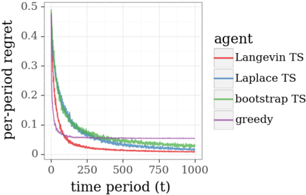
This new model does not enjoy conjugacy properties leveraged in Section 4 and is not amenable to efficient exact Bayesian inference. However, the problem may be addressed via approximation methods. To illustrate, Figure 5.1 plots results from application of three approximate versions of TS to an online shortest path problem on a twenty-stage binomial bridge with binary feedback. The algorithms leverage Langevin Monte Carlo, the Laplace approximation, and the bootstrap, three approaches we will discuss, and the results demonstrate effective learning, in the sense that regret vanishes over time. Also plotted as a baseline for comparison are results from application of the greedy algorithm.
In the remainder of this section, we will describe several approaches to approximate TS. It is worth mentioning that we do not cover an exhaustive list, and further, our descriptions do not serve as comprehensive or definitive treatments of each approach. Rather, our intent is to offer simple descriptions that convey key ideas that may be extended or combined to serve needs arising in any specific application.
Throughout this section, let f t -1 denote the posterior density of θ conditioned on the history H t -1 = (( x 1 , y 1 ) , . . . , ( x t -1 , y t -1 )) of observations. TS generates an action x t by sampling a parameter vector ˆ θ from f t -1 and solving for the optimal path under ˆ θ . The methods we describe generate a sample ˆ θ whose distribution approximates the posterior ˆ f t -1 , which enables approximate implementations of TS when exact posterior sampling is infeasible.
Figure 5.1: Regret experienced by approximation methods applied to the path recommendation problem with binary feedback.
<details>
<summary>Image 9 Details</summary>
### Visual Description
## Line Chart: Per-Period Regret vs. Time Period for Different Agents
### Overview
The image is a line chart comparing the per-period regret of four different agents (Langevin TS, Laplace TS, bootstrap TS, and greedy) over time. The x-axis represents the time period (t), ranging from 0 to 1000. The y-axis represents the per-period regret, ranging from 0 to 0.5. The chart shows how the regret changes over time for each agent.
### Components/Axes
* **Title:** Implicit, but the chart displays "Per-Period Regret vs. Time Period for Different Agents"
* **X-axis:**
* Label: "time period (t)"
* Scale: 0 to 1000, with visible markers at 0, 250, 500, 750, and 1000.
* **Y-axis:**
* Label: "per-period regret"
* Scale: 0 to 0.5, with visible markers at 0, 0.1, 0.2, 0.3, 0.4, and 0.5.
* **Legend:** Located on the right side of the chart.
* "agent"
* Langevin TS (red line)
* Laplace TS (blue line)
* bootstrap TS (green line)
* greedy (purple line)
### Detailed Analysis
* **Langevin TS (red):** The line starts at approximately 0.35 and rapidly decreases to around 0.02 by time period 250. It then fluctuates slightly around this value for the remainder of the time period.
* **Laplace TS (blue):** The line starts at approximately 0.45 and decreases to around 0.04 by time period 500. It then fluctuates slightly around this value for the remainder of the time period.
* **Bootstrap TS (green):** The line starts at approximately 0.5 and decreases to around 0.06 by time period 500. It then fluctuates slightly around this value for the remainder of the time period.
* **Greedy (purple):** The line starts at approximately 0.1 and remains relatively constant around 0.05 for the entire time period.
### Key Observations
* All agents show a decrease in per-period regret over time, but the rate of decrease varies.
* The Langevin TS agent has the lowest per-period regret after the initial decrease.
* The greedy agent has a relatively stable per-period regret throughout the time period.
* The bootstrap TS agent starts with the highest regret, but its regret decreases significantly over time.
### Interpretation
The chart demonstrates the performance of different agents in terms of per-period regret over time. The Langevin TS agent appears to be the most effective in minimizing regret, as it reaches the lowest level and maintains it consistently. The greedy agent, while not achieving the lowest regret, provides a stable performance. The bootstrap TS agent, despite starting with the highest regret, shows a significant improvement over time. The Laplace TS agent performs similarly to the bootstrap TS agent, but its regret decreases at a slower rate. The data suggests that the Langevin TS agent is the preferred choice for minimizing per-period regret in this scenario. The initial rapid decrease in regret for Langevin, Laplace, and Bootstrap TS suggests an initial learning phase, after which the regret stabilizes. The greedy algorithm's flat line suggests it does not adapt or learn over time.
</details>
## 5.1 Gibbs Sampling
Gibbs sampling is a general Markov chain Monte Carlo (MCMC) algorithm for drawing approximate samples from multivariate probability distributions. It produces a sequence of sampled parameters ( ˆ θ n : n = 0 , 1 , 2 , . . . ) forming a Markov chain with stationary distribution f t -1 . Under reasonable technical conditions, the limiting distribution of this Markov chain is its stationary distribution, and the distribution of ˆ θ n converges to f t -1 .
Gibbs sampling starts with an initial guess ˆ θ 0 . Iterating over sweeps n = 1 , . . . , N , for each n th sweep, the algorithm iterates over the components k = 1 , . . . , K , for each k generating a one-dimensional marginal distribution
$$f _ { t - 1 } ^ { n , k } ( \theta _ { k } ) \, \infty \, f _ { t - 1 } ( ( \hat { \theta } _ { 1 } ^ { n } , \dots , \hat { \theta } _ { k - 1 } ^ { n } , \theta _ { k } , \hat { \theta } _ { k + 1 } ^ { n - 1 } , \dots , \hat { \theta } _ { K } ^ { n - 1 } ) ) ,$$
and sampling the k th component according to ˆ θ n k ∼ f n,k t -1 . After N of sweeps, the prevailing vector ˆ θ N is taken to be the approximate posterior sample. We refer to (Casella and George, 1992) for a more thorough introduction to the algorithm.
Gibbs sampling applies to a broad range of problems, and is often computationally viable even when sampling from f t -1 is not. This is because sampling from a one-dimensional distribution is simpler. That
said, for complex problems, Gibbs sampling can still be computationally demanding. This is the case, for example, with our path recommendation problem with binary feedback. In this context, it is easy to implement a version of Gibbs sampling that generates a close approximation to a posterior sample within well under a minute. However, running thousands of simulations each over hundreds of time periods can be quite time-consuming. As such, we turn to more efficient approximation methods.
## 5.2 Laplace Approximation
We now discuss an approach that approximates a potentially complicated posterior distribution by a Gaussian distribution. Samples from this simpler Gaussian distribution can then serve as approximate samples from the posterior distribution of interest. Chapelle and Li (Chapelle and Li, 2011) proposed this method to approximate TS in a display advertising problem with a logistic regression model of ad-click-through rates.
Let g denote a probability density function over R K from which we wish to sample. If g is unimodal, and its log density ln( g ( φ )) is strictly concave around its mode φ , then g ( φ ) = e ln( g ( φ )) is sharply peaked around φ . It is therefore natural to consider approximating g locally around its mode. A second-order Taylor approximation to the log-density gives
$$\ln ( g ( \phi ) ) \approx \ln ( g ( \overline { \phi } ) ) - \frac { 1 } { 2 } ( \phi - \overline { \phi } ) ^ { \top } C ( \phi - \overline { \phi } ) ,$$
$$C = - \nabla ^ { 2 } \ln ( g ( \bar { \phi } ) ) .$$
As an approximation to the density g , we can then use
$$\tilde { g } ( \phi ) \varpropto e ^ { - \frac { 1 } { 2 } ( \phi - \overline { \phi } ) ^ { \top } C ( \phi - \overline { \phi } ) } .$$
This is proportional to the density of a Gaussian distribution with mean φ and covariance C -1 , and hence
$$\tilde { g } ( \phi ) = \sqrt { | C / 2 \pi | } e ^ { - \frac { 1 } { 2 } ( \phi - \overline { \phi } ) ^ { \top } C ( \phi - \overline { \phi } ) } .$$
where
We refer to this as the Laplace approximation of g . Since there are efficient algorithms for generating Gaussian-distributed samples, this offers a viable means to approximately sampling from g .
As an example, let us consider application of the Laplace approximation to Example 5.1. Bayes rule implies that the posterior density f t -1 of θ satisfies
$$f _ { t - 1 } ( \theta ) \varpropto f _ { 0 } ( \theta ) \prod _ { \tau = 1 } ^ { t - 1 } \left ( \frac { 1 } { 1 + \exp \left ( \sum _ { e \in x _ { \tau } } \theta _ { e } - M \right ) } \right ) ^ { y _ { \tau } } \left ( \frac { \exp \left ( \sum _ { e \in x _ { \tau } } \theta _ { e } - M \right ) } { 1 + \exp \left ( \sum _ { e \in x _ { \tau } } \theta _ { e } - M \right ) } \right ) ^ { 1 - y _ { \tau } } .$$
The mode θ can be efficiently computed via maximizing f t -1 , which is log-concave. An approximate posterior sample ˆ θ is then drawn from a Gaussian distribution with mean θ and covariance matrix ( -∇ 2 ln( f t -1 ( θ ))) -1 .
Laplace approximations are well suited for Example 5.1 because the log-posterior density is strictly concave and its gradient and Hessian can be computed efficiently. Indeed, more broadly, Laplace approximations tend to be effective for posterior distributions with smooth densities that are sharply peaked around their mode. They tend to be computationally efficient when one can efficiently compute the posterior mode, and can efficiently form the Hessian of the log-posterior density.
The behavior of the Laplace approximation is not invariant to a substitution of variables, and it can sometimes be helpful to apply such a substitution. To illustrate this point, let us revisit the online shortest path problem of Example 4.2. For this problem, posterior distributions components of θ are log-Gaussian. However, the distribution of φ , where φ e = ln( θ e ) for each edge e ∈ E , is Gaussian. As such, if the Laplace approximation approach is applied to generate a sample ˆ φ from the posterior distribution of φ , the Gaussian approximation is no longer an approximation, and, letting ˆ θ e = exp( ˆ φ e ) for each e ∈ E , we obtain a sample ˆ θ exactly from the posterior distribution of θ . In this case, through a variable substitution, we can sample in a manner that makes the Laplace approximation exact. More broadly, for any given problem, it may be possible to introduce variable substitutions that enhance the efficacy of the Laplace approximation.
To produce the computational results reported in Figure 5.1, we applied Newton's method with a backtracking line search to maximize
ln( f t -1 ). Though regret decays and should eventually vanish, it is easy to see from the figure that, for our example, the performance of the Laplace approximation falls short of Langevin Monte Carlo, which we will discuss in the next section. This is likely due to the fact that the posterior distribution is not sufficiently close to Gaussian. It is interesting that, despite serving as a popular approach in practical applications of TS (Chapelle and Li, 2011; Gómez-Uribe, 2016), the Laplace approximation can leave substantial value on the table.
## 5.3 Langevin Monte Carlo
We now describe an alternative Markov chain Monte Carlo method that uses gradient information about the target distribution. Let g ( φ ) denote a log-concave probability density function over R K from which we wish to sample. Suppose that ln( g ( φ )) is differentiable and its gradients are efficiently computable. Arising first in physics, Langevin dynamics refer to the diffusion process
$$\begin{array} { r l r } { ( 5 . 1 ) } & d \phi _ { t } = \nabla \ln ( g ( \phi _ { t } ) ) d t + \sqrt { 2 } d B _ { t } } \end{array}$$
where B t is a standard Brownian motion process. This process has g as its unique stationary distribution, and under reasonable technical conditions, the distribution of φ t converges rapidly to this stationary distribution (Roberts and Tweedie, 1996; Mattingly et al. , 2002). Therefore simulating the process (5.1) provides a means of approximately sampling from g .
Typically, one instead implements a Euler discretization of this stochastic differential equation
$$\phi _ { n + 1 } = \phi _ { n } + \epsilon \nabla \ln ( g ( \phi _ { n } ) ) + \sqrt { 2 \epsilon } W _ { n } \quad n \in \mathbb { N } ,$$
where W 1 , W 2 , . . . are i.i.d. standard Gaussian random variables and /epsilon1 > 0 is a small step size. Like a gradient ascent method, under this method φ n tends to drift in directions of increasing density g ( φ n ). However, random Gaussian noise W n is injected at each step so that, for large n , the position of φ n is random and captures the uncertainty in the distribution g . A number of papers establish rigorous guarantees for the rate at which this Markov chain converges to its stationary
distribution (Roberts and Rosenthal, 1998; Bubeck et al. , 2018; Durmus and Moulines, 2016; Cheng and Bartlett, 2018). These papers typically require /epsilon1 is sufficiently small, or that a decaying sequence of step sizes ( /epsilon1 1 , /epsilon1 2 , . . . ) is used.
We make two standard modifications to this method to improve computational efficiency. First, following recent work (Welling and Teh, 2011), we implement stochastic gradient Langevin Monte Carlo, which uses sampled minibatches of data to compute approximate rather than exact gradients. Our implementation uses a mini-batch size of 100; this choice seems to be effective but has not been carefully optimized. When fewer than 100 observations are available, we follow the Markov chain (5.2) with exact gradient computation. When more than 100 observations have been gathered, we follow (5.2) but use an estimated gradient ∇ ln(ˆ g n ( φ n )) at each step based on a random subsample of 100 data points. Some work provides rigorous guarantees for stochastic gradient Langevin Monte Carlo by arguing the cumulative impact of the noise in gradient estimation is second order relative to the additive Gaussian noise (Teh et al. , 2016).
Our second modification involves the use of a preconditioning matrix to improve the mixing rate of the Markov chain (5.2). For the path recommendation problem in Example 5.1, we have found that the log posterior density becomes ill-conditioned in later time periods. For this reason, gradient ascent converges very slowly to the posterior mode. Effective optimization methods should leverage second order information. Similarly, due to poor conditioning, we may need to choose an extremely small step size /epsilon1 , causing the Markov chain in 5.2 to mix slowly. We have found that preconditioning substantially improves performance. Langevin MCMC can be implemented with a symmetric positive definite preconditioning matrix A by simulating the Markov chain
$$\begin{array} { r l } & { \phi _ { n + 1 } = \phi _ { n } + \epsilon A \nabla \ln ( g ( \phi _ { n } ) ) + \sqrt { 2 } \epsilon A ^ { 1 / 2 } W _ { n } \quad n \in \mathbb { N } , } \end{array}$$
where A 1 / 2 denotes the matrix square root of A . In our implementation, we take φ 0 = argmax φ ln( g ( φ )), so the chain is initialized at the posterior mode, computed via means discussed in Section 5.2, and take the preconditioning matrix A = -( ∇ 2 ln( g ( φ )) | φ = φ 0 ) -1 to be the negative inverse Hessian at that point. It may be possible to improve
computational efficiency by constructing an incremental approximation to the Hessian, as we will discuss in Subsection 5.6, but we do not explore that improvement here.
## 5.4 Bootstrapping
As an alternative, we discuss an approach based on the statistical bootstrap, which accommodates even very complex densities. Use of the bootstrap for TS was first considered in (Eckles and Kaptein, 2014), though the version studied there applies to Bernoulli bandits and does not naturally generalize to more complex problems. There are many other versions of the bootstrap approach that can be used to approximately sample from a posterior distribution. For concreteness, we introduce a specific one that is suitable for examples we cover in this tutorial.
Like the Laplace approximation approach, our bootstrap method assumes that θ is drawn from a Euclidean space R K . Consider first a standard bootstrap method for evaluating the sampling distribution of the maximum likelihood estimate of θ . The method generates a hypothetical history ˆ H t -1 = ((ˆ x 1 , ˆ y 1 ) , . . . , (ˆ x t -1 , ˆ y t -1 )), which is made up of t -1 action-observation pairs, each sampled uniformly with replacement from H t -1 . We then maximize the likelihood of θ under the hypothetical history, which for our shortest path recommendation problem is given by
$$\begin{array} { r } { \hat { L } _ { t - 1 } ( \theta ) = \prod _ { \tau = 1 } ^ { t - 1 } \left ( \frac { 1 } { 1 + \exp \left ( \sum _ { e \in \hat { x } _ { \tau } } \theta _ { e } - M \right ) } \right ) ^ { \hat { y } _ { \tau } } \left ( \frac { \exp \left ( \sum _ { e \in \hat { x } _ { \tau } } \theta _ { e } - M \right ) } { 1 + \exp \left ( \sum _ { e \in \hat { x } _ { \tau } } \theta _ { e } - M \right ) } \right ) ^ { 1 - \hat { y } _ { \tau } } . } \end{array}$$
The randomness in the maximizer of ˆ L t -1 reflects the randomness in the sampling distribution of the maximum likelihood estimate. Unfortunately, this method does not take the agent's prior into account. A more severe issue is that it grossly underestimates the agent's real uncertainty in initial periods. The modification described here is intended to overcome these shortcomings in a simple way.
The method proceeds as follows. First, as before, we draw a hypothetical history ˆ H t -1 = ((ˆ x 1 , ˆ y 1 ) , . . . , (ˆ x t -1 , ˆ y t -1 )), which is made up of t -1 action-observation pairs, each sampled uniformly with replacement
from H t -1 . Next, we draw a sample θ 0 from the prior distribution f 0 . Let Σ denote the covariance matrix of the prior f 0 . Finally, we solve the maximization problem
$$\hat { \theta } = \underset { \theta \in \mathbb { R } ^ { k } } { \arg \max } \ e ^ { - ( \theta - \theta ^ { 0 } ) ^ { \top } \Sigma ( \theta - \theta ^ { 0 } ) } \hat { L } _ { t - 1 } ( \theta )$$
and treat ˆ θ as an approximate posterior sample. This can be viewed as maximizing a randomized approximation ˆ f t -1 to the posterior density, where ˆ f t -1 ( θ ) ∝ e -( θ -θ 0 ) /latticetop Σ( θ -θ 0 ) ˆ L t -1 ( θ ) is what the posterior density would be if the prior were Gaussian with mean θ 0 and covariance matrix Σ, and the history of observations were ˆ H t -1 . When very little data has been gathered, the randomness in the samples mostly stems from the randomness in the prior sample θ 0 . This random prior sample encourages the agent to explore in early periods. When t is large, so a lot of a data has been gathered, the likelihood typically overwhelms the prior sample and randomness in the samples mostly stems from the random selection of the history ˆ H t -1 .
In the context of the shortest path recommendation problem, ˆ f t -1 ( θ ) is log-concave and can therefore be efficiently maximized. Again, to produce our computational results reported in Figure 5.1, we applied Newton's method with a backtracking line search to maximize ln( ˆ f t -1 ). Even when it is not possible to efficiently maximize ˆ f t -1 , however, the bootstrap approach can be applied with heuristic optimization methods that identify local or approximate maxima.
As can be seen from Figure 5.1, for our example, bootstrapping performs about as well as the Laplace approximation. One advantage of the bootstrap is that it is nonparametric, and may work reasonably regardless of the functional form of the posterior distribution, whereas the Laplace approximation relies on a Gaussian approximation and Langevin Monte Carlo relies on log-concavity and other regularity assumptions. That said, it is worth mentioning that there is a lack of theoretical justification for bootstrap approaches or even understanding of whether there are nontrivial problem classes for which they are guaranteed to perform well.
## 5.5 Sanity Checks
Figure 5.1 demonstrates that Laplace approximation, Langevin Monte Carlo, and bootstrap approaches, when applied to the path recommendation problem, learn from binary feedback to improve performance over time. This may leave one wondering, however, whether exact TS would offer substantially better performance. Since we do not have a tractable means of carrying out exact TS for this problem, in this section, we apply our approximation methods to problems for which exact TS is tractable. This enables comparisons between performance of exact and approximate methods.
Recall the three-armed beta-Bernoulli bandit problem for which results from application of greedy and TS algorithms were reported in Figure 3.2(b). For this problem, components of θ are independent under posterior distributions, and as such, Gibbs sampling yields exact posterior samples. Hence, the performance of an approximate version that uses Gibbs sampling would be identical to that of exact TS. Figure 5.2a plots results from applying Laplace approximation, Langevin Monte Carlo, and bootstrap approaches. For this problem, our approximation methods offer performance that is qualitatively similar to exact TS, though the Laplace approximation performs marginally worse than alternatives in this setting.
Next, consider the online shortest path problem with correlated edge delays. Regret experienced by TS applied to such a problem were reported in Figure 4.3a. As discussed in Section 5.2, applying the Laplace approximation approach with an appropriate variable substitution leads to the same results as exact TS. Figure 5.2b compares those results to what is generated by Gibbs sampling, Langevin Monte Carlo, and bootstrap approaches. Again, the approximation methods yield competitive results, although bootstrapping is marginally less effective than others.
It is easy to verify that for the online shortest path problem and specific choices of step size /epsilon1 = 1 / 2 and conditioning matrix A = Σ t , a single Langevin Monte Carlo iteration offers an exact posterior sample. However, our simulations do not use this step size and carry out multiple iterations. The point here is not to optimize results for our specific problem but rather to offer a sanity check for the approach.
Figure 5.2: Regret of approximation methods versus exact Thompson sampling.
<details>
<summary>Image 10 Details</summary>
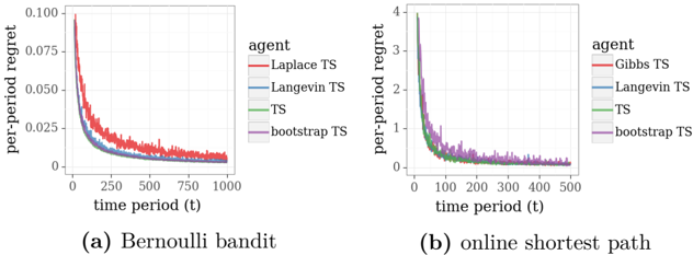
### Visual Description
## Chart: Per-Period Regret vs. Time Period for Different Agents
### Overview
The image contains two line charts comparing the per-period regret of different agents over time. The left chart (a) shows results for a Bernoulli bandit problem, while the right chart (b) shows results for an online shortest path problem. Both charts display the per-period regret on the y-axis and the time period (t) on the x-axis. The performance of four different agents (Laplace TS/Gibbs TS, Langevin TS, TS, and bootstrap TS) are compared in each chart.
### Components/Axes
**Left Chart (a) Bernoulli bandit:**
* **Title:** (a) Bernoulli bandit
* **X-axis:** time period (t), ranging from 0 to 1000
* **Y-axis:** per-period regret, ranging from 0 to 0.100
* **Legend (top-right):**
* Red: Laplace TS
* Blue: Langevin TS
* Green: TS
* Purple: bootstrap TS
**Right Chart (b) online shortest path:**
* **Title:** (b) online shortest path
* **X-axis:** time period (t), ranging from 0 to 500
* **Y-axis:** per-period regret, ranging from 0 to 4
* **Legend (top-right):**
* Red: Gibbs TS
* Blue: Langevin TS
* Green: TS
* Purple: bootstrap TS
### Detailed Analysis
**Left Chart (a) Bernoulli bandit:**
* **Laplace TS (Red):** The per-period regret starts at approximately 0.1 and decreases rapidly, reaching approximately 0.02 around time period 250, then gradually decreases to approximately 0.01 by time period 1000.
* **Langevin TS (Blue):** The per-period regret starts at approximately 0.05 and decreases rapidly, reaching approximately 0.01 around time period 250, then remains relatively stable.
* **TS (Green):** The per-period regret starts at approximately 0.075 and decreases rapidly, reaching approximately 0.01 around time period 250, then remains relatively stable.
* **bootstrap TS (Purple):** The per-period regret starts at approximately 0.075 and decreases rapidly, reaching approximately 0.01 around time period 250, then remains relatively stable.
**Right Chart (b) online shortest path:**
* **Gibbs TS (Red):** The per-period regret starts at approximately 4 and decreases rapidly, reaching approximately 0.5 around time period 100, then gradually decreases to approximately 0.2 by time period 500.
* **Langevin TS (Blue):** The per-period regret starts at approximately 2 and decreases rapidly, reaching approximately 0.25 around time period 100, then remains relatively stable.
* **TS (Green):** The per-period regret starts at approximately 3 and decreases rapidly, reaching approximately 0.5 around time period 100, then remains relatively stable.
* **bootstrap TS (Purple):** The per-period regret starts at approximately 2 and decreases rapidly, reaching approximately 0.5 around time period 100, then remains relatively stable.
### Key Observations
* In both charts, all agents exhibit a rapid decrease in per-period regret during the initial time periods.
* In the Bernoulli bandit problem, the Laplace TS agent initially has a higher regret but converges to a similar level as the other agents.
* In the online shortest path problem, the Gibbs TS agent initially has a higher regret but converges to a higher level than the other agents.
* The Langevin TS, TS, and bootstrap TS agents show similar performance in both problems after the initial rapid decrease in regret.
### Interpretation
The charts demonstrate the learning behavior of different Thompson Sampling (TS) based agents in two different problem settings: Bernoulli bandit and online shortest path. The initial rapid decrease in per-period regret indicates that all agents are effectively learning to make better decisions over time. The differences in initial regret and convergence levels suggest that the choice of agent can impact performance, particularly in the early stages of learning. The Laplace TS and Gibbs TS agents, which use different sampling strategies, exhibit distinct behaviors compared to the other agents. The Langevin TS, TS, and bootstrap TS agents show relatively consistent performance across both problem settings, suggesting that they are robust to changes in the environment.
</details>
## 5.6 Incremental Implementation
For each of the three approximation methods we have discussed, the computation time required per time period grows as time progresses. This is because each past observation must be accessed to generate the next action. This differs from exact TS algorithms we discussed earlier, which maintain parameters that encode a posterior distribution, and update these parameters over each time period based only on the most recent observation.
In order to keep the computational burden manageable, it can be important to consider incremental variants of our approximation methods. We refer to an algorithm as incremental if it operates with fixed rather than growing per-period compute time. There are many ways to design incremental variants of approximate posterior sampling algorithms we have presented. As concrete examples, we consider here particular incremental versions of Laplace approximation and bootstrap approaches.
For each time t , let /lscript t ( θ ) denote the likelihood of y t conditioned on x t and θ . Hence, conditioned on H t -1 , the posterior density satisfies
$$f _ { t - 1 } ( \theta ) \varpropto f _ { 0 } ( \theta ) \prod _ { \tau = 1 } ^ { t - 1 } \ell _ { \tau } ( \theta ) .$$
Let g 0 ( θ ) = ln( f 0 ( θ )) and g t ( θ ) = ln( /lscript t ( θ )) for t > 0. To identify the mode of f t -1 , it suffices to maximize ∑ t -1 τ =0 g τ ( θ ).
Consider an incremental version of the Laplace approximation. The algorithm maintains statistics H t , and θ t , initialized with θ 0 = argmax θ g 0 ( θ ), and H 0 = ∇ 2 g 0 ( θ 0 ), and updating according to
$$H _ { t } = H _ { t - 1 } + \nabla ^ { 2 } g _ { t } ( \overline { \theta } _ { t - 1 } ) , \\ \bar { \theta } _ { t } = \bar { \theta } _ { t - 1 } - H _ { t } ^ { - 1 } \nabla g _ { t } ( \overline { \theta } _ { t - 1 } ) .$$
This algorithm is a type of online newton method for computing the posterior mode θ t -1 that maximizes ∑ t -1 τ =0 g τ ( θ ). Note that if each function g t -1 is strictly concave and quadratic, as would be the case if the prior is Gaussian and observations are linear in θ and perturbed only by Gaussian noise, each pair θ t -1 and H -1 t -1 represents the mean and covariance matrix of f t -1 . More broadly, these iterates can be viewed as the mean and covariance matrix of a Gaussian approximation to the posterior, and used to generate an approximate posterior sample ˆ θ ∼ N ( θ t -1 , H -1 t -1 ). It is worth noting that for linear and generalized linear models, the matrix ∇ 2 g t ( θ t -1 ) has rank one, and therefore H -1 t = ( H t -1 + ∇ 2 g t ( θ t -1 )) -1 can be updated incrementally using the Sherman-Woodbury-Morrison formula. This incremental version of the Laplace approximation is closely related to the notion of an extended Kalman filter, which has been explored in greater depth by Gómez-Uribe (Gómez-Uribe, 2016) as a means for incremental approximate TS with exponential families of distributions.
Another approach involves incrementally updating each of an ensemble of models to behave like a sample from the posterior distribution. The posterior can be interpreted as a distribution of 'statistically plausible' models, by which we mean models that are sufficiently consistent with prior beliefs and the history of observations. With this interpretation in mind, TS can be thought of as randomly drawing from the range of statistically plausible models. Ensemble sampling aims to maintain, incrementally update, and sample from a finite set of such models. In the spirit of particle filtering, this set of models approximates the posterior distribution. The workings of ensemble sampling are in some ways more intricate than conventional uses of particle filtering, however, because interactions between the ensemble of models and selected actions can skew the distribution. Ensemble sampling is presented in more depth
in (Lu and Van Roy, 2017), which draws inspiration from work on exploration in deep reinforcement learning (Osband et al. , 2016a).
There are multiple ways of generating suitable model ensembles. One builds on the aforementioned bootstrap method and involves fitting each model to a different bootstrap sample. To elaborate, consider maintaining N models with parameters ( θ n t , H n t : n = 1 , . . . , N ). Each set is initialized with θ n 0 ∼ g 0 , H n 0 = ∇ g 0 ( θ n 0 ), d n 0 = 0, and updated according to
$$7 2$$
$$& H _ { t } ^ { n } = H _ { t - 1 } ^ { n } + z _ { t } ^ { n } \nabla ^ { 2 } g _ { t } ( \overline { \theta } _ { t - 1 } ^ { n } ) , \\ & \overline { \theta } _ { t } ^ { n } = \overline { \theta } _ { t - 1 } ^ { n } - z _ { t } ^ { n } ( H _ { t } ^ { n } ) ^ { - 1 } \nabla g _ { t } ( \overline { \theta } _ { t - 1 } ^ { n } ) ,$$
$$3$$
where each z n t is an independent Poisson-distributed sample with mean one. Each θ n t can be viewed as a random statistically plausible model, with randomness stemming from the initialization of θ n 0 and the random weight z n t placed on each observation. The variable, z n τ can loosely be interpreted as a number of replicas of the data sample ( x τ , y τ ) placed in a hypothetical history ˆ H n t . Indeed, in a data set of size t , the number of replicas of a particular bootstrap data sample follows a Binomial( t, 1 /t ) distribution, which is approximately Poisson(1) when t is large. With this view, each θ n t is effectively fit to a different data set ˆ H n t , distinguished by the random number of replicas assigned to each data sample. To generate an action x t , n is sampled uniformly from { 1 , . . . , N } , and the action is chosen to maximize E [ r t | θ = θ n t -1 ]. Here, θ n t -1 serves as the approximate posterior sample. Note that the per-period compute time grows with N , which is an algorithm tuning parameter.
This bootstrap approach offers one mechanism for incrementally updating an ensemble of models. In Section 7.4, we will discuss another, which we apply to active learning with neural networks.
## Practical Modeling Considerations
Our narrative over previous sections has centered around a somewhat idealized view of TS, which ignored the process of prior specification and assumed a simple model in which the system and set of feasible actions is constant over time and there is no side information on decision context. In this section, we provide greater perspective on the process of prior specification and on extensions of TS that serve practical needs arising in some applications.
## 6.1 Prior Distribution Specification
The algorithms we have presented require as input a prior distribution over model parameters. The choice of prior can be important, so let us now discuss its role and how it might be selected. In designing an algorithm for an online decision problem, unless the value of θ were known with certainty, it would not make sense to optimize performance for a single value, because that could lead to poor performance for other plausible values. Instead, one might design the algorithm to perform well on average across a collection of possibilities. The prior can be thought of as a distribution over plausible values, and its choice directs
the algorithm to perform well on average over random samples from the prior.
For a practical example of prior selection, let us revisit the banner ad placement problem introduced in Example 1.1. There are K banner ads for a single product, with unknown click-through probabilities ( θ 1 , . . . , θ K ). Given a prior, TS can learn to select the most successful ad. We could use a uniform or, equivalently, a beta(1 , 1) distribution over each θ k . However, if some values of θ k are more likely than others, using a uniform prior sacrifices performance. In particular, this prior represents no understanding of the context, ignoring any useful knowledge from past experience. Taking knowledge into account reduces what must be learned and therefore reduces the time it takes for TS to identify the most effective ads.
Suppose we have a data set collected from experience with previous products and their ads, each distinguished by stylistic features such as language, font, and background, together with accurate estimates of click-through probabilities. Let us consider an empirical approach to prior selection that leverages this data. First, partition past ads into K sets, with each k th partition consisting of those with stylistic features most similar to the k th ad under current consideration. Figure 6.1 plots a hypothetical empirical cumulative distribution of click-through probabilities for ads in the k th set. It is then natural to consider as a prior a smoothed approximation of this distribution, such as the beta(1 , 100) distribution also plotted in Figure 6.1. Intuitively, this process assumes that click-through probabilities of past ads in set k represent plausible values of θ k . The resulting prior is informative; among other things, it virtually rules out click-through probabilities greater than 0 . 05.
A careful choice of prior can improve learning performance. Figure 6.2 presents results from simulations of a three-armed Bernoulli bandit. Mean rewards of the three actions are sampled from beta(1 , 50), beta(1 , 100), and beta(1 , 200) distributions, respectively. TS is applied with these as prior distributions and with a uniform prior distribution. We refer to the latter as a misspecified prior because it is not consistent with our understanding of the problem. A prior that is consistent in this sense is termed coherent . Each plot represents an average over ten thousand independent simulations, each with independently sampled
Figure 6.1: An empirical cumulative distribution and an approximating beta distribution.
<details>
<summary>Image 11 Details</summary>
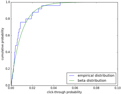
### Visual Description
## Chart: Cumulative Distribution of Click-Through Probability
### Overview
The image is a chart comparing the cumulative distribution of click-through probability for an empirical distribution and a beta distribution. The x-axis represents click-through probability, and the y-axis represents cumulative probability.
### Components/Axes
* **X-axis:** "click-through probability" with scale from 0.00 to 0.10 in increments of 0.02.
* **Y-axis:** "cumulative probability" with scale from 0.0 to 1.0 in increments of 0.2.
* **Legend:** Located in the bottom-right corner.
* Blue line: "empirical distribution"
* Green line: "beta distribution"
### Detailed Analysis
* **Empirical Distribution (Blue):** The empirical distribution is represented by a step function.
* At x=0.00, y=0.00
* At x=0.005 (approximately), y=0.08
* At x=0.01, y=0.25
* At x=0.015, y=0.40
* At x=0.02, y=0.55
* At x=0.025, y=0.70
* At x=0.03, y=0.78
* At x=0.035, y=0.90
* At x=0.04, y=0.95
* At x=0.05, y=0.98
* At x=0.10, y=1.00
The empirical distribution rises sharply initially and then gradually approaches 1.0.
* **Beta Distribution (Green):** The beta distribution is represented by a smooth curve.
* At x=0.00, y=0.00
* At x=0.005, y=0.25
* At x=0.01, y=0.45
* At x=0.015, y=0.60
* At x=0.02, y=0.70
* At x=0.025, y=0.78
* At x=0.03, y=0.85
* At x=0.035, y=0.90
* At x=0.04, y=0.93
* At x=0.05, y=0.97
* At x=0.10, y=1.00
The beta distribution also rises sharply initially and then gradually approaches 1.0, but it is smoother than the empirical distribution.
### Key Observations
* Both distributions show a rapid increase in cumulative probability for small values of click-through probability.
* The empirical distribution has a stepped appearance due to the discrete nature of the data.
* The beta distribution provides a smoothed representation of the cumulative probability.
* The beta distribution appears to be a good fit for the empirical distribution.
### Interpretation
The chart compares the cumulative distribution of click-through probabilities from an empirical dataset to a theoretical beta distribution. The empirical distribution represents the actual observed click-through rates, while the beta distribution is a model that attempts to fit the observed data. The close alignment of the two distributions suggests that the beta distribution is a reasonable model for the observed click-through probabilities. This can be useful for predicting future click-through rates or for comparing the performance of different advertising campaigns. The initial sharp rise in both distributions indicates that a large proportion of clicks occur at very low click-through probabilities.
</details>
mean rewards. Figure 6.2a plots expected regret, demonstrating that the misspecified prior increases regret. Figure 6.2a plots the evolution of the agent's mean reward conditional expectations. For each algorithm, there are three curves corresponding to the best, second-best, and worst actions, and they illustrate how starting with a misspecified prior delays learning.
Figure 6.2: Comparison of TS for the Bernoulli bandit problem with coherent versus misspecified priors.
<details>
<summary>Image 12 Details</summary>
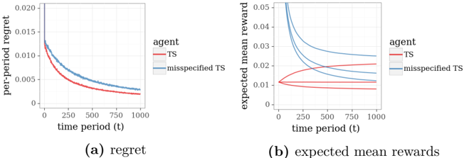
### Visual Description
## Chart: Regret and Expected Mean Rewards Comparison
### Overview
The image presents two line charts comparing the performance of two agents, "TS" (Thompson Sampling) and "misspecified TS," over time. The left chart (a) displays the per-period regret, while the right chart (b) shows the expected mean reward. Both charts share the same x-axis representing "time period (t)" from 0 to 1000.
### Components/Axes
**Chart (a): Regret**
* **Y-axis:** "per-period regret," ranging from 0 to 0.020 with increments of 0.005.
* **X-axis:** "time period (t)," ranging from 0 to 1000 with increments of 250.
* **Legend (top-right):**
* Red line: "TS"
* Blue line: "misspecified TS"
**Chart (b): Expected Mean Rewards**
* **Y-axis:** "expected mean reward," ranging from 0 to 0.05 with increments of 0.01.
* **X-axis:** "time period (t)," ranging from 0 to 1000 with increments of 250.
* **Legend (top-right):**
* Red line: "TS"
* Blue line: "misspecified TS"
### Detailed Analysis
**Chart (a): Regret**
* **TS (Red):** The per-period regret starts at approximately 0.012 and decreases over time, approaching a value around 0.002 after 1000 time periods. The decline is steeper initially and then flattens out.
* **Misspecified TS (Blue):** The per-period regret starts at approximately 0.014 and also decreases over time, approaching a value around 0.004 after 1000 time periods. The decline is steeper initially and then flattens out. The regret for misspecified TS is consistently higher than that of TS.
**Chart (b): Expected Mean Rewards**
* **TS (Red):** There are two red lines. One starts at approximately 0.012 and decreases slightly to around 0.011. The other starts at approximately 0.01 and increases slightly to around 0.012.
* **Misspecified TS (Blue):** There are two blue lines. One starts at approximately 0.01 and increases sharply to approximately 0.025, then increases more slowly to approximately 0.027. The other starts at approximately 0.05 and decreases sharply to approximately 0.02, then decreases more slowly to approximately 0.017.
### Key Observations
* In the regret chart, both agents show a decreasing trend in per-period regret over time, with the "TS" agent consistently exhibiting lower regret than the "misspecified TS" agent.
* In the expected mean rewards chart, the "TS" agent's reward remains relatively stable, while the "misspecified TS" agent's reward shows more significant fluctuations, with one line increasing and the other decreasing.
### Interpretation
The data suggests that the "TS" agent performs better in terms of minimizing regret compared to the "misspecified TS" agent. The "TS" agent also demonstrates more stable expected mean rewards. The "misspecified TS" agent, while initially having higher expected mean rewards, experiences more volatility and ultimately converges to a lower reward level than its initial peak. This indicates that the "TS" agent is more robust and efficient in this scenario. The "misspecified TS" agent's performance is likely affected by the model misspecification, leading to higher regret and unstable rewards.
</details>
## 6.2 Constraints, Context, and Caution
Though Algorithm 4.2, as we have presented it, treats a very general model, straightforward extensions accommodate even broader scope. One involves imposing time-varying constraints on the actions. In particular, there could be a sequence of admissible action sets X t that constrain actions x t . To motivate such an extension, consider our shortest path example. Here, on any given day, the drive to work may be constrained by announced road closures. If X t does not depend on θ except through possible dependence on the history of observations, TS (Algorithm 4.2) remains an effective approach, with the only required modification being to constrain the maximization problem in Line 6.
Another extension of practical import addresses contextual online decision problems . In such problems, the response y t to action x t also depends on an independent random variable z t that the agent observes prior to making her decision. In such a setting, the conditional distribution of y t takes the form p θ ( ·| x t , z t ). To motivate this, consider again the shortest path example, but with the agent observing a weather report z t from a news channel before selecting a path x t . Weather may affect delays along different edges differently, and the agent can take this into account before initiating her trip. Contextual problems of this flavor can be addressed through augmenting the action space and introducing time-varying constraint sets. In particular, if we view ˜ x t = ( x t , z t ) as the action and constrain its choice to X t = { ( x, z t ) : x ∈ X} , where X is the set from which x t must be chosen, then it is straightforward to apply TS to select actions ˜ x 1 , ˜ x 2 , . . . . For the shortest path problem, this can be interpreted as allowing the agent to dictate both the weather report and the path to traverse, but constraining the agent to provide a weather report identical to the one observed through the news channel.
In some applications, it may be important to ensure that expected performance exceeds some prescribed baseline. This can be viewed as a level of caution against poor performance. For example, we might want each action applied to offer expected reward of at least some level r . This can again be accomplished through constraining actions: in each t th time period, let the action set be X t = { x ∈ X : E [ r t | x t = x ] ≥ r } . Using such an action set ensures that expected average reward exceeds
r . When actions are related, an actions that is initially omitted from the set can later be included if what is learned through experiments with similar actions increases the agent's expectation of reward from the initially omitted action.
## 6.3 Nonstationary Systems
Problems we have considered involve model parameters θ that are constant over time. As TS hones in on an optimal action, the frequency of exploratory actions converges to zero. In many practical applications, the agent faces a nonstationary system, which is more appropriately modeled by time-varying parameters θ 1 , θ 2 , . . . , such that the response y t to action x t is generated according to p θ t ( ·| x t ). In such contexts, the agent should never stop exploring, since it needs to track changes as the system drifts. With minor modification, TS remains an effective approach so long as model parameters change little over durations that are sufficient to identify effective actions.
In principle, TS could be applied to a broad range of problems where the parameters θ 1 , θ 2 , θ 3 , ... evolve according to a stochastic process by using techniques from filtering and sequential Monte Carlo to generate posterior samples. Instead we describe below some much simpler approaches to such problems.
One simple approach to addressing nonstationarity involves ignoring historical observations made beyond some number τ of time periods in the past. With such an approach, at each time t , the agent would produce a posterior distribution based on the prior and conditioned only on the most recent τ actions and observations. Model parameters are sampled from this distribution, and an action is selected to optimize the associated model. The agent never ceases to explore, since the degree to which the posterior distribution can concentrate is limited by the number of observations taken into account. Theory supporting such an approach is developed in (Besbes et al. , 2014).
An alternative approach involves modeling evolution of a belief distribution in a manner that discounts the relevance of past observations and tracks a time-varying parameters θ t . We now consider such a model and a suitable modification of TS. Let us start with
the simple context of a Bernoulli bandit. Take the prior for each k th mean reward to be beta( α, β ). Let the algorithm update parameters to identify the belief distribution of θ t conditioned on the history H t -1 = (( x 1 , y 1 ) , . . . , ( x t -1 , y t -1 )) according to (6.1)
/negationslash
$$\begin{array} { r } { ( \alpha _ { k } , \beta _ { k } ) \leftarrow \left \{ \begin{array} { l l } { \left ( ( 1 - \gamma ) \alpha _ { k } + \gamma \overline { \alpha } , ( 1 - \gamma ) \beta _ { k } + \gamma \overline { \beta } \right ) } & { x _ { t } \neq k } \\ { \left ( ( 1 - \gamma ) \alpha _ { k } + \gamma \overline { \alpha } + r _ { t } , ( 1 - \gamma ) \beta _ { k } + \gamma \overline { \beta } + 1 - r _ { t } \right ) } & { x _ { t } = k , } \end{array} } \end{array}$$
where γ ∈ [0 , 1] and α k , β k > 0. This models a process for which the belief distribution converges to beta( α k , β k ) in the absence of observations. Note that, in the absence of observations, if γ > 0 then ( α k , β k ) converges to ( α k , β k ). Intuitively, the process can be thought of as randomly perturbing model parameters in each time period, injecting uncertainty. The parameter γ controls how quickly uncertainty is injected. At one extreme, when γ = 0, no uncertainty is injected. At the other extreme, γ = 1 and each θ t,k is an independent beta( α k , β k )-distributed process. A modified version of Algorithm 3.2 can be applied to this nonstationary Bernoulli bandit problem, the differences being in the additional arguments γ , α , and β , and the formula used to update distribution parameters.
The more general form of TS presented in Algorithm 4.2 can be modified in an analogous manner. For concreteness, let us focus on the case where θ is restricted to a finite set; it is straightforward to extend things to infinite sets. The conditional distribution update in Algorithm 4.2 can be written as
$$p ( u ) \leftarrow \frac { p ( u ) q _ { u } ( y _ { t } | x _ { t } ) } { \sum _ { v } p ( v ) q _ { v } ( y _ { t } | x _ { t } ) } .$$
To model nonstationary model parameters, we can use the following alternative:
$$p ( u ) \leftarrow \frac { \overline { p } ^ { \gamma } ( u ) p ^ { 1 - \gamma } ( u ) q _ { u } ( y _ { t } | x _ { t } ) } { \sum _ { v } \overline { p } ^ { \gamma } ( v ) p ^ { 1 - \gamma } ( v ) q _ { v } ( y _ { t } | x _ { t } ) } .$$
This generalizes the formula provided earlier for the Bernoulli bandit case. Again, γ controls the rate at which uncertainty is injected. The modified version of Algorithm 3.2, which we refer to as nonstationary TS , takes γ and p as additional arguments and replaces the distribution update formula.
Figure 6.3 illustrates potential benefits of nonstationary TS when dealing with a nonstationairy Bernoulli bandit problem. In these simulations, belief distributions evolve according to Equation (6.1). The prior and stationary distributions are specified by α = α = β = β = 1. The decay rate is γ = 0 . 01. Each plotted point represents an average over 10,000 independent simulations. Regret here is defined by regret t ( θ t ) = max k θ t,k -θ t,x t . While nonstationary TS updates its belief distribution in a manner consistent with the underlying system, TS pretends that the success probabilities are constant over time and updates its beliefs accordingly. As the system drifts over time, TS becomes less effective, while nonstationary TS retains reasonable performance. Note, however, that due to nonstationarity, no algorithm can promise regret that vanishes with time.
Figure 6.3: Comparison of TS versus nonstationary TS with a nonstationary Bernoulli bandit problem.
<details>
<summary>Image 13 Details</summary>
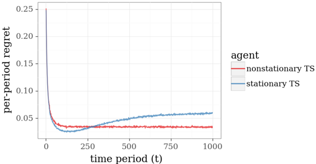
### Visual Description
## Line Chart: Per-Period Regret vs. Time Period for Different Agents
### Overview
The image is a line chart comparing the per-period regret of two agents, "nonstationary TS" and "stationary TS", over time. The x-axis represents the time period (t), ranging from 0 to 1000. The y-axis represents the per-period regret, ranging from 0 to 0.25. The chart displays how the regret changes for each agent over the specified time period.
### Components/Axes
* **X-axis:** "time period (t)" with tick marks at 0, 250, 500, 750, and 1000.
* **Y-axis:** "per-period regret" with tick marks at 0, 0.05, 0.10, 0.15, 0.20, and 0.25.
* **Legend (top-right):**
* "agent"
* Red line: "nonstationary TS"
* Blue line: "stationary TS"
### Detailed Analysis
* **Nonstationary TS (Red Line):**
* Starts at approximately 0.25 at time period 0.
* Decreases rapidly to approximately 0.03 by time period 100.
* Remains relatively stable around 0.03 to 0.04 from time period 100 to 1000.
* **Stationary TS (Blue Line):**
* Starts at approximately 0.25 at time period 0.
* Decreases rapidly to approximately 0.03 by time period 100.
* Increases gradually from approximately 0.03 at time period 100 to approximately 0.06 at time period 1000.
### Key Observations
* Both agents exhibit a sharp decrease in per-period regret initially.
* The nonstationary TS agent maintains a consistently low regret level after the initial drop.
* The stationary TS agent's regret increases gradually over time after the initial drop.
* The stationary TS agent's regret surpasses the nonstationary TS agent's regret after approximately time period 250.
### Interpretation
The chart suggests that the nonstationary TS agent is more effective in maintaining a low per-period regret over the long term compared to the stationary TS agent. While both agents initially perform similarly, the stationary TS agent's performance degrades over time, leading to a higher regret. This could be due to the nonstationary TS agent's ability to adapt to changing conditions, while the stationary TS agent is optimized for a fixed environment. The initial rapid decrease in regret for both agents indicates a quick learning phase, after which the nonstationary TS agent continues to refine its strategy, while the stationary TS agent plateaus.
</details>
## 6.4 Concurrence
In many applications, actions are applied concurrently. As an example, consider a variation of the online shortest path problem of Example 4.1. In the original version of this problem, over each period, an agent selects and traverses a path from origin to destination, and upon completion, updates a posterior distribution based on observed edge traversal times.
Now consider a case in which, over each period, multiple agents travel between the same origin and destination, possibly along different paths, with the travel time experienced by agents along each edge e to conditionally independent, conditioned on θ e . At the end of the period, agents update a common posterior distribution based on their collective experience. The paths represent concurrent actions, which should be selected in a manner that diversifies experience.
TS naturally suits this concurrent mode of operation. Given the posterior distribution available at the beginning of a time period, multiple independent samples can be drawn to produce paths for multiple agents. Figure 6.4 plots results from applying TS in this manner. Each simulation was carried out with K agents navigating over each time period through a twenty-stage binomial bridge. Figure 6.4(a) demonstrates that the per-action regret experienced by each agent decays more rapidly with time as the number of agents grows. This is due to the fact that each agent's learning is accelerated by shared observations. On the other hand, Figure 6.4(b) shows that per-action regret decays more slowly as a function of the number of actions taken so far by the collective of agents. This loss is due to fact that the the posterior distribution is updated only after K concurrent actions are completed, so actions are not informed by observations generated by concurrent ones as would be the case if the K actions were applied sequentially.
<details>
<summary>Image 14 Details</summary>
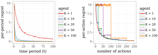
### Visual Description
## Chart Type: Comparative Line Graphs
### Overview
The image presents two line graphs comparing the performance of different agents (K=1, K=10, K=20, K=50, K=100) based on regret. The left graph shows "per-period regret" over "time period (t)", while the right graph shows "per-action regret" over "number of actions". The graphs illustrate how regret changes with time and actions for each agent.
### Components/Axes
**Left Graph:**
* **Title:** per-period regret
* **X-axis:** time period (t)
* Scale: 0 to 100, with tick marks at 0, 25, 50, 75, and 100.
* **Y-axis:** per-period regret
* Scale: 0 to 10, with tick marks at 0, 2.5, 5, 7.5, and 10.
* **Legend:** Located at the top-right of the left graph.
* K = 1 (Red)
* K = 10 (Blue)
* K = 20 (Green)
* K = 50 (Purple)
* K = 100 (Orange)
**Right Graph:**
* **Title:** per-action regret
* **X-axis:** number of actions
* Scale: 0 to 250, with tick marks at 0, 50, 100, 150, 200, and 250.
* **Y-axis:** per-action regret
* Scale: 0 to 10, with tick marks at 0, 2.5, 5, 7.5, and 10.
* **Legend:** Located at the top-right of the right graph.
* K = 1 (Red)
* K = 10 (Blue)
* K = 20 (Green)
* K = 50 (Purple)
* K = 100 (Orange)
### Detailed Analysis
**Left Graph (per-period regret vs. time period):**
* **K = 1 (Red):** Starts at approximately 10 and decreases rapidly initially, then decreases more slowly, stabilizing around a value of approximately 1 after t=50.
* **K = 10 (Blue):** Starts at approximately 10 and decreases rapidly to near 0 by t=25.
* **K = 20 (Green):** Starts at approximately 10 and decreases rapidly to near 0 by t=25.
* **K = 50 (Purple):** Starts at approximately 10 and decreases rapidly to near 0 by t=25.
* **K = 100 (Orange):** Starts at approximately 10 and decreases rapidly to near 0 by t=25.
**Right Graph (per-action regret vs. number of actions):**
* **K = 1 (Red):** Starts at approximately 10, decreases to approximately 5 around action 25, then increases again to approximately 10, and remains there.
* **K = 10 (Blue):** Starts at approximately 10, decreases to approximately 3.5 around action 40, then drops to approximately 1.5 around action 60, and remains there.
* **K = 20 (Green):** Starts at approximately 10, decreases to approximately 3.5 around action 40, then drops to approximately 1.5 around action 60, and remains there.
* **K = 50 (Purple):** Starts at approximately 10, decreases to approximately 3.5 around action 40, then drops to approximately 1.5 around action 60, and remains there.
* **K = 100 (Orange):** Starts at approximately 10, remains there until action 100, then drops to approximately 1.5 around action 120, and remains there.
### Key Observations
* In the left graph, agents K=10, K=20, K=50, and K=100 converge to a low per-period regret much faster than agent K=1.
* In the right graph, agent K=1 exhibits a different behavior, with the regret increasing after an initial decrease.
* Agents K=10, K=20, K=50, and K=100 show a stepwise decrease in per-action regret.
### Interpretation
The graphs suggest that agents with K > 1 (K=10, K=20, K=50, K=100) learn more efficiently than agent K=1, achieving lower per-period regret over time. The right graph indicates that the per-action regret for K=1 initially decreases but then increases, suggesting that this agent may be exploring suboptimal actions. The stepwise decrease in per-action regret for the other agents suggests that they are adapting their strategies in discrete stages. The agent K=100 maintains a high regret for a longer number of actions before dropping to a low regret.
</details>
- (a) per-action regret over time
- (b) per-action regret over actions
Figure 6.4: Performance of concurrent Thompson sampling.
As discussed in (Scott, 2010), concurrence plays an important role in web services, where at any time, a system may experiment by providing
different versions of a service to different users. Concurrent TS offers a natural approach for such contexts. The version discussed above involves synchronous action selection and posterior updating. In some applications, it is more appropriate to operate asynchronously, with actions selected on demand and the posterior distribution updated as data becomes available. The efficiency of synchronous and asynchronous variations of concurrent TS is studied in (Kandasamy et al. , 2018). There are also situations where an agent can alter an action based on recent experience of other agents, within a period before the action is complete. For example, in the online shortest path problem, an agent may decide to change course to avoid an edge if new observations made by other agents indicate a long expected travel time. Producing a version of TS that effectively adapts to such information while still exploring in a reliably efficient manner requires careful design, as explained in (Dimakopoulou and Van Roy, 2018).
## Further Examples
As contexts for illustrating the workings of TS, we have presented the Bernoulli bandit and variations of the online shortest path problem. To more broadly illustrate the scope of TS and issues that arise in various kinds of applications, we present several additional examples in this section.
## 7.1 News Article Recommendation
Let us start with an online news article recommendation problem in which a website needs to learn to recommend personalized and contextsensitive news articles to its users, as has been discussed in (Li et al. , 2010) and (Chapelle and Li, 2011). The website interacts with a sequence of users, indexed by t ∈ { 1 , 2 , . . . } . In each round t , it observes a feature vector z t ∈ R d associated with the t th user, chooses a news article x t to display from among a set of k articles X = { 1 , . . . , k } , and then observes a binary reward r t ∈ { 0 , 1 } indicating whether the user liked this article.
The user's feature vector might, for example, encode the following information:
- The visiting user's recent activities, such as the news articles the user has read recently.
- The visiting user's demographic information, such as the user's gender and age.
- The visiting user's contextual information, such as the user's location and the day of week.
Interested readers can refer to Section 5.2.2 of (Li et al. , 2010) for an example of feature construction in a practical context.
Following section 5 of (Chapelle and Li, 2011), we model the probability a user with features z t likes a given article x t through a logit model. Specifically, each article x ∈ X is associated with a d -dimensional parameter vector θ x ∈ R d . Conditioned on x t , θ x t and z t , a positive review occurs with probability g ( z T t θ x t ), where g is the logistic function, given by g ( a ) = 1 / (1 + e -a ). The per-period regret of this problem is defined by
$$\begin{array} { r } { \, r e g r e t _ { t } \left ( \theta _ { 1 } , \dots , \theta _ { K } \right ) = \max _ { x \in \mathcal { X } } g ( z _ { t } ^ { T } \theta _ { x } ) - g ( z _ { t } ^ { T } \theta _ { x _ { t } } ) \quad \forall t = 1 , 2 , \dots } \end{array}$$
and measures the gap in quality between the recommended article x t and the best possible recommendation that could be made based on the user's features. This model allows for generalization across users, enabling the website to learn to predict whether a user with given features z t will like a news article based on experience recommending that article to different users.
As in the path recommendation problem treated in Section 5, this problem is not amenable to efficient exact Bayesian inference. Consequently, we applied two approximate Thompson sampling methods: one samples from a Laplace approximation of the posterior (see Section 5.2) and the other uses Langevin Monte Carlo to generate an approximate posterior sample (see Section 5.3). To offer a baseline, we also applied the /epsilon1 -greedy algorithm, and searched over values of /epsilon1 for the best performer.
We present simulation results for a simplified synthetic setting with K = |X| = 3 news articles and feature dimension d = 7. At each time t ∈ { 1 , 2 , · · · } , the feature vector z t has constant 1 as its first component and each of its other components is independently
drawn from a Bernoulli distribution with success probability 1 / 6. Each components of z t could, for example, indicate presence of a particular feature, like whether the user is a woman or is accessing the site from within the United States, in which the corresponding component of θ x would reflect whether users with this feature tend to enjoy article x more than other users, while the first component of θ x reflects the article's overall popularity.
Figure 7.1: Performance of different algorithms applied to the news article recommendation problem.
<details>
<summary>Image 15 Details</summary>
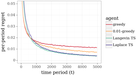
### Visual Description
## Line Chart: Per-Period Regret vs. Time Period for Different Agents
### Overview
The image is a line chart comparing the per-period regret of four different agents (greedy, 0.01-greedy, Langevin TS, and Laplace TS) over time. The x-axis represents the time period, and the y-axis represents the per-period regret. The chart shows how the regret changes for each agent as the time period increases.
### Components/Axes
* **Title:** There is no explicit title on the chart.
* **X-axis:**
* Label: "time period (t)"
* Scale: 0 to 5000, with markers at 0, 1000, 2000, 3000, 4000, and 5000.
* **Y-axis:**
* Label: "per-period regret"
* Scale: 0 to 0.05, with markers at 0, 0.01, 0.02, 0.03, 0.04, and 0.05.
* **Legend:** Located on the right side of the chart.
* greedy (red line)
* 0.01-greedy (orange line)
* Langevin TS (green line)
* Laplace TS (blue line)
### Detailed Analysis
* **Greedy (Red):** The per-period regret starts high (approximately 0.05) and decreases rapidly initially. It then plateaus around 0.013 after approximately 2000 time periods, with some fluctuations.
* At time period 0: ~0.05
* At time period 1000: ~0.018
* At time period 5000: ~0.013
* **0.01-greedy (Orange):** Similar to the greedy agent, the regret starts high (approximately 0.05) and decreases rapidly. It plateaus around 0.011 after approximately 2000 time periods, with some fluctuations.
* At time period 0: ~0.05
* At time period 1000: ~0.014
* At time period 5000: ~0.011
* **Langevin TS (Green):** The regret starts high (approximately 0.05) and decreases rapidly. It plateaus around 0.005 after approximately 2000 time periods, with some fluctuations.
* At time period 0: ~0.05
* At time period 1000: ~0.009
* At time period 5000: ~0.005
* **Laplace TS (Blue):** The regret starts high (approximately 0.05) and decreases rapidly. It plateaus around 0.005 after approximately 2000 time periods, with some fluctuations.
* At time period 0: ~0.05
* At time period 1000: ~0.008
* At time period 5000: ~0.004
### Key Observations
* All agents exhibit a rapid decrease in per-period regret during the initial time periods.
* The regret plateaus for all agents after approximately 2000 time periods.
* The Langevin TS and Laplace TS agents achieve significantly lower regret compared to the greedy and 0.01-greedy agents.
* The greedy agent has the highest final regret, followed by the 0.01-greedy agent.
### Interpretation
The chart demonstrates the performance of different reinforcement learning agents in terms of per-period regret over time. The Thompson Sampling (TS) based agents (Langevin TS and Laplace TS) outperform the greedy and 0.01-greedy agents, indicating that exploration strategies like Thompson Sampling can lead to better long-term performance. The initial rapid decrease in regret suggests that all agents quickly learn to avoid the worst actions, while the plateau indicates a convergence towards a stable policy. The difference in plateau levels highlights the effectiveness of different exploration strategies in minimizing regret.
</details>
Figure 7.1 presents results from applying Laplace and Langevin Monte Carlo approximations of Thompson sampling as well as greedy and /epsilon1 -greedy algorithms. The plots in Figure 7.1 are generated by averaging over 2 , 000 random problem instances. In each instance, the θ x 's were independently sampled from N (0 , I ), where I is the 7 × 7 identity matrix. Based on our simulations, the /epsilon1 -greedy algorithm incurred lowest regret with /epsilon1 = 0 . 01. Even with this optimized value, it is substantially outperformed by Thompson sampling.
We conclude this section by discussing some extensions to the simplified model presented above. One major limitation is that the current model does not allow for generalization across news articles. The website needs to estimate θ x separately for each article x ∈ X , and can't leverage data on the appeal of other, related, articles when doing so. Since today's news websites have thousands or even millions
of articles, this is a major limitation in practice. Thankfully, alternative models allow for generalization across news articles as well as users. One such model constructs a feature vector z t,x that encodes features of the t th user, the article x , and possibly interactions between these. Because the feature vector also depends on x , it is without loss of generality to restrict to a parameter vector θ x = θ that is common across articles. The probability user t likes the article x t is given by g ( z /latticetop t,x t θ ). Such generalization models enable us to do 'transfer learning,' i.e. to use information gained by recommending one article to reduce the uncertainty about the weight vector of another article.
Another limitation of the considered model is that the news article set X is time-invariant. In practice, the set of relevant articles will change over time as fresh articles become available or some existing articles become obsolete. Even with generalization across news articles, a time-varying news article set, or both, the considered online news article recommendation problem is still a contextual bandit problem. As discussed in Section 6.2, all the algorithms discussed in this subsection are also applicable to those cases, after some proper modifications.
## 7.2 Product Assortment
Let us start with an assortment planning problem. Consider an agent who has an ample supply of each of n different products, indexed by i = 1 , 2 , . . . , n . The seller collects a profit of p i per unit sold of product type i . In each period, the agent has the option of offering a subset of the products for sale. Products may be substitutes or complements, and therefore the demand for a product may be influenced by the other products offered for sale in the same period. In order to maximize her profit, the agent needs to carefully select the optimal set of products to offer in each period. We can represent the agent's decision variable in each period as a vector x ∈ { 0 , 1 } n where x i = 1 indicates that product i is offered and x i = 0 indicates that it is not. Upon offering an assortment containing product i in some period, the agent observes a random log-Gaussian-distributed demand d i . The mean of this log-Gaussian distribution depends on the entire assortment x and an uncertain matrix
θ ∈ R k × k . In particular
$$\log ( d _ { i } ) | \theta , x \sim N \left ( ( \theta x ) _ { i } , \sigma ^ { 2 } \right )$$
where σ 2 is a known parameter that governs the level of idiosyncratic randomness in realized demand across periods. For any product i contained in the assortment x ,
/negationslash
$$( \theta x ) _ { i } = \theta _ { i i } + \sum _ { j \neq i } x _ { j } \theta _ { i j } ,$$
where θ ii captures the demand rate for item i if it were the sole product offered and each θ ij captures the effect availability of product j has on demand for product i . When an assortment x is offered, the agent earns expected profit
$$\mathbb { E } \left [ \sum _ { i = 1 } ^ { n } p _ { i } x _ { i } d _ { i } | \theta , x \right ] = \sum _ { i = 1 } ^ { n } p _ { i } x _ { i } e ^ { ( \theta x ) _ { i } + \frac { \sigma ^ { 2 } } { 2 } } .$$
If θ were known, the agent would always select the assortment x that maximizes her expected profit in (7.1). However, when θ is unknown, the agent needs to learn to maximize profit by exploring different assortments and observing the realized demands.
TS can be adopted as a computationally efficient solution to this problem. We assume the agent begins with a multivariate Gaussian prior over θ . Due to conjugacy properties of Gaussian and log-Gaussian distributions, the posterior distribution of θ remains Gaussian after any number of periods. At the beginning of each t 'th period, the TS algorithm draws a sample ˆ θ t from this Gaussian posterior distribution. Then, the agent selects an assortment that would maximize her expected profit in period t if the sampled ˆ θ t were indeed the true parameter.
As in Examples 4.1 and 4.2, the mean and covariance matrix of the posterior distribution of θ can be updated in closed form. However, because θ is a matrix rather than a vector, the explicit form of the update is more complicated. To describe the update rule, we first introduce ¯ θ as the vectorized version of θ which is generated by stacking the columns of θ on top of each other. Let x be the assortment selected in a period, i 1 , i 2 , . . . , i k denote the the products included in this assortment (i.e.,
supp( x ) = { i 1 , i 2 , . . . , i k } ) and z ∈ R k be defined element-wise as
$$z _ { j } = \ln ( d _ { i _ { j } } ) , \, j = 1 , 2 , \dots , k .$$
Let S be a k × n 'selection matrix' where S j,i j = 1 for j = 1 , 2 , . . . , k and all its other elements are 0. Also, define
$$W = x ^ { \top } \otimes S ,$$
where ⊗ denotes the Kronecker product of matrices. At the end of current period, the posterior mean µ and covariance matrix Σ of ¯ θ are updated according to the following rules:
$$\begin{array} { r l r } { \mu } & { \leftarrow \, \left ( \Sigma ^ { - 1 } + \frac { 1 } { \sigma ^ { 2 } } W ^ { \top } W \right ) ^ { - 1 } \left ( \Sigma ^ { - 1 } \mu + \frac { 1 } { \sigma ^ { 2 } } W ^ { \top } z \right ) , } \\ & { \Sigma } & { \leftarrow \, \left ( \Sigma ^ { - 1 } + \frac { 1 } { \sigma ^ { 2 } } W ^ { \top } W \right ) ^ { - 1 } . } \end{array}$$
To investigate the performance of TS in this problem, we simulated a scenario with n = 6 and σ 2 = 0 . 04. We take the profit associated to each product i to be p i = 1 / 6. As the prior distribution, we assumed that each element of θ is independent and Gaussian-distributed with mean 0, the diagonal elements have a variance of 1, and the off-diagonal elements have a variance of 0 . 2. To understand this choice, recall the impact of diagonal and off-diagonal elements of θ . The diagonal element θ ii controls the mean demand when only product i is available, and reflects the inherent quality or popularity of that item. The off-diagonal element θ ij captures the influence availability of product j has on mean demand for product i . Our choice of prior covariance encodes that the dominant effect on demand of a product is likely its own characteristics, rather than its interaction with any single other product. Figure 7.2 presents the performance of different learning algorithms in this problem. In addition to TS, we have simulated the greedy and /epsilon1 -greedy algorithms for various values of /epsilon1 . We found that /epsilon1 = 0 . 07 provides the best performance for /epsilon1 -greedy in this problem.
As illustrated by this figure, the greedy algorithm performs poorly in this problem while /epsilon1 -greedy presents a much better performance. We found that the performance of /epsilon1 -greedy can be improved by using an annealing /epsilon1 of m m + t at each period t . Our simulations suggest using
m = 9 for the best performance in this problem. Figure 7.2 shows that TS outperforms both variations of /epsilon1 -greedy in this problem.
Figure 7.2: Regret experienced by different learning algorithms applied to product assortment problem.
<details>
<summary>Image 16 Details</summary>
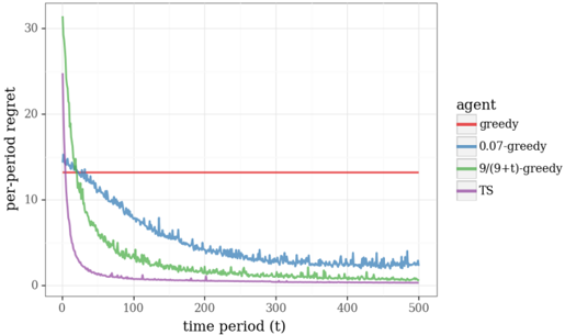
### Visual Description
## Line Chart: Per-Period Regret vs. Time Period for Different Agents
### Overview
The image is a line chart comparing the per-period regret of four different agents (greedy, 0.07-greedy, 9/(9+t)-greedy, and TS) over time. The x-axis represents the time period (t), ranging from 0 to 500. The y-axis represents the per-period regret, ranging from 0 to 30. The chart illustrates how the regret changes for each agent as the time period increases.
### Components/Axes
* **X-axis:**
* Label: "time period (t)"
* Scale: 0 to 500, with markers at 0, 100, 200, 300, 400, and 500.
* **Y-axis:**
* Label: "per-period regret"
* Scale: 0 to 30, with markers at 0, 10, 20, and 30.
* **Legend (Top-Right):**
* "agent"
* Red: "greedy"
* Blue: "0.07-greedy"
* Green: "9/(9+t)-greedy"
* Purple: "TS"
### Detailed Analysis
* **Greedy (Red):** The red line representing the "greedy" agent remains constant at a per-period regret of approximately 13.5.
* **0.07-greedy (Blue):** The blue line representing the "0.07-greedy" agent starts at a regret of approximately 15 and decreases over time, stabilizing around a regret of approximately 3 after 300 time periods.
* **9/(9+t)-greedy (Green):** The green line representing the "9/(9+t)-greedy" agent starts at a regret of approximately 31 and decreases rapidly, stabilizing around a regret of approximately 2 after 200 time periods.
* **TS (Purple):** The purple line representing the "TS" agent starts at a regret of approximately 24 and decreases rapidly, stabilizing around a regret of approximately 0.5 after 100 time periods.
### Key Observations
* The "greedy" agent has a constant regret over time.
* The "0.07-greedy", "9/(9+t)-greedy", and "TS" agents all show decreasing regret over time, with "TS" converging to a low regret value most quickly.
* The "TS" agent achieves the lowest regret value among all agents.
### Interpretation
The chart demonstrates the performance of different exploration strategies in a reinforcement learning setting, as measured by per-period regret. The "greedy" agent, which does not explore, maintains a constant regret. The other agents, which incorporate exploration, show decreasing regret as they learn the optimal policy. The "TS" agent, which uses Thompson Sampling, appears to be the most effective exploration strategy, as it converges to a low regret value most quickly. The "9/(9+t)-greedy" agent also performs well, converging to a low regret value, but not as quickly as the "TS" agent. The "0.07-greedy" agent converges slower than the "9/(9+t)-greedy" and "TS" agents.
</details>
## 7.3 Cascading Recommendations
We consider an online recommendation problem in which an agent learns to recommend a desirable list of items to a user . As a concrete example, the agent could be a search engine and the items could be web pages. We consider formulating this problem as a cascading bandit , in which user selections are governed by a cascade model , as is commonly used in the fields of information retrieval and online advertising (Craswell et al. , 2008).
A cascading bandit model is identified by a triple ( K,J,θ ), where K is the number of items, J ≤ K is the number of items recommended in each period, and θ ∈ [0 , 1] K is a vector of attraction probabilities . At the beginning of each t th period, the agent selects and presents to the user an ordered list x t ∈ { 1 , . . . , K } J . The user examines items in x t sequentially, starting from x t, 1 . Upon examining item x t,j , the user finds it attractive with probability θ x t,j . In the event that the user finds the item attractive, he selects the item and leaves the system. Otherwise, he carries on to examine the next item in the list, unless j = J , in
which case he has already considered all recommendations and leaves the system.
The agent observes y t = j if the user selects x t,j and y t = ∞ if the user does not click any item. The associated reward r t = r ( y t ) = 1 { y t ≤ J } indicates whether any item was selected. For each list x = ( x 1 , . . . , x J ) and θ ′ ∈ [0 , 1] K , let
$$\begin{array} { r } { h ( x , \theta ^ { \prime } ) = 1 - \prod _ { j = 1 } ^ { J } \left [ 1 - \theta _ { x _ { j } } ^ { \prime } \right ] . } \end{array}$$
Note that the expected reward at time t is E [ r t | x t , θ ] = h ( x t , θ ). The optimal solution x ∗ ∈ argmax x : | x | = J h ( x, θ ) consists of the J items with largest attraction probabilities. Per-period regret is given by regret t ( θ ) = h ( x ∗ , θ ) -h ( x t , θ ).
## Algorithm
CascadeUCB( K,J,α,β )
```
\frac{CascadeUCB(K, J,\alpha,\beta)}{1: for t = 1,2,... do
2:
3:
4:
5:
6:
7:
8:
9:
10:
11:
12:
13:
14:
15:
16: end for
```
## 7.1 Algorithm
CascadeTS( K,J,α,β )
```
CAScaleTS(K, J, \alpha, \beta)
1: for t = 1,2,... do
2: #sample model:
for k = 1,..., K do
Sample $\hat{k}~\text{Beta}(\alpha_{k},\beta_{k})$
5: end for
6:
7: #select and apply action:
x_t <- argmaxx:|x|=J h(x, \hat{\theta})
8:
9: Apply $x_t$ and observe $y_t$ and $r_t$
10:
11: #update posterior:
for j = 1,..., min{y_{t}, J} do
\alpha_{x_t,j} <- \alpha_{x_t,j} + 1(j = y_t)
\beta_{x_t,j} <- \beta_{x_t,j} + 1(j < y_t)
14: end for
```
Kveton et al. (2015) proposed learning algorithms for cascading bandits based on itemwise upper confidence bound (UCB) estimates. CascadeUCB (Algorithm 7.1) is a practical variant that allows for specification of prior parameters ( α, β ) that guide the early behavior of the algorithm. CascadeUCB computes a UCB U t ( k ) for each item k ∈ { 1 , . . . , K } and then chooses a list that maximizes h ( · , U t ), which represents an upper confidence bound on the list attraction probability. The list x t can be efficiently generated by choosing the J items
7.2
with highest UCBs. Upon observing the user's response, the algorithm updates the sufficient statistics ( α, β ), which count clicks and views for all the examined items. CascadeTS (Algorithm 7.2) is a Thompson sampling algorithm for cascading bandits. CascadeTS operates in a manner similar to CascadeUCB except that x t is computed based on the sampled attraction probabilities ˆ θ , rather than the itemwise UCBs U t .
In this section, we consider a specific form of UCB, which is defined by
$$U _ { t } ( k ) = \frac { \alpha _ { k } } { \alpha _ { k } + \beta _ { k } } + c \sqrt { \frac { 1 . 5 \log ( t ) } { \alpha _ { k } + \beta _ { k } } } ,$$
for k ∈ { 1 , . . . , K } , where α k / ( α k + β k ) represents the expected value of the attraction probability θ k , while the second term represents an optimistic boost that encourages exploration. Notice that the parameter c ≥ 0 controls the degree of optimism . When c = 1, the above-defined UCB reduces to the standard UCB1, which is considered and analyzed in the context of cascading bandits in (Kveton et al. , 2015). In practice, we can select c through simulations to optimize performance.
Figure 7.3 presents results from applying CascadeTS and CascadeUCB based on UCB1. These results are generated by randomly sampling 1000 cascading bandit instances, K = 1000 and J = 100, in each case sampling each attraction probability θ k independently from Beta(1 , 40). For each instance, CascadeUCB and CascadeTS are applied over 20000 time periods, initialized with ( α k , β k ) = (1 , 40). The plots are of per-period regrets averaged over the 1000 simulations.
The results demonstrate that TS far outperforms this version of CascadeUCB. Why? An obvious reason is that h ( x, U t ) is far too optimistic. In particular, h ( x, U t ) represents the probability of a click if every item in x simultaneously takes on the largest attraction probability that is statistically plausible. However, due to the statistical independence of item attractions, the agent is unlikely to have substantially under-estimated the attraction probability of every item in x . As such, h ( x, U t ) tends to be far too optimistic. CascadeTS, on the other hand, samples components ˆ θ k independently across items. While any sample ˆ θ k might deviate substantially from its mean, it is unlikely that the
Figure 7.3: Comparison of CascadeTS and CascadeUCB with K = 1000 items and J = 100 recommendations per period.
<details>
<summary>Image 17 Details</summary>
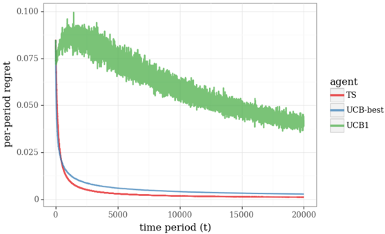
### Visual Description
## Chart: Per-Period Regret vs. Time Period for Different Agents
### Overview
The image is a line chart comparing the per-period regret of three different agents (TS, UCB-best, and UCB1) over a time period of 20,000 units. The chart displays how the regret changes over time for each agent.
### Components/Axes
* **X-axis:** "time period (t)". Scale ranges from 0 to 20000, with tick marks at 0, 5000, 10000, 15000, and 20000.
* **Y-axis:** "per-period regret". Scale ranges from 0 to 0.100, with tick marks at 0, 0.025, 0.050, 0.075, and 0.100.
* **Legend (located on the right side of the chart):**
* Red line: TS (Thompson Sampling)
* Blue line: UCB-best (Upper Confidence Bound - best)
* Green line: UCB1 (Upper Confidence Bound 1)
### Detailed Analysis
* **TS (Red Line):** The per-period regret starts at approximately 0.075 and rapidly decreases to approximately 0.002 by time period 5000. It then remains relatively constant at around 0.002 for the rest of the time period.
* **UCB-best (Blue Line):** The per-period regret starts at approximately 0.075 and decreases to approximately 0.005 by time period 5000. It then remains relatively constant at around 0.005 for the rest of the time period.
* **UCB1 (Green Line):** The per-period regret starts at approximately 0.075, increases to approximately 0.095 around time period 2500, and then gradually decreases to approximately 0.040 by time period 20000. The line exhibits significant fluctuations throughout the entire time period.
### Key Observations
* TS and UCB-best perform significantly better than UCB1 in terms of per-period regret.
* TS has the lowest per-period regret after the initial time period.
* UCB1 has a higher initial regret and exhibits more fluctuation than the other two agents.
### Interpretation
The chart demonstrates the performance of three different reinforcement learning agents in terms of per-period regret over time. The results suggest that Thompson Sampling (TS) and UCB-best are more effective at minimizing regret compared to UCB1 in this particular scenario. The initial exploration phase seems to have a higher regret for all agents, but TS and UCB-best quickly converge to a low regret value, while UCB1's regret remains significantly higher and more volatile. This could be due to the exploration-exploitation trade-off handled differently by each algorithm. TS and UCB-best likely exploit better actions more quickly, while UCB1 might continue to explore less promising actions for a longer period.
</details>
sampled attraction probability of every item in x greatly exceeds its mean. As such, the variability in h ( x, ˆ θ ) provides a much more accurate reflection of the magnitude of uncertainty.
The plot labeled 'UCB-best' in Figure 7.3 illustrates performance of CascadeUCB with c = 0 . 05, which approximately minimizes cumulative regret over 20,000 time periods. It is interesting that even after being tuned to the specific problem and horizon, the performance of CascadeUCB falls short of Cascade TS. A likely source of loss stems from the shape of confidence sets used by CascadeUCB. Note that the algorithm uses hyper-rectangular confidence sets, since the set of statistically plausible attraction probability vectors is characterized by a Cartesian product item-level confidence intervals. However, the Bayesian central limit theorem suggests that 'ellipsoidal" confidence sets offer a more suitable choice. Specifically, as data is gathered, the posterior distribution over θ can be well approximated by a multivariate Gaussian, for which level sets are ellipsoidal. Losses due to the use of hyper-rectangular confidence sets have been studied through regret analysis in (Dani et al. , 2008) and through simple analytic examples in (Osband and Van Roy, 2017a).
It is worth noting that tuned versions of CascadeUCB do sometimes perform as well or better than CascadeTS. Figure 7.4 illustrates an example of this. The setting is identical to that used to generate the results of Figure 7.3, except that K = 50 and J = 10, and cumulative regret is approximately optimized with c = 0 . 1. CascadeUCB with the optimally tuned c outperforms CascadeTS. This qualitative difference from the case of K = 1000 and J = 100 is likely due to the fact that hyper-rectangular sets offer poorer approximations of ellipsoids as the dimension increases. This phenomenon and its impact on regret aligns with theoretical results of (Dani et al. , 2008). That said, CascadeUCB is somewhat advantaged in this comparison because it is tuned specifically for the setting and time horizon.
Figure 7.4: Comparison of CascadeTS and CascadeUCB with K = 50 items and J = 10 recommendations per period.
<details>
<summary>Image 18 Details</summary>
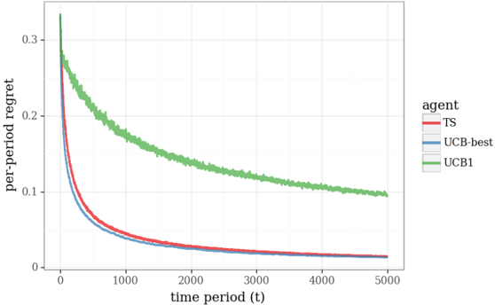
### Visual Description
## Line Chart: Per-Period Regret vs. Time Period for Different Agents
### Overview
The image is a line chart comparing the per-period regret of three different agents (TS, UCB-best, and UCB1) over a time period ranging from 0 to 5000. The chart displays how the regret changes over time for each agent.
### Components/Axes
* **X-axis:** "time period (t)" with a scale from 0 to 5000, incrementing by 1000.
* **Y-axis:** "per-period regret" with a scale from 0 to 0.3, incrementing by 0.1.
* **Legend (top-right):**
* Red line: TS (Thompson Sampling)
* Blue line: UCB-best (Upper Confidence Bound - best)
* Green line: UCB1 (Upper Confidence Bound 1)
### Detailed Analysis
* **TS (Red):** The red line represents the Thompson Sampling agent. It starts at approximately 0.28 regret and rapidly decreases, stabilizing around 0.02 after approximately 2000 time periods.
* **UCB-best (Blue):** The blue line represents the UCB-best agent. It starts at approximately 0.25 regret and also rapidly decreases, closely following the TS agent and stabilizing around 0.02 after approximately 2000 time periods.
* **UCB1 (Green):** The green line represents the UCB1 agent. It starts at approximately 0.32 regret and decreases at a slower rate compared to TS and UCB-best. It stabilizes around 0.10 after approximately 4000 time periods.
### Key Observations
* Both TS and UCB-best agents exhibit significantly lower regret compared to the UCB1 agent, especially after 2000 time periods.
* The regret for TS and UCB-best converges to a similar low value.
* UCB1's regret decreases more slowly and stabilizes at a higher value than the other two agents.
### Interpretation
The chart demonstrates that Thompson Sampling (TS) and UCB-best algorithms perform significantly better in terms of minimizing per-period regret compared to the UCB1 algorithm in this scenario. The rapid decrease in regret for TS and UCB-best suggests faster learning and adaptation to the environment. The higher and slower-decreasing regret of UCB1 indicates a less efficient exploration-exploitation strategy in this context. The convergence of TS and UCB-best suggests that, given enough time, they achieve similar levels of performance. The data suggests that for this specific problem, TS and UCB-best are more effective algorithms for minimizing regret over time.
</details>
## 7.4 Active Learning with Neural Networks
Neural networks are widely used in supervised learning, where given an existing set of predictor-response data pairs, the objective is to produce a model that generalizes to accurately predict future responses conditioned on associated predictors. They are also increasingly being used to guide actions ranging from recommendations to robotic maneuvers. Active
learning is called for to close the loop by generating actions that do not solely maximize immediate performance but also probe the environment to generate data that accelerates learning. TS offers a useful principle upon which such active learning algorithms can be developed.
With neural networks or other complex model classes, computing the posterior distribution over models becomes intractable. Approximations are called for, and incremental updating is essential because fitting a neural network is a computationally intensive task in its own right. In such contexts, ensemble sampling offers a viable approach (Lu and Van Roy, 2017). In Section 5.6, we introduced a particular mechanism for ensemble sampling based on the bootstrap. In this section, we consider an alternative version of ensemble sampling and present results from (Lu and Van Roy, 2017) that demonstrate its application to active learning with neural networks.
To motivate our algorithm, let us begin by discussing how it can be applied to the linear bandit problem.
Example 7.1. (Linear Bandit) Let θ be drawn from R M and distributed according to a N ( µ 0 , Σ 0 ) prior. There is a set of K actions X ⊆ R M . At each time t = 1 , . . . , T , an action x t ∈ X is selected, after which a reward r t = y t = θ /latticetop x t + w t is observed, where w t ∼ N (0 , σ 2 w ).
In this context, ensemble sampling is unwarranted, since exact Bayesian inference can be carried out efficiently via Kalman filtering. Nevertheless, the linear bandit offers a simple setting for explaining the workings of an ensemble sampling algorithm.
Consider maintaining a covariance matrix updated according to
$$\Sigma _ { t + 1 } = \left ( \Sigma _ { t } ^ { - 1 } + x _ { t } x _ { t } ^ { \top } / \sigma _ { w } ^ { 2 } \right ) ^ { - 1 } ,$$
and N models θ 1 t , . . . , θ N t , initialized with θ 1 1 , . . . , θ N 1 each drawn independently from N ( µ 0 , Σ 0 ) and updated incrementally according to
$$\overline { \theta } _ { t + 1 } ^ { n } = \Sigma _ { t + 1 } \left ( \Sigma _ { t } ^ { - 1 } \overline { \theta } _ { t } ^ { n } + x _ { t } ( y _ { t } + \tilde { w } _ { t } ^ { n } ) / \sigma _ { w } ^ { 2 } \right ) ,$$
for n = 1 , . . . , N , where ( ˜ w n t : t = 1 , . . . , T, n = 1 , . . . , N ) are independent N (0 , σ 2 w ) random samples drawn by the updating algorithm. It is
easy to show that the resulting parameter vectors satisfy
$$\overline { \theta } _ { t } ^ { n } = \arg \min _ { \nu } \left ( \frac { 1 } { \sigma _ { w } ^ { 2 } } \sum _ { \tau = 1 } ^ { t - 1 } ( y _ { \tau } + \tilde { w } _ { \tau } ^ { n } - x _ { \tau } ^ { \top } \nu ) ^ { 2 } + ( \nu - \overline { \theta } _ { 1 } ^ { n } ) ^ { \top } \Sigma _ { 0 } ^ { - 1 } ( \nu - \overline { \theta } _ { 1 } ^ { n } ) \right ) .$$
Thich admits an intuitive interpretation: each θ n t is a model fit to a randomly perturbed prior and randomly perturbed observations. As established in (Lu and Van Roy, 2017), for any deterministic sequence x 1 , . . . , x t -1 , conditioned on the history, the models θ 1 t , . . . , θ N t are independent and identically distributed according to the posterior distribution of θ . In this sense, the ensemble approximates the posterior.
The ensemble sampling algorithm we have described for the linear bandit problem motivates an analogous approach for the following neural network model.
Example 7.2. (Neural Network) Let g θ : R M ↦→ R K denote a mapping induced by a neural network with weights θ . Suppose there are K actions X ⊆ R M , which serve as inputs to the neural network, and the goal is to select inputs that yield desirable outputs. At each time t = 1 , . . . , T , an action x t ∈ X is selected, after which y t = g θ ( x t ) + w t is observed, where w t ∼ N (0 , σ 2 w I ). A reward r t = r ( y t ) is associated with each observation. Let θ be distributed according to a N ( µ 0 , Σ 0 ) prior. The idea here is that data pairs ( x t , y t ) can be used to fit a neural network model, while actions are selected to trade off between generating data pairs that reduce uncertainty in neural network weights and those that offer desirable immediate outcomes.
Consider an ensemble sampling algorithm that once again begins with N independent models with connection weights θ 1 1 , . . . , θ N 1 sampled from a N ( µ 0 , Σ 0 ) prior. It could be natural here to let µ 0 = 0 and Σ 0 = σ 2 0 I for some variance σ 2 0 chosen so that the range of probable models spans plausible outcomes. To incrementally update parameters, at each time t , each n th model applies some number of stochastic gradient descent iterations to reduce a loss function of the form
$$\mathcal { L } _ { t } ( \nu ) = \frac { 1 } { \sigma _ { w } ^ { 2 } } \sum _ { \tau = 1 } ^ { t - 1 } ( y _ { \tau } + \tilde { w } _ { \tau } ^ { n } - g _ { \nu } ( x _ { \tau } ) ) ^ { 2 } + ( \nu - \overline { \theta } _ { 1 } ^ { n } ) ^ { \top } \Sigma _ { 0 } ^ { - 1 } ( \nu - \overline { \theta } _ { 1 } ^ { n } ) .$$
Figure 7.5 present results from simulations involving a two-layer neural network, with a set of K actions, X ⊆ R M . The weights of the neural network, which we denote by w 1 ∈ R D × N and w 2 ∈ R D , are each drawn from N (0 , λ ). Let θ ≡ ( w 1 , w 2 ). The mean reward of an action x ∈ X is given by g θ ( x ) = w /latticetop 2 max(0 , w 1 a ). At each time step, we select an action x t ∈ X and observe reward y t = g θ ( x t ) + z t , where z t ∼ N (0 , σ 2 z ). We used M = 100 for the input dimension, D = 50 for the dimension of the hidden layer, number of actions K = 100, prior variance λ = 1, and noise variance σ 2 z = 100. Each component of each action vector is sampled uniformly from [ -1 , 1], except for the last component, which is set to 1 to model a constant offset. All results are averaged over 100 realizations.
In our application of the ensemble sampling algorithm we have described, to facilitate gradient flow, we use leaky rectified linear units of the form max(0 . 01 x, x ) during training, though the target neural network is made up of regular rectified linear units as indicated above. In our simulations, each update was carried out with 5 stochastic gradient steps, with a learning rate of 10 -3 and a minibatch size of 64.
Figure 7.5: Bandit learning with an underlying neural network.
<details>
<summary>Image 19 Details</summary>
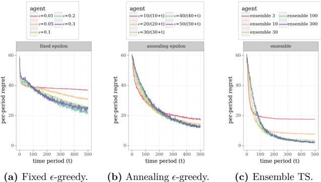
### Visual Description
## Chart Type: Multiple Line Graphs Comparing Regret over Time
### Overview
The image presents three line graphs comparing the per-period regret of different agents over time. Each graph represents a different exploration strategy: fixed epsilon-greedy, annealing epsilon-greedy, and ensemble Thompson Sampling (TS). The x-axis represents the time period (t), ranging from 0 to 500, and the y-axis represents the per-period regret, ranging from 0 to 60. Each graph plots multiple agents with different parameter settings for their respective exploration strategies.
### Components/Axes
* **X-axis (all graphs):** time period (t), scale from 0 to 500 in increments of 100.
* **Y-axis (all graphs):** per-period regret, scale from 0 to 60 in increments of 20.
* **Graph Titles:**
* (a) Fixed ε-greedy.
* (b) Annealing ε-greedy.
* (c) Ensemble TS.
* **Legends (top-left of each graph):** Each legend identifies the agent type and its corresponding parameter settings.
* **Fixed ε-greedy:**
* Red: ε = 0.01
* Orange: ε = 0.05
* Green: ε = 0.1
* Light Blue: ε = 0.2
* Dark Blue: ε = 0.3
* **Annealing ε-greedy:**
* Red: ε = 10/(10+t)
* Orange: ε = 20/(20+t)
* Green: ε = 30/(30+t)
* Light Blue: ε = 40/(40+t)
* Dark Blue: ε = 50/(50+t)
* **Ensemble TS:**
* Red: ensemble 3
* Orange: ensemble 10
* Green: ensemble 30
* Light Blue: ensemble 100
* Dark Blue: ensemble 300
### Detailed Analysis
#### (a) Fixed ε-greedy
* **Trend:** The per-period regret generally decreases initially and then plateaus. The level at which it plateaus depends on the epsilon value.
* **Data Points:**
* ε = 0.01 (Red): Starts around 60, decreases to approximately 38, and remains relatively constant.
* ε = 0.05 (Orange): Starts around 60, decreases to approximately 32, and remains relatively constant.
* ε = 0.1 (Green): Starts around 60, decreases to approximately 25, and remains relatively constant.
* ε = 0.2 (Light Blue): Starts around 60, decreases to approximately 23, and remains relatively constant.
* ε = 0.3 (Dark Blue): Starts around 60, decreases to approximately 22, and remains relatively constant.
#### (b) Annealing ε-greedy
* **Trend:** The per-period regret decreases over time for all agents.
* **Data Points:**
* ε = 10/(10+t) (Red): Starts around 60, decreases to approximately 15.
* ε = 20/(20+t) (Orange): Starts around 60, decreases to approximately 13.
* ε = 30/(30+t) (Green): Starts around 60, decreases to approximately 12.
* ε = 40/(40+t) (Light Blue): Starts around 60, decreases to approximately 11.
* ε = 50/(50+t) (Dark Blue): Starts around 60, decreases to approximately 10.
#### (c) Ensemble TS
* **Trend:** The per-period regret decreases over time, with the ensemble size affecting the rate and final regret level.
* **Data Points:**
* Ensemble 3 (Red): Starts around 60, decreases to approximately 18, and remains relatively constant.
* Ensemble 10 (Orange): Starts around 60, decreases to approximately 15, and remains relatively constant.
* Ensemble 30 (Green): Starts around 60, decreases to approximately 12, and remains relatively constant.
* Ensemble 100 (Light Blue): Starts around 60, decreases to approximately 10, and remains relatively constant.
* Ensemble 300 (Dark Blue): Starts around 60, decreases to approximately 9, and remains relatively constant.
### Key Observations
* In the fixed epsilon-greedy strategy, higher epsilon values lead to lower final regret levels but potentially slower initial learning.
* The annealing epsilon-greedy strategy consistently reduces regret over time, regardless of the initial epsilon parameter.
* In the ensemble TS strategy, larger ensemble sizes result in lower final regret levels.
### Interpretation
The graphs demonstrate the impact of different exploration strategies on per-period regret. The fixed epsilon-greedy method balances exploration and exploitation, with the epsilon value controlling this balance. The annealing epsilon-greedy method dynamically adjusts the exploration rate, leading to continuous improvement. The ensemble TS method leverages multiple models to make decisions, with larger ensembles generally performing better. The data suggests that for this particular problem, annealing epsilon-greedy and ensemble TS are more effective at minimizing regret over time compared to fixed epsilon-greedy. The ensemble TS method with larger ensemble sizes appears to be the most effective strategy.
</details>
Figure 7.5 illustrates the performance of several learning algorithms with an underlying neural network. Figure 7.5a demonstrates the per-
formance of an /epsilon1 -greedy strategy across various levels of /epsilon1 . We find that we are able to improve performance with an annealing schedule /epsilon1 = k k + t (Figure 7.5b). However, we find that an ensemble sampling strategy outperforms even the best tuned /epsilon1 -schedules (Figure 7.5c). Further, we see that ensemble sampling strategy can perform well with remarkably few members of this ensemble. Ensemble sampling with fewer members leads to a greedier strategy, which can perform better for shorter horizons, but is prone to premature and suboptimal convergence compared to true TS (Lu and Van Roy, 2017). In this problem, using an ensemble of as few as 30 members provides very good performance.
## 7.5 Reinforcement Learning in Markov Decision Processes
Reinforcement learning (RL) extends upon contextual online decision problems to allow for delayed feedback and long term consequences (Sutton and Barto, 1998; Littman, 2015). Concretely (using the notation of Section 6.2) the response y t to the action x t depends on a context z t ; but we no longer assume that the evolution of the context z t +1 is independent of y t . As such, the action x t may affect not only the reward r ( y t ) but also, through the effect upon the context z t +1 the rewards of future periods ( r ( y t ′ )) t ′ >t . As a motivating example, consider a problem of sequential product recommendations x t where the customer response y t is influenced not only by the quality of the product, but also the history of past recommendations. The evolution of the context z t +1 is then directly affected by the customer response y t ; if a customer watched 'The Godfather' and loved it, then chances are probably higher they may enjoy 'The Godfather 2.'
Maximizing cumulative rewards in a problem with long term consequences can require planning with regards to future rewards, rather than optimizing each period myopically. Similarly, efficient exploration in these domains can require balancing not only the information gained over a single period; but also the potential for future informative actions over subsequent periods. This sophisticated form of temporally-extended exploration, which can be absolutely critical for effective performance, is sometimes called deep exploration (Osband et al. , 2017). TS can be applied successfully to reinforcement learning (Osband et al. , 2013).
However, as we will discuss, special care must be taken with respect to the notion of a time period within TS to preserve deep exploration.
Consider a finite horizon Markov decision process (MDP) M = ( S , A , R M , P M , H, ρ ), where S is the state space, A is the action space, and H is the horizon. The agent begins in a state s 0 , sampled from ρ , and over each timestep h = 0 , .., H -1 the agent selects action a h ∈ A , receives a reward r h ∼ R s M h ,a h , and transitions to a new state s h +1 ∼ P s M h ,a h . Here, R s M h ,a h and P s M h ,a h are probability distributions. A policy µ is a function mapping each state s ∈ S and timestep h = 0 , .., H -1 to an action a ∈ A . The value function V M µ,h ( s ) = E [ ∑ H -1 j = h r j ( s j , µ ( s j , j )) | s h = s ] encodes the expected reward accumulated under µ over the remainder of the episode when starting from state s and timestep h . Finite horizon MDPs model delayed consequences of actions through the evolution of the state, but the scope of this influence is limited to within an individual episode.
Let us consider an episodic RL problem, in which an agent learns about R M and P M over episodes of interaction with an MDP. In each episode, the agent begins in a random state, sampled from ρ , and follows a trajectory, selecting actions and observing rewards and transitions over H timesteps. Immediately we should note that we have already studied a finite horizon MDP under different terminology in Example 1.2: the online shortest path problem. To see the connection, simply view each vertex as a state and the choice of edge as an action within a timestep. With this connection in mind we can express the problem of maximizing the cumulative rewards ∑ K k =1 ∑ H -1 h =0 r ( s kh , a kh ) in a finite horizon MDP equivalently as an online decision problem over periods k = 1 , 2 , .., K , each involving the selection of a policy µ k for use over an episode of interaction between the agent and the MDP. By contrast, a naive application of TS to reinforcement learning that samples a new policy for each timestep within an episode could be extremely inefficient as it does not perform deep exploration.
Consider the example in Figure 7.6 where the underlying MDP is characterized by a long chain of states { s -N , .., s N } and only the one of the far left or far right positions are rewarding with equal probability; all other states produce zero reward and with known dynamics. Learning about the true dynamics of the MDP requires a consistent policy over
Figure 7.6: MDPs where TS with sampling at every timestep within an episode leads to inefficient exploration.
<details>
<summary>Image 20 Details</summary>
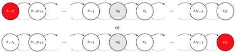
### Visual Description
## State Transition Diagram: Two Possible State Configurations
### Overview
The image presents two possible configurations of a state transition diagram. Each configuration depicts a series of states labeled from s_-N to s_N, represented as circles. The states are connected by arrows indicating possible transitions between adjacent states. The diagram illustrates two scenarios: one where the initial state s_-N is highlighted in red, and another where the final state s_N is highlighted in red. The state s_0 is highlighted in gray in both configurations.
### Components/Axes
* **States:** Represented by circles, labeled as s_-N, s_-N+1, ..., s_-1, s_0, s_1, ..., s_N-1, s_N.
* **Transitions:** Represented by curved arrows connecting adjacent states. There are two arrows between each state, one going to the left and one going to the right. The arrows going to the left are solid black, and the arrows going to the right are light gray.
* **Highlighted States:**
* Red: Indicates the initial or final state in each configuration.
* Gray: Indicates the central state s_0 in both configurations.
* **Text:** The word "or" separates the two configurations.
### Detailed Analysis or ### Content Details
**Top Configuration:**
* **Initial State:** s_-N is highlighted in red.
* **States:** The states are arranged linearly from left to right: s_-N, s_-N+1, ..., s_-1, s_0, s_1, ..., s_N-1, s_N.
* **Transitions:** Each state has a transition to its adjacent states.
* **Central State:** s_0 is highlighted in gray.
**Bottom Configuration:**
* **Final State:** s_N is highlighted in red.
* **States:** The states are arranged linearly from left to right: s_-N, s_-N+1, ..., s_-1, s_0, s_1, ..., s_N-1, s_N.
* **Transitions:** Each state has a transition to its adjacent states.
* **Central State:** s_0 is highlighted in gray.
### Key Observations
* The diagram illustrates two possible states of a system, where either the initial state (s_-N) or the final state (s_N) is active (highlighted in red).
* The central state (s_0) is consistently highlighted in gray in both configurations.
* The transitions between states are bidirectional, allowing movement between adjacent states.
### Interpretation
The diagram represents a system that can exist in a range of states, from s_-N to s_N. The two configurations suggest two possible scenarios: one where the system starts in state s_-N and progresses through the states, and another where the system ends in state s_N. The highlighting of s_0 in both configurations might indicate a central or equilibrium state. The bidirectional transitions suggest that the system can move back and forth between adjacent states. This type of diagram is commonly used to model Markov chains or other state-based systems.
</details>
N steps right or N steps left; a variant of TS that resamples after each step would be exponentially unlikely to make it to either end within N steps (Osband et al. , 2017). By contrast, sampling only once prior to each episode and holding the policy fixed for the duration of the episode demonstrates deep exploration and results in learning the optimal policy within a single episode.
In order to apply TS to policy selection we need a way of sampling from the posterior distribution for the optimal policy. One efficient way to do this, at least with tractable state and action spaces, is to maintain a posterior distribution over the rewards R M and the transition dynamics P M at each state-action pair ( s, a ). In order to generate a sample for the optimal policy, simply take a single posterior sample for the reward and transitions and then solve for the optimal policy for this sample . This is equivalent sampling from the posterior distribution of the optimal policy, but may be computationally more efficient than maintaining that posterior distribution explicitly. Estimating a posterior distribution over rewards is no different from the setting of bandit learning that we have already discussed at length within this paper. The transition function looks a little different, but for transitions over a finite state space the Dirichlet distribution is a useful conjugate prior. It is a multidimensional generalization of the Beta distribution from Example 3.1. The Dirichlet prior over outcomes in S = { 1 , .., S } is specified by a positive vector of pseudo-observations α ∈ R S + ; updates to the Dirichlet posterior can be performed simply by incrementing the appropriate column of α (Strens, 2000).
In Figure 7.7 we present a computational comparison of TS with sampling per timestep versus per episode, applied to the example of Figure 7.6. Figure 7.7a compares the performance of sampling schemes where the agent has an informative prior that matches the true un-
derlying system. As explained above, sampling once per episode TS is guaranteed to learn the true MDP structure in a single episode. By contrast, sampling per timestep leads to uniformly random actions until either s -N or s N is visited. Therefore, it takes a minimum of 2 N episodes for the first expected reward.
Figure 7.7: TS with sampling per timestep versus per episode.
<details>
<summary>Image 21 Details</summary>
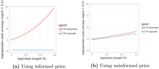
### Visual Description
## Chart: Comparison of TS timestep and TS episode agents with informed and uninformed priors
### Overview
The image presents two line charts comparing the performance of two agents, "TS timestep" and "TS episode," under different conditions: using an informed prior (left chart) and using an uninformed prior (right chart). The y-axis represents the logarithm of episodes until the average regret is less than 0.5, while the x-axis represents the logarithm of the chain length N.
### Components/Axes
* **Title (Left Chart):** (a) Using informed prior.
* **Title (Right Chart):** (b) Using uninformed prior.
* **Y-axis Label (Both Charts):** log(episodes until average regret < 0.5)
* Scale: 0 to 12, with tick marks at 0, 3, 6, 9, and 12.
* **X-axis Label (Both Charts):** log(chain length N)
* Scale: 1 to 1.6, with tick marks at 1, 1.2, 1.4, and 1.6.
* **Legend (Both Charts, Top Right):**
* TS timestep (Red line)
* TS episode (Blue line)
### Detailed Analysis
**Left Chart (Informed Prior):**
* **TS timestep (Red):** The line starts at approximately y=3 when x=1 and increases exponentially to approximately y=11.5 when x=1.6.
* **TS episode (Blue):** The line remains relatively flat, staying close to y=0.2 across the entire x-axis range (x=1 to x=1.6).
**Right Chart (Uninformed Prior):**
* **TS timestep (Red):** The line starts at approximately y=3 when x=1 and increases gradually to approximately y=5.5 when x=1.6.
* **TS episode (Blue):** The line starts at approximately y=3 when x=1 and increases gradually to approximately y=5 when x=1.6.
### Key Observations
* With an informed prior, the "TS timestep" agent requires significantly more episodes to achieve an average regret less than 0.5 as the chain length increases, while the "TS episode" agent's performance remains relatively constant.
* With an uninformed prior, both agents show a gradual increase in the number of episodes required as the chain length increases, with the "TS timestep" agent performing slightly worse than the "TS episode" agent.
* The difference in performance between the two agents is much more pronounced with an informed prior than with an uninformed prior.
### Interpretation
The data suggests that the choice of prior significantly impacts the performance of the "TS timestep" agent, particularly as the chain length increases. When an informed prior is used, the "TS timestep" agent struggles to maintain a low average regret, requiring a rapidly increasing number of episodes. In contrast, the "TS episode" agent's performance is relatively unaffected by the chain length when using an informed prior.
When an uninformed prior is used, both agents exhibit a more gradual increase in the number of episodes required as the chain length increases, suggesting that the prior knowledge plays a crucial role in the "TS timestep" agent's performance. The "TS timestep" agent performs slightly worse than the "TS episode" agent, indicating that the timestep approach may be less efficient in the absence of prior knowledge.
The charts highlight the importance of selecting an appropriate prior for the "TS timestep" agent, as an informed prior can lead to significantly worse performance compared to an uninformed prior or the "TS episode" agent. This could be due to the informed prior being misaligned with the true underlying distribution, causing the "TS timestep" agent to explore suboptimal actions.
</details>
The difference in performance demonstrated by Figure 7.7a is particularly extreme because the prior structure means that there is only value to deep exploration, and none to 'shallow' exploration (Osband et al. , 2017). In Figure 7.7b we present results for TS on the same environment but with a uniform Dirichlet prior over transitions and a standard Gaussian prior over rewards for each state-action pair. With this prior structure sampling per timestep is not as hopeless, but still performs worse than sampling per episode. Once again, this difference increases with MDP problem size. Overall, Figure 7.7 demonstrates that the benefit of sampling per episode, rather than per timestep, can become arbitrarily large. As an additional benefit this approach is also more computationally efficient, since we only need to solve for the optimal policy once every episode rather than at each timestep.
This more nuanced application of TS to RL is sometimes referred to as posterior sampling for reinforcement learning (PSRL) (Strens, 2000). Recent work has developed a theoretical analyses of PSRL that guarantee strong expected performance over a wide range of environ-
ments (Osband et al. , 2013; Osband and Van Roy, 2014b; Osband and Van Roy, 2014a; Osband and Van Roy, 2017b; Ouyang et al. , 2017). This work builds on and extends theoretical results that will be discussed in Section 8.1.2. It is worth mentioning that PSRL fits in the broader family of Bayesian approaches to efficient reinforcement learning; we refer interested readers to the survey paper (Ghavamzadeh et al. , 2015).
## Why it Works, When it Fails, and Alternative Approaches
Earlier sections demonstrate that TS approaches can be adapted to address a number of problem classes of practical import. In this section, we provide intuition for why TS explores efficiently, and briefly review theoretical work that formalizes this intuition. We will then highlight problem classes for which TS is poorly suited, and refer to some alternative algorithms.
## 8.1 Why Thompson Sampling Works
To understand whether TS is well suited to a particular application, it is useful to develop a high level understanding of why it works. As information is gathered, beliefs about action rewards are carefully tracked. By sampling actions according to the posterior probability that they are optimal, the algorithm continues to sample all actions that could plausibly be optimal, while shifting sampling away from those that are unlikely to be optimal. Roughly speaking, the algorithm tries all promising actions while gradually discarding those that are believed to underperform.This intuition is formalized in recent theoretical analyses of Thompson sampling, which we now review.
## 8.1.1 Regret Analysis for Classical Bandit Problems
Asymptotic Instance Dependent Regret Bounds. Consider the classical beta-Bernoulli bandit problem of Example 1.1. For this problem, sharp results on the asymptotic scaling of regret are available. The cumulative regret of an algorithm over T periods is
$$R e g r e t ( T ) = \sum _ { t = 1 } ^ { T } \left ( \max _ { 1 \leq k \leq K } \theta _ { k } - \theta _ { x _ { t } } \right ) ,$$
where K is the number of actions, x t ∈ { 1 , . . . , K } is the action selected at time t , and θ = ( θ 1 , . . . , θ K ) denotes action success probabilities. For each time horizon T , E [Regret( T ) | θ ] measures the expected T -period regret on the problem instance θ . The conditional expectation integrates over the noisy realizations of rewards and the algorithm's random action selection, holding fixed the success probabilities θ = ( θ 1 , . . . , θ K ). Though this is difficult to evaluate, one can show that
/negationslash
$$\lim _ { T \rightarrow \infty } \frac { \mathbb { E } [ R e g r e t ( T ) | \theta ] } { \log ( T ) } = \sum _ { k \neq k ^ { * } } \frac { \theta _ { k ^ { * } } - \theta _ { k } } { d _ { K L } ( \theta _ { k ^ { * } } | | \theta _ { k } ) } ,$$
assuming that there is a unique optimal action k ∗ . Here, d KL ( θ || θ ′ ) = θ log ( θ θ ′ ) +(1 -θ ) log ( 1 -θ 1 -θ ′ ) is the Kullback-Leibler divergence between Bernoulli distributions. The fundamental lower bound of (Lai and Robbins, 1985) shows no algorithm can improve on the scaling in (8.1), establishing a sense in which the algorithm is asymptotically optimal. That the regret of TS exhibits this scaling was first observed empirically by (Chapelle and Li, 2011). A series of papers provided proofs that formalize this finding (Agrawal and Goyal, 2012; Agrawal and Goyal, 2013a; Kauffmann et al. , 2012).
This result has been extended to cases where reward distributions are Gaussian or, more generally, members of a canonical one-dimensional exponential family (Honda and Takemura, 2014). It has also been extended to the case of Gaussian distributions with unknown variance by (Honda and Takemura, 2014), which further establishes that this result can fail to hold for a particular improper prior distribution. Although, intuitively, the effects of the prior distribution should wash out as T →∞ , all of these results apply to specific choices of uninformative
prior distributions. Establishing asymptotic optimality of TS for broader classes of prior distributions remains an interesting open issue.
Instance-Independent Regret bounds. While the results discussed in the previous section establishes that the regret of TS is optimal in some sense, it is important to understand that this result is asymptotic. Focusing on this asymptotic scaling enables sharp results, but even for problems with long time horizons, there are substantial performance differences among algorithms known to be asymptotically optimal in the sense of (8.1). The bound essentially focuses on a regime in which the agent is highly confident of which action is best but continues to occasionally explore in order to become even more confident. In particular, the bound suggests that for sufficiently large T , regret scales like
/negationslash
$$\mathbb { E } [ R e g r e t ( T ) | \theta ] \approx \sum _ { k \neq k ^ { * } } \frac { \theta _ { k ^ { * } } - \theta _ { k } } { d _ { K L } ( \theta _ { k ^ { * } } | | \theta _ { k } ) } \log ( T ) .$$
This becomes easier to interpret if we specialize to the case in which rewards, conditioned on θ , are Gaussian with unit variance, for which d KL ( θ || θ ′ ) = ( θ -θ ′ ) 2 / 2, and therefore,
/negationslash
$$\mathbb { E } [ R e g r e t ( T ) | \theta ] \approx \sum _ { k \neq k ^ { * } } \frac { 2 } { \theta _ { k ^ { * } } - \theta _ { k } } \log ( T ) .$$
The fact that the final expression is dominated by near-optimal actions reflects that in the relevant asymptotic regime other actions can be essentially ruled out using far fewer samples.
A more subtle issue is that O (log( T )) regret bounds like those described above become vacuous for problems with nearly-optimal actions, since the right-side of 8.2 can become arbitrarily large. This issue is particularly limiting for complex structured online decision problems, where there are often a large or even infinite number of near-optimal actions.
For the Bernoulli bandit problem of Example 1.1, (Agrawal and Goyal, 2013a) establishes that when TS is initialized with a uniform prior,
$$\max _ { \theta ^ { \prime } } \mathbb { E } [ R e g r e t ( T ) | \theta = \theta ^ { \prime } ] = O \left ( \sqrt { K T \log ( T ) } \right ) .$$
This regret bounds holds uniformly over all problem instances, ensuring that there are no instances of bandit problems with binary rewards that will cause the regret of TS to explode. This bound is nearly orderoptimal, in the sense that there exists a distribution over problem instances under which the expected regret of any algorithm is at least Ω( √ KT ) (Bubeck and Cesa-Bianchi, 2012).
## 8.1.2 Regret Analysis for Complex Online Decision Problems
This tutorial has covered the use of TS to address an array of complex online decision problems. In each case, we first modeled the problem at hand, carefully encoding prior knowledge. We then applied TS, trusting it could leverage this structure to accelerate learning. The results described in the previous subsection are deep and interesting, but do not justify using TS in this manner.
We will now describe alternative theoretical analyses of TS that apply very broadly. These analyses point to TS's ability to exploit problem structure and prior knowledge, but also to settings where TS performs poorly.
## Problem Formulation
Consider the following general class of online decision problems. In each period t ∈ N , the agent selects an action x t ∈ X , observes an outcome y t , and associates this with a real-valued reward r ( y t ) that is a known function of the outcome. In the shortest path problem of Examples 4.1 and 4.2, x t is a path, y t is a vector encoding the time taken to traverse each edge in that path, and r t = r ( y t ) is the negative sum of these travel times. More generally, for each t , y t = g ( x t , θ, w t ) where g is some known function and ( w t : t ∈ N ) are i.i.d and independent of θ . This can be thought of as a Bayesian model, where the random variable θ represents the uncertain true characteristics of the system and w t represents idiosyncratic randomness influencing the outcome in period t . Let
$$\mu ( x , \theta ) = \mathbb { E } [ r \left ( g ( x , \theta , w _ { t } ) \right ) | \theta ]$$
denote the expected reward generated by the action x under the parameter θ , where this expectation is taken over the disturbance w t . The agent's uncertainty about θ induces uncertainty about the identity of the optimal action x ∗ ∈ argmax x ∈X µ ( x, θ ).
An algorithm is an adaptive, possibly randomized, rule for selecting an action as a function of the history of actions and observed outcomes. The expected cumulative regret of an algorithm over T periods is
$$\mathbb { E } \left [ R e g r e t ( T ) \right ] = \mathbb { E } \left [ \sum _ { t = 1 } ^ { T } \left ( \mu ( x ^ { * } , \theta ) - \mu ( x _ { t } , \theta ) \right ) \right ] .$$
This expectation is taken over draws of θ , the idiosyncratic noise terms ( w t , . . . , w T ), and the algorithm's internal randomization over actions. This is sometimes called the algorithm's Bayesian regret , since it is integrated over the prior distribution.
It is worth briefly discussing the interpretation of this regret measure. No single algorithm can minimize conditional expected regret E [Regret( T ) | θ = θ ′ ] for every problem instance θ ′ . As discussed in Section 6.1, one algorithm may have lower regret than another for one problem instance but have higher regret for a different problem instance. In order to formulate a coherent optimization problem, we must somehow scalarize this objective. We do this here by aiming to minimize integrated regret E [Regret( T )] = E [ E [Regret( T ) | θ ]]. Under this objective, the prior distribution over θ directs the algorithm to prioritize strong performance in more likely scenarios. Bounds on expected regret help certify that an algorithm has efficiently met this objective. An alternative choice is to bound worst-case regret max θ ′ E [Regret( T ) | θ = θ ′ ]. Certainly, bounds on worst-case regret imply bounds on expected regret, but targeting this objective will rule out the use of flexible prior distributions, discarding one of the TS's most useful features. In particular, designing an algorithm to minimize worst-case regret typically entails substantial sacrifice of performance with likely values of θ .
## Regret Bounds via UCB
One approach to bounding expected regret relies on the fact that TS shares a property of UCB algorithms that underlies many of their
theoretical guarantees. Let us begin by discussing how regret bounds are typically established for UCB algorithms.
A prototypical UCB algorithm generates a function U t based on the history H t -1 such that, for each action x , U t ( x ) is an optimistic but statistically plausible estimate of the expected reward, referred to as an upper-confidence bound. Then, the algorithm selects an action x t that maximizes U t . There are a variety of proposed approaches to generating U t for specific models. For example, (Kaufmann et al. , 2012) suggest taking U t ( x ) to be the (1 -1 /t )th quantile of the posterior distribution of µ ( x, θ ). A simpler heuristic, which is nearly identical to the UCB1 algorithm presented and analyzed in (Auer et al. , 2002), selects actions to maximize U t ( x ) = E [ µ ( x, θ ) | H t -1 ]+ √ 2 ln( t ) /t x , where t x is the number of times action x is selected prior to period t . If t x = 0, √ 2 ln( t ) /t x = ∞ , so each action is selected at least once. As experience with an action accumulates and ln( t ) /t x vanishes, U t ( x ) converges to E [ µ ( x, θ ) | H t -1 ], reflecting increasing confidence.
With any choice of U t , regret over the period decomposes according to
$$\begin{array} { r l r } { \mu ( x ^ { * } , \theta ) - \mu ( \overline { x } _ { t } , \theta ) } & { = } & { \mu ( x ^ { * } , \theta ) - U _ { t } ( \overline { x } _ { t } ) + U _ { t } ( \overline { x } _ { t } ) - \mu ( \overline { x } _ { t } , \theta ) } \\ & { \leq } & { \underbrace { \mu ( x ^ { * } , \theta ) - U _ { t } ( x ^ { * } ) } _ { p e s s i m i s m } + \underbrace { U _ { t } ( \overline { x } _ { t } ) - \mu ( \overline { x } _ { t } , \theta ) } _ { w i d t h } . } \end{array}$$
The inequality follows from the fact that ¯ x t is chosen to maximize U t . If U t ( x ∗ ) ≥ µ ( x ∗ , θ ), which an upper-confidence bound should satisfy with high probability, the pessimism term is negative. The width term, penalizes for slack in the confidence interval at the selected action ¯ x t . For reasonable proposals of U t , the width vanishes over time for actions that are selected repeatedly. Regret bounds for UCB algorithms are obtained by characterizing the rate at which this slack diminishes as actions are applied.
As established in (Russo and Van Roy, 2014b), expected regret bounds for TS can be produced in a similar manner. To understand why, first note that for any function U t that is determined by the history H t -1 ,
$$\begin{array} { r l } & { ( 8 . 4 ) \, \mathbb { E } [ U _ { t } ( x _ { t } ) ] = \mathbb { E } [ \mathbb { E } [ U _ { t } ( x _ { t } ) | \mathbb { H } _ { t - 1 } ] ] = \mathbb { E } [ \mathbb { E } [ U _ { t } ( x ^ { * } ) | \mathbb { H } _ { t - 1 } ] ] = \mathbb { E } [ U _ { t } ( x ^ { * } ) ] . } \end{array}$$
/negationslash
The second equation holds because TS samples x t from the posterior distribution of x ∗ . Note that for this result, it is important that U t is determined by H t -1 . For example, although x t and x ∗ share the same marginal distribution, in general E [ µ ( x ∗ , θ )] = E [ µ ( x t , θ )] since the joint distribution of ( x ∗ , θ ) is not identical to that of ( x t , θ ).
From Equation (8.4), it follows that
$$\begin{array} { r l } { \mathbb { E } \left [ \mu ( x ^ { * } , \theta ) - \mu ( x _ { t } , \theta ) \right ] } & { = } & { \mathbb { E } \left [ \mu ( x ^ { * } , \theta ) - U _ { t } ( x _ { t } ) \right ] + \mathbb { E } \left [ U _ { t } ( x _ { t } ) - \mu ( x _ { t } , \theta ) \right ] } \\ & { = } & { \underbrace { \mathbb { E } \left [ \mu ( x ^ { * } , \theta ) - U _ { t } ( x ^ { * } ) \right ] } _ { p e s s i m i s m } + \underbrace { \mathbb { E } \left [ U _ { t } ( x _ { t } ) - \mu ( x _ { t } , \theta ) \right ] } _ { w i d t h } . } \end{array}$$
If U t is an upper-confidence bound, the pessimism term should be negative, while the width term can be bounded by arguments identical to those that would apply to the corresponding UCB algorithm. Through this relation, many regret bounds that apply to UCB algorithms translate immediately to expected regret bounds for TS.
An important difference to take note of is that UCB regret bounds depend on the specific choice of U t used by the algorithm in question. With TS, on the other hand, U t plays no role in the algorithm and appears only as a figment of regret analysis. This suggests that, while the regret of a UCB algorithm depends critically on the specific choice of upper-confidence bound, TS depends only on the best possible choice. This is a crucial advantage when there are complicated dependencies among actions, as designing and computing with appropriate upperconfidence bounds present significant challenges.
Several examples provided in (Russo and Van Roy, 2014b) demonstrate how UCB regret bounds translate to TS expected regret bounds. These include a bound that applies to all problems with a finite number of actions, as well as stronger bounds that apply when the reward function µ follows a linear model, a generalized linear model, or is sampled from a Gaussian process prior. As an example, suppose mean rewards follow the linear model µ ( x, θ ) = x /latticetop θ for x ∈ R d and θ ∈ R d and that reward noise is sub-Gaussian. It follows from the above relation that existing analyses (Dani et al. , 2008; Rusmevichientong and Tsitsiklis, 2010; Abbasi-Yadkori et al. , 2011) of UCB algorithms imply that under TS
$$\mathbb { E } \left [ R e g r e t ( T ) \right ] = O ( d \sqrt { T } \log ( T ) ) .$$
This bound applies for any prior distribution over a compact set of parameters θ . The bigO notation assumes several quantities are bounded by constants: the magnitude of feasible actions, the magnitude of θ realizations, and the variance proxy of the sub-Gaussian noise distribution. An important feature of this bound is that it depends on the complexity of the parameterized model through the dimension d , and not on the number of actions. Indeed, when there are a very large, or even infinite, number of actions, bounds like (8.3) are vacuous, whereas (8.5) may still provide a meaningful guarantee.
In addition to providing a means for translating UCB to TS bounds, results of (Russo and Van Roy, 2014b; Russo and Van Roy, 2013) unify many of these bounds. In particular, it is shown that across a very broad class of online decision problems, both TS and well-designed UCB algorithms satisfy (8.6)
$$\mathbb { E } \left [ R e g r e t ( T ) \right ] = \tilde { O } \left ( \sqrt { \underbrace { \dim _ { E } \left ( \mathcal { F } , T ^ { - 2 } \right ) } _ { e l u d e r \, d i m e n s i o n } } \underbrace { \log \left ( N \left ( \mathcal { F } , T ^ { - 2 } , \| \cdot \| _ { \infty } \right ) \right ) } _ { \log - c o v e r i n g \, m u b e r } T } \right ) ,$$
where F = { µ ( · , θ ) : θ ∈ Θ } is the set of possible reward functions, Θ is the set of possible parameter vectors θ , and ˜ O ignores logarithmic factors. This expression depends on the class of reward functions F through two measures of complexity. Each captures the approximate structure of the class of functions at a scale T -2 that depends on the time horizon. The first measures the growth rate of the covering numbers of F with respect to the maximum norm, and is closely related to measures of complexity that are common in the supervised learning literature. This quantity roughly captures the sensitivity of F to statistical overfitting. The second measure, the eluder dimension , captures how effectively the value of unobserved actions can be inferred from observed samples. This bound can be specialized to particular function classes. For example, when specialized to the aforementioned linear model, dim E ( F , T -2 ) = O ( d log( T )) and log ( N ( F , T -2 , ‖·‖ ∞ )) = O ( d log( T )), and it follows that √
$$\mathbb { E } \left [ R e g r e t ( T ) \right ] = \tilde { O } ( d \sqrt { T } ) .$$
It is worth noting that, as established in (Russo and Van Roy, 2014b; Russo and Van Roy, 2013), notions of complexity common to the supervised learning literature such as covering numbers and Kolmogorov and Vapnik-Chervonenkis dimensions are insufficient for bounding regret in online decision problems. As such, the new notion of eluder dimension introduced in (Russo and Van Roy, 2014b; Russo and Van Roy, 2013) plays an essential role in (8.6).
## Regret Bounds via Information Theory
Another approach to bounding regret, developed in (Russo and Van Roy, 2016), leverages the tools of information theory. The resulting bounds more clearly reflect the benefits of prior knowledge, and the analysis points to shortcomings of TS and how they can addressed by alternative algorithms. A focal point in this analysis is the notion of an information ratio , which for any model and online decision algorithm is defined by
$$\Gamma _ { t } = \frac { \left ( \mathbb { E } \left [ \mu ( x ^ { * } , \theta ) - \mu ( x _ { t } , \theta ) \right ] \right ) ^ { 2 } } { I \left ( x ^ { * } ; ( x _ { t } , y _ { t } ) | \mathbb { H } _ { t - 1 } \right ) } .$$
The numerator is the square of expected single-period regret, while in the denominator, the conditional mutual information I ( x ∗ ; ( x t , y t ) | H t -1 ) between the uncertain optimal action x ∗ and the impending observation ( x t , y t ) measures expected information gain. 1
The information ratio depends on both the model and algorithm and can be interpreted as an expected 'cost' incurred per bit of information acquired. If the information ratio is small, an algorithm can only incur large regret when it is expected to gain a lot of information about which action is optimal. This suggests that expected regret is bounded in terms of the maximum amount of information any algorithm could
1 An alternative definition of the information ratio -the expected regret ( E [ µ ( x ∗ , θ ) -µ ( x t , θ ) | H t -1 = h t -1 ]) 2 divided by the mutual information I ( x ∗ ; ( x t , y t ) | H t -1 = h t -1 ), both conditioned on a particular history h t -1 - was used in the original paper on this topic (Russo and Van Roy, 2016). That paper established bounds on the information ratio that hold uniformly over possible realizations of h t -1 . It was observed in (Russo and Van Roy, 2018b) that the same bounds apply with the information ratio defined as in (8.7), which integrates over h t . The presentation here mirrors the more elegant treatment of these ideas in (Russo and Van Roy, 2018b).
expect to acquire, which is at most the entropy of the prior distribution of the optimal action. The following regret bound from (Russo and Van Roy, 2016), which applies to any model and algorithm, formalizes this observation:
$$\mathbb { E } \left [ R e g r e t ( T ) \right ] \leq \sqrt { \overline { \Gamma } H ( x ^ { * } ) T } ,$$
where Γ = max t ∈{ 1 ,...,T } Γ t . An important feature of this bound is its dependence on initial uncertainty about the optimal action x ∗ , measured in terms of the entropy H ( x ∗ ). This captures the benefits of prior information in a way that is missing from previous regret bounds.
A simple argument establishes bound (8.8):
$$\begin{array} { r l } { A s i m p l e a g u m e n t e s h a b l e s b o u n d ( 8 . 8 ) \colon } \\ { \mathbb { E } \left [ R e g r e t ( T ) \right ] } & { = } & { \sum _ { t = 1 } ^ { T } \mathbb { E } \left [ \mu ( x ^ { * } , \theta ) - \mu ( x _ { t } , \theta ) \right ] } \\ & { \leq } & { \sqrt { \bar { \Gamma } T \sum _ { t = 1 } ^ { T } I \left ( x ^ { * } ; ( x _ { t } , y _ { t } ) | \mathbb { H } _ { t - 1 } \right ) } , } \end{array}$$
where the inequality follows from Jensen's inequality and the fact that Γ t ≤ Γ. Intuitively, I ( x ∗ , ( x t , y t ) | H t -1 ) represents the expected information gained about x ∗ , and the sum over periods cannot exceed the entropy H ( x ∗ ). Applying this relation, which is formally established in (Russo and Van Roy, 2016) via the chain rule of mutual information, we obtain (8.8).
It may be illuminating to interpret the bound in the case of TS applied to a shortest path problem. Here, r t is the negative travel time of the path selected in period t and we assume the problem has been appropriately normalized so that r t ∈ [ -1 , 0] almost surely. For a problem with d edges, θ ∈ R d encodes the mean travel time along each edge, and x ∗ = x ∗ ( θ ) denotes the shortest path under θ . As established in (Russo and Van Roy, 2016), the information ratio can be bounded above by d/ 2, and therefore, (8.8) specializes to E [Regret( T )] ≤ √ dH ( x ∗ ) T/ 2 . Note that the number of actions in the problem is the number of paths, which can be exponential in the number of edges. This bound reflects
two ways in which TS is able to exploit the problem's structure to nevertheless learn efficiently. First, it depends on the number of edges d rather than the number of paths. Second, it depends on the entropy H ( x ∗ ) of the decision-maker's prior over which path is shortest. Entropy is never larger than the logarithm of the number of paths, but can be much smaller if the agent has informed prior over which path is shortest. Consider for instance the discussion following Example 4.1, where the agent had knowledge of the distance of each edge and believed a priori that longer edges were likely to require greater travel time; this prior knowledge reduces the entropy of the agent's prior, and the bound formalizes that this prior knowledge improves performance. Stronger bounds apply when the agent receives richer feedback in each time period. At one extreme, the agent observes the realized travel time along every edge in that period, including those she did not traverse. In that case, (Russo and Van Roy, 2016) establishes that the information ratio is bounded by 1 / 2, and therefore, E [Regret( T )] ≤ √ H ( x ∗ ) T/ 2. The paper also defines a class of problems where the agent observes the time to traverse each individual edge along the chosen path and establishes that the information ratio is bounded by d/ 2 m and E [Regret( T )] ≤ √ dH ( x ∗ ) T/ 2 m , where m is the maximal number of edges in a path.
The three aforementioned bounds of d/ 2, 1 / 2 and d/ 2 m on information ratios reflect the impact of each problem's information structure on the regret-per-bit of information acquired by TS about the optimum. Subsequent work has established bounds on the information ratio for problems with convex reward functions (Bubeck and Eldan, 2016) and for problems with graph structured feedback (Liu et al. , 2017).
The bound of (8.8) can become vacuous as the number of actions increases due to the dependence on entropy. In the extreme, the entropy H ( x ∗ ) can become infinite when there are an infinite number of actions. It may be possible to derive alternative information-theoretic bounds that depend instead on a rate-distortion function. In this context, a ratedistortion function should capture the amount of information required to deliver near-optimal performance. Connections between rate-distortion theory and online decision problems have been established in (Russo and Van Roy, 2018b), which studies a variation of TS that aims to
learn satisficing actions. Use of rate-distortion concepts to analyze the standard version of TS remains an interesting direction for further work.
## Further Regret Analyses
Let us now discuss some alternatives to the regret bounds described above. For linear bandit problems, (Agrawal and Goyal, 2013b) provides an analysis of TS with an uninformative Gaussian prior. Their results yield a bound on worst-case expected regret of min θ ′ : ‖ θ ′ ‖ 2 ≤ 1 E [Regret( T ) | θ = θ ′ ] = ˜ O ( d 3 / 2 √ T ) . Due to technical challenges in the proof, this bound does not actually apply to TS with proper posterior updating, but instead to a variant that inflates the variance of posterior samples. This leads to an additional d 1 / 2 factor in this bound relative to that in (8.5). It is an open question whether a worst-case regret bound can be established for standard TS in this context, without requiring any modification to the posterior samples. Recent work has revisited this analysis and provided improved proof techniques (Abeille and Lazaric, 2017). Furthering this line of work, (Agrawal et al. , 2017) study an assortment optimization problem and provide worst-case regret bounds for an algorithm that is similar to TS but samples from a modified posterior distribution. Following a different approach, (Gopalan et al. , 2014) provides an asymptotic analysis of Thomson sampling for parametric problems with finite parameter spaces. Another recent line of theoretical work treats extensions of TS to reinforcement learning (Osband et al. , 2013; Gopalan and Mannor, 2015; Osband et al. , 2016b; Kim, 2017).
## 8.1.3 Why Randomize Actions
TS is a stationary randomized strategy : randomized in that each action is randomly sampled from a distribution and stationary in that this action distribution is determined by the posterior distribution of θ and otherwise independent of the time period. It is natural to wonder whether randomization plays a fundamental role or if a stationary deterministic strategy can offer similar behavior. The following example from (Russo and Van Roy, 2018a) sheds light on this matter.
Example 8.1. (A Known Standard) Consider a problem with two actions X = { 1 , 2 } and a binary parameter θ that is distributed Bernoulli( p 0 ). Rewards from action 1 are known to be distributed Bernoulli(1 / 2). The distribution of rewards from action 2 is Bernoulli(3 / 4) if θ = 1 and Bernoulli(1 / 4) if θ = 0.
Consider a stationary deterministic strategy for this problem. With such a strategy, each action x t is a deterministic function of p t -1 , the probability that θ = 1 conditioned H t -1 . Suppose that for some p 0 > 0, the strategy selects x 1 = 1. Since the resulting reward is uninformative, p t = p 0 and x t = 1 for all t , and thus, expected cumulative regret grows linearly with time. If, on the other hand, x 1 = 2 for all p 0 > 0, then x t = 2 for all t , which again results in expected cumulative regret that grows linearly with time. It follows that, for any deterministic stationary strategy, there exists a prior probability p 0 such that expected cumulative regret grows linearly with time. As such, for expected cumulative regret to exhibit a sublinear horizon dependence, as is the case with the bounds we have discussed, a stationary strategy must randomize actions. Alternatively, one can satisfy such bounds via a strategy that is deterministic but nonstationary, as is the case with typical UCB algorithms.
## 8.2 Limitations of Thompson Sampling
TS is effective across a broad range of problems, but there are contexts in which TS leaves a lot of value on the table. We now highlight four problem features that are not adequately addressed by TS.
## 8.2.1 Problems that do not Require Exploration
We start with the simple observation that TS is a poor choice for problems where learning does not require active exploration. In such contexts, TS is usually outperformed by greedier algorithms that do not invest in costly exploration. As an example, consider the problem of selecting a portfolio made up of publicly traded financial securities. This can be cast as an online decision problem. However, since historical returns
are publicly available, it is possible to backtest trading strategies, eliminating the need to engage in costly real-world experimentation. Active information gathering may become important, though, for traders who trade large volumes of securities over short time periods, substantially influencing market prices, or when information is more opaque, such as in dark pools.
In contextual bandit problems, even when actions influence observations, randomness of context can give rise to sufficient exploration so that additional active exploration incurs unnecessary cost. Results of (Bastani et al. , 2018) formalize conditions under which greedy behavior is effective because of passive exploration induced by contextual randomness. The following example captures the essence of this phenomenon.
Example 8.2. (Contextual Linear Bandit) Consider two actions X = { 1 , 2 } and parameters θ 1 and θ 2 that are independent and standardGaussian-distributed. A context z t is associated with each time period t and is drawn independently from a standard Gaussian. In period t , the agent selects an action x t based on prevailing context z t , as well as observed history, and then observes a reward r t = z t θ x t + w t , where w t is i.i.d. zero-mean noise.
Consider selecting a greedy action x t for this problem. Given point estimates ˆ θ 1 and ˆ θ 2 , assuming ties are broken randomly, each action is selected with equal probability, with the choice determined by the random context. This probing of both actions alleviates the need for active exploration, which would decrease immediate reward. It is worth noting, though, that active exploration can again become essential if the context variables are binary-valued with z t ∈ { 0 , 1 } . In particular, if the agent converges on a point estimate ˆ θ 1 = θ 1 > 0, and action 2 is optimal but with an erroneous negative point estimate ˆ θ 2 < 0 < θ 2 , a greedy strategy may repeatedly select action 1 and never improve its estimate for action 2. The greedy strategy faces similar difficulties with a reward function of the form r t = z t,x t θ x t + θ x t + w t , that entails learning offset parameters θ 1 and θ 2 , even if context variables are standardGaussian-distributed. For example, if θ 1 < θ 2 and θ 2 is sufficiently underestimated, as the distributions of θ 1 and θ 2 concentrate around 0, a greedy strategy takes increasingly long to recover. In the extreme
case where θ 1 = θ 2 = 0 with probability 1, the problem reduces to one with independent actions and Gaussian noise, and the greedy policy may never recover. It is worth noting that the news recommendation problem of Section 7.1 involves a contextual bandit that embodies both binary context variables and offset parameters.
## 8.2.2 Problems that do not Require Exploitation
At the other extreme, TS may also be a poor choice for problems that do not require exploitation. For example, consider a classic simulation optimization problem. Given a realistic simulator of some stochastic system, we may like to identify, among a finite set of actions, the best according to a given objective function. Simulation can be expensive, so we would like to intelligently and adaptively allocate simulation effort so the best choice can be rapidly identified. Though this problem requires intelligent exploration, this does not need to be balanced with a desire to accrue high rewards while experimenting. This problem is called ranking and selection in the simulation optimization community and either best arm identification or a pure-exploration problem in the multi-armed bandit literature. It can be possible to perform much better than TS for such problems. The issue is that once TS is fairly confident of which action is best, it exploits this knowledge and plays that action in nearly all periods. As a result, it is very slow to refine its knowledge of alternative actions. Thankfully, as shown by (Russo, 2016), there is a simple modification to TS that addresses this issue. The resulting pure exploration variant of TS dramatically outperforms standard TS, and is in some sense asymptotically optimal for this best-arm identification problem. It is worth highlighting that although TS is often applied to A/B testing problems, this pure exploration variant of the algorithm may be a more appropriate choice.
## 8.2.3 Time Sensitivity
TS is effective at minimizing the exploration costs required to converge on an optimal action. It may perform poorly, however, in time-sensitive learning problems where it is better to exploit a high performing suboptimal action than to invest resources exploring actions that might offer
slightly improved performance. The following example from (Russo and Van Roy, 2018b) illustrates the issue.
Example 8.3. (Many-Armed Deterministic Bandit) Consider an action set X = { 1 , . . . , K } and a K -dimensional parameter vector θ with independent components, each distributed uniformly over [0 , 1]. Each action x results in reward θ x , which is deterministic conditioned on θ . As K grows, it takes longer to identify the optimal action x ∗ = argmax x ∈X θ x . Indeed, for any algorithm, P ( x ∗ ∈ { x 1 , . . . x t } ) ≤ t/K . Therefore, no algorithm can expect to select x ∗ within time t /lessmuch K . On the other hand, by simply selecting actions in order, with x 1 = 1 , x 2 = 2 , x 3 = 3 , . . . , the agent can expect to identify an /epsilon1 -optimal action within t = 1 //epsilon1 time periods, independent of K .
Applied to this example, TS is likely to sample a new action in each time period so long as t /lessmuch K . The problem with this is most pronounced in the asymptotic regime of K →∞ , for which TS never repeats any action because, at any point in time, there will be actions better than those previously selected. It is disconcerting that TS can be so dramatically outperformed by a simple variation: settle for the first action x for which θ x ≥ 1 -/epsilon1 .
While stylized, the above example captures the essence of a basic dilemma faced in all decision problems and not adequately addressed by TS. The underlying issue is time preference. In particular, if an agent is only concerned about performance over an asymptotically long time horizon, it is reasonable to aim at learning x ∗ , while this can be a bad idea if shorter term performance matters and a satisficing action can be learned more quickly.
Related issues also arise in the nonstationary learning problems described in Section 6.3. As a nonstationary system evolves, past observations become irrelevant to optimizing future performance. In such cases, it may be impossible to converge on the current optimal action before the system changes substantially, and the algorithms presented in Section 6.3 might perform better if they are modified to explore less aggressively.
Interestingly, the information theoretic regret bounds described in the previous subsection also point to this potential shortcoming of TS.
Indeed, the regret bounds there depend on the entropy of the optimal action H ( A ∗ ), which may tend to infinity as the number of actions grows, reflecting the enormous quantity of information needed to identify the exact optimum. This issue is discussed further in (Russo and Van Roy, 2018b). That paper proposes and analyzes satisficing TS , a variant of TS that is designed to minimize exploration costs required to identify an action that is sufficiently close to optimal.
## 8.2.4 Problems Requiring Careful Assessment of Information Gain
TS is well suited to problems where the best way to learn which action is optimal is to test the most promising actions. However, there are natural problems where such a strategy is far from optimal, and efficient learning requires a more careful assessment of the information actions provide. The following example from (Russo and Van Roy, 2018a) highlights this point.
Example 8.4. (A Revealing Action) Suppose there are k +1 actions { 0 , 1 , ..., k } , and θ is an unknown parameter drawn uniformly at random from Θ = { 1 , .., k } . Rewards are deterministic conditioned on θ , and when played action i ∈ { 1 , ..., k } always yields reward 1 if θ = i and 0 otherwise. Action 0 is a special 'revealing' action that yields reward 1 / 2 θ when played.
Note that action 0 is known to never yield the maximal reward, and is therefore never selected by TS. Instead, TS will select among actions { 1 , ..., k } , ruling out only a single action at a time until a reward 1 is earned and the optimal action is identified. A more intelligent algorithm for this problem would recognize that although action 0 cannot yield the maximal reward, sampling it is valuable because of the information it provides about other actions. Indeed, by sampling action 0 in the first period, the decision maker immediately learns the value of θ , and can exploit that knowledge to play the optimal action in all subsequent periods.
The shortcoming of TS in the above example can be interpreted through the lens of the information ratio (8.7). For this problem, the information ratio when actions are sampled by TS is far from the
minimum possible, reflecting that it is possible to a acquire information at a much lower cost per bit. The following two examples, also from (Russo and Van Roy, 2018a), illustrate a broader range of problems for which TS suffers in this manner. The first illustrates issues that arise with sparse linear models.
/negationslash
Example 8.5. (Sparse Linear Model) Consider a linear bandit problem where X ⊂ R d and the reward from an action x ∈ X is x T θ , which is deterministic conditioned on θ . The true parameter θ is known to be drawn uniformly at random from the set of one-hot vectors Θ = { θ ′ ∈ { 0 , 1 } d : ‖ θ ′ ‖ 0 = 1 } . For simplicity, assume d is an integer power of two. The action set is taken to be the set of nonzero vectors in { 0 , 1 } d , normalized so that components of each vector sum to one: X = { x ‖ x ‖ 1 : x ∈ { 0 , 1 } d , x = 0 } .
Let i ∗ be the index for which θ i ∗ = 1. This bandit problem amounts to a search for i ∗ . When an action x t is selected the observed reward r t = x T t θ is positive if i ∗ is in the support of x t or 0 otherwise. Given that actions in X can support any subset of indices, i ∗ can be found via a bisection search, which requires log( d ) periods in expectation. On the other hand, TS selects exclusively from the set of actions that could be optimal. This includes only one-hot vectors. Each such action results in either ruling out one index or identifying i ∗ . As such, the search carried out by TS requires d/ 2 periods in expectation.
Our final example involves an assortment optimization problem.
Example 8.6. (Assortment Optimization) Consider the problem of repeatedly recommending an assortment of products to a customer. The customer has unknown type θ ∈ Θwhere | Θ | = n . Each product is geared toward customers of a particular type, and the assortment of m products offered is characterized by the vector of product types x ∈ X = Θ m . We model customer responses through a random utility model in which customers are more likely to derive high value from a product geared toward their type. When offered an assortment of products x , the customer associates with the i th product utility u θit ( x ) = β 1 θ ( x i ) + w it , where 1 θ indicates whether its argument is θ , w it follows a standard Gumbel distribution, and β ∈ R is a known constant. This is a standard
multinomial logit discrete choice model. The probability a customer of type θ chooses product i is given by
$$\frac { \exp \left ( \beta 1 _ { \theta } ( x _ { i } ) \right ) } { \sum _ { j = 1 } ^ { m } \exp \left ( \beta 1 _ { \theta } ( x _ { j } ) \right ) } .$$
When an assortment x t is offered at time t , the customer makes a choice i t = arg max i u θit ( x ) and leaves a review u θi t t ( x ) indicating the utility derived from the product, both of which are observed by the recommendation system. The reward to the recommendation system is the normalized utility u θi t t ( x ) /β .
If the type θ of the customer were known, then the optimal recommendation would be x ∗ = ( θ, θ, . . . , θ ), which consists only of products targeted at the customer's type. Therefore, TS would only ever offer assortments consisting of a single type of product. Because of this, TS requires n samples in expectation to learn the customer's true type. However, as discussed in (Russo and Van Roy, 2018a), learning can be dramatically accelerated through offering diverse assortments. To see why, suppose that θ is drawn uniformly at random from Θ and consider the limiting case where β →∞ . In this regime, the probability a customer chooses a product of type θ if it is available tends to 1, and the normalized review β -1 u θi t t ( x ) tends to 1 θ ( x i t ), an indicator for whether the chosen product is of type θ . While the customer type remains unknown, offering a diverse assortment, consisting of m different and previously untested product types, will maximize both immediate expected reward and information gain, since this attains the highest probability of containing a product of type θ . The customer's response almost perfectly indicates whether one of those items is of type θ . By continuing to offer such assortments until identifying the customer type, with extremely high probability, an algorithm can learn the type within /ceilingleft n/m /ceilingright periods. As such, diversification can accelerate learning by a factor of m relative to TS.
In each of the three examples of this section, TS fails to explore in any reasonably intelligent manner. Russo and Van Roy (2018a) propose an alternative algorithm - information-directed sampling - that samples actions in a manner that minimizes the information ratio, and this addresses the shortcomings of TS in these examples. It is worth
mentioning, however, that despite possible advantages, informationdirected sampling requires more complex computations and may not be practical across the range of applications for which TS is well-suited.
## 8.3 Alternative Approaches
Much of the the work on multi-armed bandit problems has focused on problems with a finite number of independent actions, like the betaBernoulli bandit of Example 3.1. For such problems, for the objective of maximizing expected discounted reward, the Gittins index theorem (Gittins and Jones, 1979) characterizes an optimal strategy. This strategy can be implemented via solving a dynamic program for action in each period, as explained in (Katehakis and Veinott, 1987), but this is computationally onerous relative to TS. For more complicated problems, the Gittins index theorem fails to hold, and computing optimal actions is typically infeasible. A thorough treatment of Gittins indices is provided in (Gittins et al. , 2011).
Upper-confidence-bound algorithms, as discussed in Section 8.1.2, offer another approach to efficient exploration. At a high level, these algorithms are similar to TS, in that they continue sampling all promising actions while gradually discarding those that underperform. Section 8.1.2 also discusses a more formal relation between the two approaches, as originally established in (Russo and Van Roy, 2014b). UCB algorithms have been proposed for a variety of problems, including bandit problems with independent actions (Lai and Robbins, 1985; Auer et al. , 2002; Cappé et al. , 2013; Kaufmann et al. , 2012), linear bandit problems (Dani et al. , 2008; Rusmevichientong and Tsitsiklis, 2010), bandits with continuous action spaces and smooth reward functions (Kleinberg et al. , 2008; Bubeck et al. , 2011; Srinivas et al. , 2012), and exploration in reinforcement learning (Jaksch et al. , 2010). As discussed, for example, in (Russo and Van Roy, 2014b; Osband and Van Roy, 2017a; Osband and Van Roy, 2017b), the design of upper-confidence bounds that simultaneously accommodate both statistical and computational efficiency often poses a challenge, leading to use of UCB algorithms that sacrifice statistical efficiency relative to TS.
Information-directed sampling (Russo and Van Roy, 2014a) aims to better manage the trade-off between immediate reward and information acquired by sampling an action through minimizing the information ratio. The knowledge gradient algorithm (Frazier et al. , 2008; Frazier et al. , 2009) and several other heuristics presented in (Francetich and Kreps, 2017a; Francetich and Kreps, 2017b) similarly aim to more carefully assess the value of information and also address time-sensitivity. Finally, there is a large literature on online decision problems in adversarial environments, which we will not review here; see (Bubeck and CesaBianchi, 2012) for thorough coverage.
## Acknowledgements
This work was generously supported by a research grant from Boeing, a Marketing Research Award from Adobe, and Stanford Graduate Fellowships courtesy of Burt and Deedee McMurty, PACCAR, and Sequoia Capital. We thank Stephen Boyd, Michael Jordan, Susan Murphy, David Tse, and the anonymous reviewers for helpful suggestions, and Roland Heller, Xiuyuan Lu, Luis Neumann, Vincent Tan, and Carrie Wu for pointing out typos.
## References
- Abbasi-Yadkori, Y., D. Pál, and C. Szepesvári. 2011. 'Improved algorithms for linear stochastic bandits'. In: Advances in Neural Information Processing Systems 24 . 2312-2320.
- Abeille, M. and A. Lazaric. 2017. 'Linear Thompson sampling revisited'. In: Proceedings of the 20th International Conference on Artificial Intelligence and Statistics . 176-184.
- Agarwal, D. 2013. 'Computational advertising: the LinkedIn way'. In: Proceedings of the 22nd ACM International Conference on Information & Knowledge Management . ACM. 1585-1586.
- Agarwal, D., B. Long, J. Traupman, D. Xin, and L. Zhang. 2014. 'Laser: a scalable response prediction platform for online advertising'. In: Proceedings of the 7th ACM international conference on Web search and data mining . ACM. 173-182.
- Agrawal, S., V. Avadhanula, V. Goyal, and A. Zeevi. 2017. 'Thompson sampling for the MNL-bandit'. In: Proceedings of the 30th Annual Conference on Learning Theory . 76-78.
- Agrawal, S. and N. Goyal. 2012. 'Analysis of Thompson sampling for the multi-armed bandit problem'. In: Proceedings of the 25th Annual Conference on Learning Theory . 39.1-39.26.
- Agrawal, S. and N. Goyal. 2013a. 'Further optimal regret bounds for Thompson sampling'. In: Proceedings of the 16th International Conference on Artificial Intelligence and Statistics . 99-107.
- Agrawal, S. and N. Goyal. 2013b. 'Thompson sampling for contextual bandits with linear payoffs'. In: Proceedings of The 30th International Conference on Machine Learning . 127-135.
- Auer, P., N. Cesa-Bianchi, and P. Fischer. 2002. 'Finite-time analysis of the multiarmed bandit problem'. Machine Learning . 47(2): 235-256.
- Bai, A., F. Wu, and X. Chen. 2013. 'Bayesian mixture modelling and inference based Thompson sampling in Monte-Carlo tree search'. In: Advances in Neural Information Processing Systems 26 . 1646-1654.
- Bastani, H., M. Bayati, and K. Khosravi. 2018. 'Exploiting the natural exploration in contextual bandits'. arXiv preprint arXiv:1704.09011 .
- Besbes, O., Y. Gur, and A. Zeevi. 2014. 'Stochastic Multi-ArmedBandit Problem with Non-stationary Rewards'. In: Advances in Neural Information Processing Systems 27 . 199-207.
- Bubeck, S., R. Munos, G. Stoltz, and C. Szepesvári. 2011. 'X-armed bandits'. Journal of Machine Learning Research . 12: 1655-1695.
- Bubeck, S. and N. Cesa-Bianchi. 2012. 'Regret analysis of stochastic and nonstochastic multi-armed bandit problems'. Foundations and Trends in Machine Learning . 5(1): 1-122.
- Bubeck, S. and R. Eldan. 2016. 'Multi-scale exploration of convex functions and bandit convex optimization'. In: Proccedings of 29th Annual Conference on Learning Theory . 583-589.
- Bubeck, S., R. Eldan, and J. Lehec. 2018. 'Sampling from a log-concave distribution with projected Langevin Monte Carlo'. Discrete & Computational Geometry .
- Cappé, O., A. Garivier, O.-A. Maillard, R. Munos, and G. Stoltz. 2013. 'Kullback-Leibler upper confidence bounds for optimal sequential allocation'. Annals of Statistics . 41(3): 1516-1541.
- Casella, G. and E. I. George. 1992. 'Explaining the Gibbs sampler'. The American Statistician . 46(3): 167-174.
- Chapelle, O. and L. Li. 2011. 'An empirical evaluation of Thompson sampling'. In: Advances in Neural Information Processing Systems 24 . 2249-2257.
- Cheng, X. and P. Bartlett. 2018. 'Convergence of Langevin MCMC in KL-divergence'. In: Proceedings of the 29th International Conference on Algorithmic Learning Theory . 186-211.
- Craswell, N., O. Zoeter, M. Taylor, and B. Ramsey. 2008. 'An experimental comparison of click position-bias models'. In: Proceedings of the 2008 International Conference on Web Search and Data Mining . ACM. 87-94.
- Dani, V., T. Hayes, and S. Kakade. 2008. 'Stochastic linear optimization under bandit feedback'. In: Proceedings of the 21st Annual Conference on Learning Theory . 355-366.
- Dimakopoulou, M. and B. Van Roy. 2018. 'Coordinated exploration in concurrent reinforcement learning'. arXiv preprint arXiv:1802.01282 .
- Durmus, A. and E. Moulines. 2016. 'Sampling from strongly log-concave distributions with the Unadjusted Langevin Algorithm'. arXiv preprint arXiv:1605.01559 .
- Eckles, D. and M. Kaptein. 2014. 'Thompson sampling with the online bootstrap'. arXiv preprint arXiv:1410.4009 .
- Ferreira, K. J., D. Simchi-Levi, and H. Wang. 2015. 'Online network revenue management using Thompson sampling'. Working Paper .
- Francetich, A. and D. M. Kreps. 2017a. 'Choosing a Good Toolkit: Bayes-Rule Based Heuristics'. preprint .
- Francetich, A. and D. M. Kreps. 2017b. 'Choosing a Good Toolkit: Reinforcement Learning'. preprint .
- Frazier, P., W. Powell, and S. Dayanik. 2009. 'The knowledge-gradient policy for correlated normal beliefs'. INFORMS Journal on Computing . 21(4): 599-613.
- Frazier, P., W. Powell, and S. Dayanik. 2008. 'A knowledge-gradient policy for sequential information collection'. SIAM Journal on Control and Optimization . 47(5): 2410-2439.
- Ghavamzadeh, M., S. Mannor, J. Pineau, and A. Tamar. 2015. 'Bayesian reinforcement learning: A survey'. Foundations and Trends in Machine Learning . 8(5-6): 359-483.
- Gittins, J. and D. Jones. 1979. 'A dynamic allocation index for the discounted multiarmed bandit problem'. Biometrika . 66(3): 561565.
- Gittins, J., K. Glazebrook, and R. Weber. 2011. Multi-armed bandit allocation indices . John Wiley & Sons.
- Gómez-Uribe, C. A. 2016. 'Online algorithms for parameter mean and variance estimation in dynamic regression'. arXiv preprint arXiv:1605.05697v1 .
- Gopalan, A., S. Mannor, and Y. Mansour. 2014. 'Thompson sampling for complex online problems'. In: Proceedings of the 31st International Conference on Machine Learning . 100-108.
- Gopalan, A. and S. Mannor. 2015. 'Thompson sampling for learning parameterized Markov decision processes'. In: Proceedings of the 24th Annual Conference on Learning Theory . 861-898.
- Graepel, T., J. Candela, T. Borchert, and R. Herbrich. 2010. 'Webscale Bayesian click-through rate prediction for sponsored search advertising in Microsoft's Bing search engine'. In: Proceedings of the 27th International Conference on Machine Learning . 13-20.
- Hill, D. N., H. Nassif, Y. Liu, A. Iyer, and S. V. N. Vishwanathan. 2017. 'An efficient bandit algorithm for realtime multivariate optimization'. In: Proceedings of the 23rd ACM SIGKDD International Conference on Knowledge Discovery and Data Mining . 1813-1821.
- Honda, J. and A. Takemura. 2014. 'Optimality of Thompson sampling for Gaussian bandits depends on priors'. In: Proceedings of the 17th International Conference on Artificial Intelligence and Statistics . 375-383.
- Jaksch, T., R. Ortner, and P. Auer. 2010. 'Near-optimal regret bounds for reinforcement learning'. Journal of Machine Learning Research . 11: 1563-1600.
- Kandasamy, K., A. Krishnamurthy, J. Schneider, and B. Poczos. 2018. 'Parallelised Bayesian optimisation via Thompson sampling'. In: To appear in proceedings of the 22nd International Conference on Artificial Intelligence and Statistics .
- Katehakis, M. N. and A. F. Veinott Jr. 1987. 'The multi-armed bandit problem: decomposition and computation'. Mathematics of Operations Research . 12(2): 262-268.
- Kauffmann, E., N. Korda, and R. Munos. 2012. 'Thompson sampling: an asymptotically optimal finite time analysis'. In: Proceedings of the 24th International Conference on Algorithmic Learning Theory . 199-213.
- Kaufmann, E., O. Cappé, and A. Garivier. 2012. 'On Bayesian upper confidence bounds for bandit problems'. In: Proceedings of the 15th International Conference on Artificial Intelligence and Statistics . 592-600.
- Kawale, J., H. H. Bui, B. Kveton, L. Tran-Thanh, and S. Chawla. 2015. 'Efficient Thompson sampling for online matrix-factorization recommendation'. In: Advances in Neural Information Processing Systems 28 . 1297-1305.
- Kim, M. J. 2017. 'Thompson sampling for stochastic control: the finite parameter case'. IEEE Transactions on Automatic Control . 62(12): 6415-6422.
- Kleinberg, R., A. Slivkins, and E. Upfal. 2008. 'Multi-armed bandits in metric spaces'. In: Proceedings of the 40th ACM Symposium on Theory of Computing . 681-690.
- Kveton, B., C. Szepesvari, Z. Wen, and A. Ashkan. 2015. 'Cascading bandits: learning to rank in the cascade model'. In: Proceedings of the 32nd International Conference on Machine Learning . 767-776.
- Lai, T. and H. Robbins. 1985. 'Asymptotically efficient adaptive allocation rules'. Advances in applied mathematics . 6(1): 4-22.
- Li, L., W. Chu, J. Langford, and R. E. Schapire. 2010. 'A Contextualbandit approach to personalized news article recommendation'. In: Proceedings of the 19th International Conference on World Wide Web . 661-670.
- Littman, M. L. 2015. 'Reinforcement learning improves behaviour from evaluative feedback'. Nature . 521(7553): 445-451.
- Liu, F., S. Buccapatnam, and N. Shroff. 2017. 'Information directed sampling for stochastic bandits with graph feedback'. arXiv preprint arXiv:1711.03198 .
- Lu, X. and B. Van Roy. 2017. 'Ensemble Sampling'. Advances in Neural Information Processing Systems 30 : 3258-3266.
- Mattingly, J. C., A. M. Stuart, and D. J. Higham. 2002. 'Ergodicity for SDEs and approximations: locally Lipschitz vector fields and degenerate noise'. Stochastic processes and their applications . 101(2): 185-232.
- Osband, I., D. Russo, and B. Van Roy. 2013. '(More) Efficient reinforcement learning via posterior sampling'. In: Advances in Neural Information Processing Systems 26 . 3003-3011.
- Osband, I., C. Blundell, A. Pritzel, and B. Van Roy. 2016a. 'Deep exploration via bootstrapped DQN'. In: Advances in Neural Information Processing Systems 29 . 4026-4034.
- Osband, I., D. Russo, Z. Wen, and B. Van Roy. 2017. 'Deep exploration via randomized value functions'. arXiv preprint arXiv:1703.07608 .
- Osband, I. and B. Van Roy. 2014a. 'Model-based reinforcement learning and the eluder dimension'. In: Advances in Neural Information Processing Systems 27 . 1466-1474.
- Osband, I. and B. Van Roy. 2014b. 'Near-optimal reinforcement learning in factored MDPs'. In: Advances in Neural Information Processing Systems 27 . 604-612.
- Osband, I. and B. Van Roy. 2017a. 'On optimistic versus randomized exploration in reinforcement learning'. In: Proceedings of The Multidisciplinary Conference on Reinforcement Learning and Decision Making .
- Osband, I. and B. Van Roy. 2017b. 'Why is posterior sampling better than optimism for reinforcement learning?' In: Proceedings of the 34th International Conference on Machine Learning . 2701-2710.
- Osband, I., B. Van Roy, and Z. Wen. 2016b. 'Generalization and exploration via randomized value functions'. In: Proceedings of The 33rd International Conference on Machine Learning . 2377-2386.
- Ouyang, Y., M. Gagrani, A. Nayyar, and R. Jain. 2017. 'Learning unknown Markov decision processes: A Thompson sampling approach'. In: Advances in Neural Information Processing Systems 30 . 13331342.
- Roberts, G. O. and J. S. Rosenthal. 1998. 'Optimal scaling of discrete approximations to Langevin diffusions'. Journal of the Royal Statistical Society: Series B (Statistical Methodology) . 60(1): 255268.
- Roberts, G. O. and R. L. Tweedie. 1996. 'Exponential convergence of Langevin distributions and their discrete approximations'. Bernoulli : 341-363.
- Rusmevichientong, P. and J. Tsitsiklis. 2010. 'Linearly parameterized bandits'. Mathematics of Operations Research . 35(2): 395-411.
- Russo, D. and B. Van Roy. 2013. 'Eluder Dimension and the Sample Complexity of Optimistic Exploration'. In: Advances in Neural Information Processing Systems 26 . 2256-2264.
- Russo, D. and B. Van Roy. 2014a. 'Learning to optimize via informationdirected sampling'. In: Advances in Neural Information Processing Systems 27 . 1583-1591.
- Russo, D. and B. Van Roy. 2014b. 'Learning to optimize via posterior sampling'. Mathematics of Operations Research . 39(4): 1221-1243.
- Russo, D. and B. Van Roy. 2016. 'An Information-Theoretic analysis of Thompson sampling'. Journal of Machine Learning Research . 17(68): 1-30.
- Russo, D. 2016. 'Simple bayesian algorithms for best arm identification'. In: Conference on Learning Theory . 1417-1418.
- Russo, D. and B. Van Roy. 2018a. 'Learning to optimize via informationdirected sampling'. Operations Research . 66(1): 230-252.
- Russo, D. and B. Van Roy. 2018b. 'Satisficing in time-sensitive bandit learning'. arXiv preprint arXiv:1803.02855 .
- Schwartz, E. M., E. T. Bradlow, and P. S. Fader. 2017. 'Customer acquisition via display advertising using multi-armed bandit experiments'. Marketing Science . 36(4): 500-522.
- Scott, S. 2010. 'A modern Bayesian look at the multi-armed bandit'. Applied Stochastic Models in Business and Industry . 26(6): 639-658.
- Scott, S. L. 2015. 'Multi-armed bandit experiments in the online service economy'. Applied Stochastic Models in Business and Industry . 31(1): 37-45.
- Srinivas, N., A. Krause, S. Kakade, and M. Seeger. 2012. 'InformationTheoretic regret bounds for Gaussian process optimization in the bandit setting'. IEEE Transactions on Information Theory . 58(5): 3250-3265.
- Strens, M. 2000. 'A Bayesian framework for reinforcement learning'. In: Proceedings of the 17th International Conference on Machine Learning . 943-950.
- Sutton, R. S. and A. G. Barto. 1998. Reinforcement learning: An introduction . Vol. 1. MIT press Cambridge.
- Teh, Y. W., A. H. Thiery, and S. J. Vollmer. 2016. 'Consistency and fluctuations for stochastic gradient Langevin dynamics'. Journal of Machine Learning Research . 17(7): 1-33.
- Thompson, W. R. 1935. 'On the theory of apportionment'. American Journal of Mathematics . 57(2): 450-456.
- Thompson, W. 1933. 'On the likelihood that one unknown probability exceeds another in view of the evidence of two samples'. Biometrika . 25(3/4): 285-294.
- Welling, M. and Y. W. Teh. 2011. 'Bayesian learning via stochastic gradient Langevin dynamics'. In: Proceedings of the 28th International Conference on Machine Learning . 681-688.
- Wyatt, J. 1997. 'Exploration and inference in learning from reinforcement'. PhD thesis . University of Edinburgh. College of Science and Engineering. School of Informatics.