## Formal Analysis of Linear Control Systems using Theorem Proving
Adnan Rashid and Osman Hasan
School of Electrical Engineering and Computer Science (SEECS) National University of Sciences and Technology (NUST) Islamabad, Pakistan
{adnan.rashid,osman.hasan}@seecs.nust.edu.pk
Abstract. Control systems are an integral part of almost every engineering and physical system and thus their accurate analysis is of utmost importance. Traditionally, control systems are analyzed using paper-andpencil proof and computer simulation methods, however, both of these methods cannot provide accurate analysis due to their inherent limitations. Model checking has been widely used to analyze control systems but the continuous nature of their environment and physical components cannot be truly captured by a state-transition system in this technique. To overcome these limitations, we propose to use higher-order-logic theorem proving for analyzing linear control systems based on a formalized theory of the Laplace transform method. For this purpose, we have formalized the foundations of linear control system analysis in higherorder logic so that a linear control system can be readily modeled and analyzed. The paper presents a new formalization of the Laplace transform and the formal verification of its properties that are frequently used in the transfer function based analysis to judge the frequency response, gain margin and phase margin, and stability of a linear control system. We also formalize the active realizations of various controllers, like Proportional-Integral-Derivative (PID), Proportional-Integral (PI), Proportional-Derivative (PD), and various active and passive compensators, like lead, lag and lag-lead. For illustration, we present a formal analysis of an unmanned free-swimming submersible vehicle using the HOL Light theorem prover.
Keywords: Control Systems, Higher-order Logic, Theorem Proving
## 1 Introduction
Linear control systems are widely used to regulate the behavior of many safetycritical applications, such as process control, aerospace, robotics and transportation. The first step in the analysis of a linear control system is the construction of its equivalent mathematical model by using the physical and engineering laws. For example, in the case of electrical systems, we need to model the currents and voltages passing through the electrical components and their interactions in the
## 2 A. Rashid and O. Hasan
corresponding electrical circuit using the system governing laws, such as Kirchhoff's current law (KCL) and Kirchhoff's voltage law (KVL). The mathematical model is then used to derive differential equations describing the relationship between the inputs and outputs of the underlying system. The next step in the analysis of a linear control system is to solve these equations to obtain a transfer function, which is in turn used to assess many interesting control system characteristics, such as frequency response, phase margin and gain margin. However, solving these equations in the time domain is not so straightforward as they usually involve the integral and differential operators. The Laplace transform, which is an integral based transform method, is thus often used to convert these differential equations to their equivalent algebraic equations in s -domain by converting the differential and integral operations into multiplication and division operators, respectively. This algebraic equation can be quite easily solved to obtain the corresponding transfer function, frequency response, gain margin and the phase margin and perform the stability analysis of the given control system.
Traditionally, the linear control system analysis is performed using paperand-pencil proof methods. However, these methods are human-error prone and cannot be relied upon for the analysis of safety-critical applications. Moreover, there is always a risk of misusing an existing mathematical result as this manual analysis method does not provide the assurance that a mathematical law would be used only if all of its required assumptions are valid. Computer simulation and numerical methods are also frequently used to analyze linear control systems. However, they also compromise the accuracy of the results due to the involvement of computer arithmetic and the associated round-off errors. Computer algebra systems (CAS), such as Mathematica [14], are also used for the Laplace transform based analysis of linear control systems. However, CAS are primarily based on unverified symbolic algorithms and thus there is no formal proof to ascertain the accuracy of their analysis results. Given the inaccurate nature of all the abovementioned analysis techniques, they are not very suitable to analyze control systems used in safety-critical domains, where even a slight error in analysis may lead to disastrous consequences, including the loss of human lives.
To overcome the above-mentioned limitations, model checking [11] has been also used to analyze control systems [12,22] but the continuous nature of their environment and physical components cannot be truly captured by a statetransition system in this technique. Similarly, a Hoare logic based framework [6] and the KeYmaera tool [2] have been used for the formal frequency domain analysis and verification of the safety properties of control systems with sampled-time controllers, respectively. However, the former is limited to the analysis of systems that can be expressed using a block diagram with a tree structure, whereas in the later, the continuous nature of the models is abstracted in the formal modeling process and hence the completeness of the analysis is compromised in both cases.
Recently, the HOL Light theorem prover has been used for the formal analysis of control systems. Hasan et al. presented a formalization of the block diagrams in HOL Light and used it to reason about the transfer function and the steady-
state error analysis of a feedback control system [10]. Ahmed et al. used this formalization of block diagrams to verify the steady-state error of a unity feedback control system [1]. Similarly, Beillahi et al. formalized the signal flow graphs in HOL Light, which can be used to formally verify transfer functions of linear control systems [5]. However, all these existing works focus on the verification of the transfer functions for a control system and, to the best of our knowledge, no prior work dealing with the formal analysis of dynamics of a linear control system exists in the literature of higher-order-logic theorem proving.
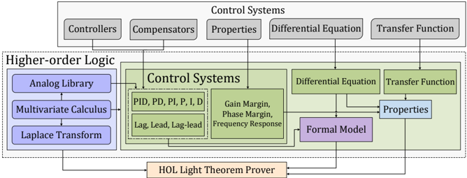
In this paper, we present a framework to conduct the formal analysis of dynamical characteristics of a linear control system using higher-order-logic theorem proving. The main idea behind the proposed framework, depicted in Fig. 1, is to formalize all the foundational components of a linear control system to facilitate formal modeling and reasoning about linear control systems within the sound core of a theorem prover. For this purpose, we built upon the higherorder-logic formalizations of Multivariable calculus [9] and a library of analog components, like resistor, capacitor and inductor [21]. We present a new formalization of Laplace transform , which includes the formal verification of some of its frequently used properties in reasoning about the transfer function of an n -order system. We also formalized some widely used characteristics of linear control systems , such as frequency response, gain margin and phase margin, which can be used for the stability analysis of a linear control system. Moreover, we formalize the active realizations of various controllers , such as ProportionalIntegral-Derivative (PID), Proportional-Integral (PI), Proportional-Derivative (PD), Proportional (P), Integral (I) and Derivative (D) and various active and passive compensators , such as lag, lead and lag-lead.
The proposed framework, depicted in Fig. 1, allows us to build a formal model of the given linear control system, based on the active realizations of its
Fig. 1: Proposed Framework
<details>
<summary>Image 1 Details</summary>
### Visual Description
## Diagram: Control Systems Overview
### Overview
The image is a diagram illustrating the relationships between different components in control systems, higher-order logic, and a theorem prover. It shows how various elements like controllers, compensators, differential equations, and transfer functions are interconnected and how they relate to formal models and properties.
### Components/Axes
The diagram is structured into several key components:
* **Top Layer:** Contains "Controllers", "Compensators", "Properties", "Differential Equation", and "Transfer Function". These are represented as gray rounded rectangles.
* **Middle Layer (Higher-order Logic):** Enclosed in a dashed-line rectangle, this section contains "Analog Library", "Multivariate Calculus", "Laplace Transform" (all in blue), "Control Systems" (in green), "PID, PD, PI, P, I, D" and "Lag, Lead, Lag-lead" (within the "Control Systems" box), "Gain Margin, Phase Margin, Frequency Response" (also within the "Control Systems" box), "Differential Equation", "Transfer Function" (both in green), "Formal Model" (in purple), and "Properties" (in blue).
* **Bottom Layer:** Contains "HOL Light Theorem Prover" (in orange).
### Detailed Analysis or ### Content Details
* **Top Layer:**
* "Controllers": Located at the top-left.
* "Compensators": Located to the right of "Controllers".
* "Properties": Located to the right of "Compensators".
* "Differential Equation": Located to the right of "Properties".
* "Transfer Function": Located at the top-right.
* **Middle Layer (Higher-order Logic):**
* "Analog Library": Located at the left, within the "Higher-order Logic" box.
* "Multivariate Calculus": Located below "Analog Library".
* "Laplace Transform": Located below "Multivariate Calculus".
* "Control Systems": A large green box in the center, containing:
* "PID, PD, PI, P, I, D": Located within the "Control Systems" box.
* "Lag, Lead, Lag-lead": Located below "PID, PD, PI, P, I, D" within the "Control Systems" box.
* "Gain Margin, Phase Margin, Frequency Response": Located to the right of the other two within the "Control Systems" box.
* "Differential Equation": Located to the right of "Control Systems".
* "Transfer Function": Located to the right of "Differential Equation".
* "Formal Model": Located below "Differential Equation" and "Transfer Function".
* "Properties": Located to the right of "Formal Model".
* **Bottom Layer:**
* "HOL Light Theorem Prover": Located at the bottom, spanning the width of the diagram.
* **Connections:**
* Arrows connect "Analog Library", "Multivariate Calculus", and "Laplace Transform" to "Control Systems".
* Arrows connect "Control Systems" to "Differential Equation", "Transfer Function", and "Formal Model".
* Arrows connect "Differential Equation" and "Transfer Function" to "Properties".
* Arrows connect "Controllers", "Compensators", "Properties", "Differential Equation", and "Transfer Function" from the top layer to the "Control Systems" box in the middle layer.
* Arrows connect "Formal Model" and "Properties" to "HOL Light Theorem Prover".
* Arrows connect "Analog Library", "Multivariate Calculus", and "Laplace Transform" to "HOL Light Theorem Prover".
### Key Observations
* The diagram illustrates a hierarchical structure, with high-level control system components at the top, lower-level logic and mathematical tools in the middle, and a theorem prover at the bottom.
* The "Control Systems" box in the middle layer acts as a central hub, connecting various elements.
* The "HOL Light Theorem Prover" receives input from multiple sources, suggesting its role in verifying or analyzing the control systems.
### Interpretation
The diagram represents a workflow or architecture for designing and verifying control systems. It suggests that higher-order logic and mathematical tools are used to model and analyze control systems, and the "HOL Light Theorem Prover" is used to formally verify the properties of these systems. The connections between the components indicate the flow of information and dependencies between different stages of the design and verification process. The diagram highlights the importance of formal methods in ensuring the correctness and reliability of control systems.
</details>
controllers and compensators, the passive realizations of compensators and differential equations. Moreover, it also allows to formalize the behavior of the
given linear control system in terms of its differential equation, transfer function specification and its properties, such as phase margin, frequency response and gain margin. We can then use these formalized models and properties to verify an implication relationship between them, i.e., model implies its specification. In order to demonstrate the effectiveness of our proposed formalization, we formalize the control system of an unmanned free-swimming submersible vehicle [15]. We have used the HOL Light theorem prover [8] for the proposed formalization in order to build upon its multivariable calculus theories. We have also developed a tactic that can be used to automatically verify the transfer function of any control system up to 20 th order . This tactic was found to be very handy in the formal analysis of the unmanned submersible vehicle.
## 2 Multivariable Calculus Theories in HOL Light
An N-dimensional vector is formalized in the multivariable theory of HOL Light as a R N column matrix of real numbers [9]. All of the multivariable calculus theorems are verified for functions with an arbitrary data-type R N → R M .
A complex number is defined as a 2-dimensional vector, i.e., a R 2 matrix.
```
Definition 1. |- \a. Cx a = complex (a, &0)
|- ii = complex (&0, &1)
```
Cx : R → R 2 is a type casting function that accepts a real number and returns its corresponding complex number with the imaginary part equal to zero, where the & operator type casts a natural number to its corresponding real number. Similarly, ii (iota) represents a complex number having the real part equal to zero and the magnitude of the imaginary part equal to 1.
```
Definition 2. |- \z. Re z = z$1
```
The function Re accepts a complex number (2-dimensional vector) and returns its real part. Here, the notation z $ i represents the i th component of vector z . Similarly, Im takes a complex number and returns its imaginary part. The function lift accepts a variable of type R and maps it to a 1-dimensional vector with the input variable as its single component. Similarly, drop takes a 1-dimensional vector and returns its single element as a real number.
```
Definition 3. |- \x. exp x = Re (cexp (Cx x))
```
The complex exponential and real exponentials are represented as cexp : R 2 → R 2 and exp : R → R in HOL Light, respectively.
```
Definition 4. - \forall f i. integral i f = (@y. (f has integral y) i)
\verbatim
\f a f i. real integral i f = (@y. (f has real integral y) i)
```
The function integral represents the vector integral and is defined using the Hilbert choice operator @ in the functional form. It takes the integrand function f , having an arbitrary type R N → R M , and a vector-space i : R N → B , which defines the region of convergence as B represents the boolean data type, and returns a vector R M , which is the integral of f on i . The function has integral represents the same relationship in the relational form. Similarly, the function real integral accepts the integrand function f : R → R and a set of real numbers i : R → B and returns the real-valued integral of function f over i . The region of integration, for both of the above integrals can be defined to be bounded by a vector interval [ a, b ] or real interval [ a, b ] using the HOL Light functions interval [ a , b ] and real interval [ a , b ], respectively.
## Definition 5.
∀ f net. vector derivative f net = (@f'.(f has vector derivative f') net)
The function vector derivative takes a function f : R 1 → R M and a net : R 1 → B , which defines the point at which f has to be differentiated, and returns a vector of data-type R M , which represents the differential of f at net . The function has vector derivative defines this relationship in the relational form.
$$D e f n i t i o n 6 . \, \vdash \forall f \, n e t . \, l i m \, n e t \, f = ( \mathbb { O } _ { 1 } . \, ( f \to 1 ) \, n e t )$$
The function lim accepts a net with elements of arbitrary data-type A and a function f : A → R M and returns l of data-type R M , i.e., the value to which f converges at the given net .
## 3 Formalization of Laplace Transform
Mathematically, Laplace transform is defined for a function f : R 1 → C as [4]:
$$\mathcal { L } [ f ( t ) ] = F ( s ) = \int _ { 0 } ^ { \infty } f ( t ) e ^ { - s t } d t , \, s \epsilon \, \mathbb { C } & & ( 1 )$$
We formalize Equation 1 in HOL Light as follows:
$$\text {Definition 7.} \, \vdash \forall s f . l a p l a c e t r a n s t o r f i s = \\ \text {integral } \{ t | \& 0 \leq d r o p \} ( \lambda t . c x p \left ( - ( s * C x \, ( d r o p \, t ) ) \right ) * f \, t )$$
The function laplace transform accepts a complex-valued function f : R 1 → R 2 and a complex number s and returns the Laplace transform of f as represented by Equation 1. In the above definition, we used the complex exponential function cexp : R 2 → R 2 because the return data-type of the function f is R 2 . Here, the data-type of t is R 1 and to multiply it with the complex number s , it is first converted into a real number by using drop and then it is converted to data-type R 2 using Cx . Next, we use the vector function integral (Definition 4) to integrate the expression f ( t ) e -iωt over the positive real line since the datatype of this expression is R 2 . The region of integration is { t | &0 <= drop t } , which represents the positive real line. Laplace transform was earlier formalized using a limiting process as [20]:
```
|- \s f. laplace f s = lim at posinfinity (\b. integral
(interval [lift (&0), lift b]) (\t. cexp (--(s * Cx (drop t))) * f t))
```
However, the HOL Light definition of the integral function implicitly encompasses infinite limits of integration. So, our definition covers the region of integration, i.e., [0 , ∞ ), as { t | &0 <= drop t } and is equivalent to the definition given in [20]. However, our definition considerably simplifies the reasoning process in the verification of Laplace transform properties since it does not involve the notion of limit.
The Laplace transform of a function f exists, if f is piecewise smooth and is of exponential order on the positive real line [4,19]. A function is said to be piecewise smooth on an interval if it is piecewise differentiable on that interval.
```
Definition 8. + \s f. laplace exists f s <=>
( \b . f piecewise differentiable on interval [lift (&0),lift b] ) ^
( \m a. Re s > drop a \^ exp order cond f M a)
```
The function exp order cond in the above definition represents the exponential order condition necessary for the existence of the Laplace transform [20,4]:
```
Definition 9. |- \f M a. exp order f M a <=> &0 < M ^ { * } \\ ( \forall t . &0 <= t \Rightarrow n o r m ( f ( l i f t ) ) \leq M * \exp ( d r o p a * t ) )
```
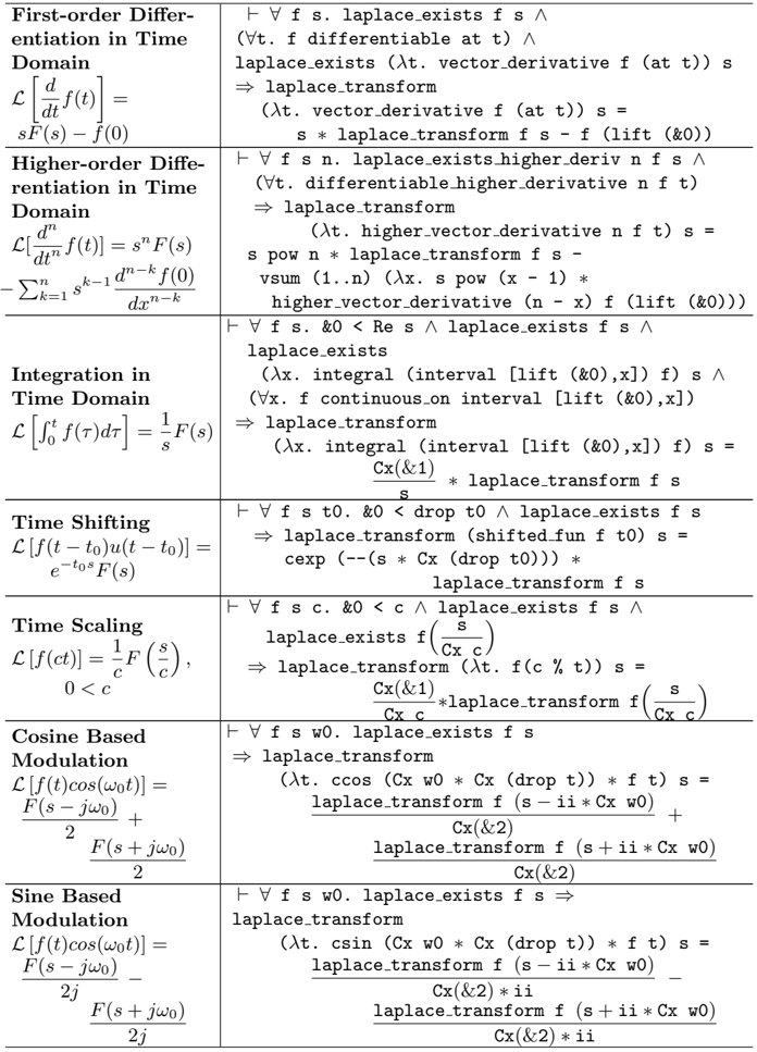
We used Definitions 7, 8 and 9 to formally verify some of the classical properties of Laplace transform, given in Table 1. The properties namely linearity, frequency shifting, differentiation and integration were already verified using the formal definition of the Laplace transform [20]. We formally verified these using our new definition of the Laplace transform. Moreover, we formally verified some new properties, such as, time shifting, time scaling, cosine and sine-based modulations and the Laplace transform of a n -order differential equation. The assumptions of these theorems describe the existence of the corresponding Laplace transforms. For example, the predicate laplace exists higher deriv in the theorem corresponding to the n -order differential equation ensures that the La-
Table 1: Properties of Laplace Transform
| Property | Formalized Form |
|---------------------------------------------------------|---------------------------------------------------------------------------------------------------------------------------------------------------------------------------------|
| Integrability e - st f ( t ) integrable on [0 , ∞ ) | ∀ f s. laplace exists f s ⇒ ( λ t. cexp (--(s ∗ Cx (drop t))) ∗ f t) integrable on { t | &0 <= drop t } |
| Linearity L [ αf ( t )+ βg ( t )] = αF ( s )+ βG ( s ) | ∀ f g s a b. laplace exists f s ∧ laplace exists g s ⇒ laplace transform ( λ t. a ∗ f t + b ∗ g t) s a ∗ laplace transform f s + b ∗ laplace transform g s |
| Frequency Shifting L [ e s 0 t f ( t )] = F ( s - s 0 ) | ∀ f s s0. laplace exists f s ⇒ laplace transform ( λ t. cexp (s0 ∗ Cx (drop t)) ∗ f t) s = laplace transform f (s - s0) |
<details>
<summary>Image 2 Details</summary>
### Visual Description
## Laplace Transform Properties: Time Domain Operations
### Overview
The image presents a table summarizing several properties of the Laplace transform related to operations performed in the time domain. It includes formulas for differentiation, integration, time shifting, time scaling, and modulation (cosine and sine). Each property is presented with its corresponding Laplace transform and any necessary conditions.
### Components/Axes
The table is structured with the following columns:
1. **Operation Description**: Describes the operation performed on the function in the time domain (e.g., "First-order Differentiation in Time Domain").
2. **Laplace Transform**: Provides the formula for the Laplace transform of the modified function, denoted as L[f(t)] = F(s).
3. **Conditions/Mathematical Expressions**: Specifies the conditions under which the property holds, often involving quantifiers and logical statements.
### Detailed Analysis or ### Content Details
Here's a breakdown of each row:
1. **First-order Differentiation in Time Domain**
* **Description**: Deals with the Laplace transform of the derivative of a function.
* **Laplace Transform**: L[d/dt f(t)] = sF(s) - f(0)
* **Conditions**: ∀ f s. laplace\_exists f s ∧ (∀t. f differentiable at t) ∧ laplace\_exists (λt. vector\_derivative f (at t)) s ⇒ laplace\_transform (λt. vector\_derivative f (at t)) s = s \* laplace\_transform f s - f (lift (&0))
2. **Higher-order Differentiation in Time Domain**
* **Description**: Deals with the Laplace transform of the nth derivative of a function.
* **Laplace Transform**: L[d^n/dt^n f(t)] = s^n F(s) - Σ{k=1 to n} s^(k-1) d^(n-k)/dx^(n-k) f(0)
* **Conditions**: ∀ f s n. laplace\_exists\_higher\_deriv n f s ∧ (∀t. differentiable higher\_derivative n f t) ⇒ laplace\_transform (λt. higher\_vector\_derivative n f t) s = s pow n \* laplace\_transform f s - vsum (1..n) (λx. s pow (x - 1) \* higher\_vector\_derivative (n - x) f (lift (&0)))
3. **Integration in Time Domain**
* **Description**: Deals with the Laplace transform of the integral of a function.
* **Laplace Transform**: L[∫{0 to t} f(τ) dτ] = (1/s) F(s)
* **Conditions**: ∀ f s. &0 < Re s ∧ laplace\_exists f s ∧ laplace\_exists (λx. integral (interval [lift (&0),x]) f) s ∧ (∀x. f continuous\_on interval [lift (&0),x]) ⇒ laplace\_transform (λx. integral (interval [lift (&0),x]) f) s = Cx(&1)/s \* laplace\_transform f s
4. **Time Shifting**
* **Description**: Deals with the Laplace transform of a time-shifted function.
* **Laplace Transform**: L[f(t - t0)u(t - t0)] = e^(-t0s) F(s)
* **Conditions**: ∀ f s t0. &0 < drop t0 ∧ laplace\_exists f s ⇒ laplace\_transform (shifted\_fun f t0) s = cexp (-- (s \* Cx (drop t0))) \* laplace\_transform f s
5. **Time Scaling**
* **Description**: Deals with the Laplace transform of a time-scaled function.
* **Laplace Transform**: L[f(ct)] = (1/c) F(s/c), 0 < c
* **Conditions**: ∀ f s c. &0 < c ∧ laplace\_exists f s ∧ laplace\_exists f(s/Cx c) ⇒ laplace\_transform (λt. f(c % t)) s = Cx(&1)/(Cx c) \* laplace\_transform f(s/Cx c)
6. **Cosine Based Modulation**
* **Description**: Deals with the Laplace transform of a function multiplied by a cosine.
* **Laplace Transform**: L[f(t)cos(ω0t)] = F(s - jω0)/2 + F(s + jω0)/2
* **Conditions**: ∀ f s w0. laplace\_exists f s ⇒ laplace\_transform (λt. ccos (Cx w0 \* Cx (drop t)) \* f t) s = laplace\_transform f (s - ii \* Cx w0) / Cx(&2) + laplace\_transform f (s + ii \* Cx w0) / Cx(&2)
7. **Sine Based Modulation**
* **Description**: Deals with the Laplace transform of a function multiplied by a sine.
* **Laplace Transform**: L[f(t)cos(ω0t)] = F(s - jω0)/(2j) - F(s + jω0)/(2j)
* **Conditions**: ∀ f s w0. laplace\_exists f s ⇒ laplace\_transform (λt. csin (Cx w0 \* Cx (drop t)) \* f t) s = laplace\_transform f (s - ii \* Cx w0) / (Cx(&2) \* ii) - laplace\_transform f (s + ii \* Cx w0) / (Cx(&2) \* ii)
### Key Observations
* The table provides a concise summary of how time-domain operations affect the Laplace transform of a function.
* Each property is accompanied by conditions that must be met for the property to hold.
* The modulation properties (cosine and sine) involve complex numbers (j or ii, representing the imaginary unit).
### Interpretation
The table serves as a reference for engineers and scientists who use Laplace transforms to analyze and solve differential equations and other problems in linear systems. It demonstrates how operations in the time domain (differentiation, integration, shifting, scaling, and modulation) translate into corresponding operations in the s-domain (Laplace domain), which can simplify the analysis and solution of complex systems. The conditions specified for each property ensure the validity of the transform.
</details>
| First-order Differ- entiation in Time Domain L [ d dt f ( t ) ] = sF ( s ) - f (0) | ∀ f s. laplace exists f s ∧ ( ∀ t. f differentiable at t) ∧ laplace exists ( λ t. vector derivative f (at t)) s ⇒ laplace transform ( λ t. vector derivative f (at t)) s = |
|------------------------------------------------------------------------------------------|----------------------------------------------------------------------------------------------------------------------------------------------------------------------------------------------------------------------------------------------------------------------------------|
| Higher-order Diffe- rentiation in Time Domain L [ d n n f ( t )] = s n F ( s ) | s ∗ laplace transform f s - f (lift (&0)) ∀ f s n. laplace exists higher deriv n f s ∧ ( ∀ t. differentiable higher derivative n f t) |
| dt - ∑ n k =1 s k - 1 d n - k f (0) dx n - k | ⇒ laplace transform ( λ t. higher vector derivative n f t) s = s pow n ∗ laplace transform f s - vsum (1..n) ( λ x. s pow (x - 1) ∗ higher vector derivative (n - x) f (lift (&0))) |
| Integration in Time Domain L [ ∫ t 0 f ( τ ) dτ ] = 1 s F ( s ) | ∀ f s. &0 < Re s ∧ laplace exists f s ∧ laplace exists ( λ x. integral (interval [lift (&0),x]) f) s ∧ ( ∀ x. f continuous on interval [lift (&0),x]) ⇒ laplace transform ( λ x. integral (interval [lift (&0),x]) f) s = Cx (& 1 ) ∗ laplace transform f s |
| Time Shifting L [ f ( t - t 0 ) u ( t - t 0 )] = e - t 0 s F ( s ) | s ∀ f s t0. &0 < drop t0 ∧ laplace exists f s ⇒ laplace transform (shifted fun f t0) s = cexp (--(s ∗ Cx (drop t0))) ∗ laplace transform f s |
| Time Scaling L [ f ( ct )] = 1 c F ( s c ) , 0 < c | ∀ f s c. &0 < c ∧ laplace exists f s ∧ laplace exists f ( s Cx c ) ⇒ laplace transform ( λ t. f(c % t)) s = Cx (& 1 ) Cx c ∗ laplace transform f ( s Cx c ) |
| Cosine Based Modulation L [ f ( t ) cos ( ω 0 t )] = F ( s - jω 0 ) 2 + F ( s + jω 0 ) 2 | ∀ f s w0. laplace exists f s ⇒ laplace transform ( λ t. ccos (Cx w0 ∗ Cx (drop t)) ∗ f t) s = laplace transform f ( s - ii ∗ Cx w0 ) Cx (& 2 ) + laplace transform f ( s + ii ∗ Cx w0 ) Cx (& 2 ) |
| Sine Based Modulation L [ f ( t ) cos ( ω 0 t )] = F ( s - jω 0 ) 2 j - F ( s + jω 0 ) | ∀ f s w0. laplace exists f s ⇒ laplace transform ( λ t. csin (Cx w0 ∗ Cx (drop t)) ∗ f t) s = laplace transform f ( s - ii ∗ Cx w0 ) Cx (& 2 ) ∗ ii - laplace transform f ( s + ii ∗ Cx w0 ) |
| n -order Differ- ential Equation L ( ∑ n k =0 α k d k y dt k ) = F ( s ) ∑ n k =0 α k s k - ∑ n k =0 ∑ k i =1 s i - 1 d k - i f (0) dt k - i | ∀ f lst s n. laplace exists higher deriv n f s ∧ ( ∀ t. differentiable higher derivative n f t) ⇒ laplace transform ( λ t. diff eq n order n lst f t) s = laplace transform f s ∗ vsum (0..n) ( λ k. EL k lst ∗ s pow k) - vsum (0..n) ( λ k. EL k lst ∗ vsum (1..k) ( λ i. s pow (i - 1) ∗ higher vector derivative (k - i) f (lift (&0)))) |
|------------------------------------------------------------------------------------------------------------------------------------------------|---------------------------------------------------------------------------------------------------------------------------------------------------------------------------------------------------------------------------------------------------------------------------------------------------------------------------------------------------------------------|
place of all the derivatives up to the n th order of the function f exist. Similarly, the predicate differentiable higher derivative provides the differentiability of the function f and its higher derivatives up to the n th order. The verification of these properties not only ensures the correctness of our definitions but also plays a vital role in minimizing the user effort in reasoning about Laplace transform based analysis of systems, as will be depicted in Sections 4 and 5 of this paper.
The generalized linear differential equation describes the input-output relationship for a generic n -order linear control system [15]:
$$\sum _ { k = 0 } ^ { n } \alpha _ { k } \frac { d ^ { k } } { d t ^ { k } } y ( t ) = \sum _ { k = 0 } ^ { m } \beta _ { k } \frac { d ^ { k } } { d t ^ { k } } x ( t ) , \quad m \leq n \quad ( 2 )$$
where y ( t ) is the output and x ( t ) is the input to the system. The constants α k and β k are the coefficients of the output and input differentials with order k , respectively. The greatest index n of the non-zero coefficient α n determines the order of the underlying system. The corresponding transfer function is obtained by setting the initial conditions equal to zero [15]:
$$\frac { Y ( s ) } { X ( s ) } = \frac { \sum _ { k = 0 } ^ { m } \beta _ { k } s ^ { k } } { \sum _ { k = 0 } ^ { n } \alpha _ { k } s ^ { k } } \quad ( 3 )$$
We verified the transfer function, given in Equation 3, for the generic n-order linear control system as the following HOL Light theorem.
## Theorem 1. ∀ y x m n inlst outlst s.
```
Theorem 1. + \y x m n inlst outlst s.
( \forall t. differentiable higher deriv m n x y t) ^
laplace exists of higher deriv m n x y s ^ zero init conditions m n x y ^
diff eq n order sys m n inlst outlst x y ^
~(laplace transform x s = Cx (&0)) ^
~(vsum (0..n) ( \lambda. t. EL t outlst * s pow t) = Cx (&0))
=> laplace transform y s = vsum (0..m) ( \lambda.t. EL t inlst * s pow t)
:= laplace transform x s = vsum (0..n) ( \lambda.t. EL t outlst * s pow t)
```
The first assumption ensures that the functions y and x are differentiable up to the n th and m th order, respectively. The next assumption represents the Laplace transform existence condition up to the n th order derivative of function y and m th order derivative of the function x . The next assumption models the zero initial conditions for both of the functions y and x , respectively. The next assumption represents the formalization of Equation 2 and the last two assumptions provide
the conditions for the design of a reliable linear control system. Finally, the conclusion of the above theorem represents the transfer function given by Equation 3. The verification of this theorem is very useful as it allows to automate the verification of the transfer function of any linear control system as described in Sections 4 and 5 of the paper. The formalization, described in this section, took around 2000 lines of HOL Light code [17] and around 130 man-hours.
## 4 Formalization of Linear Control Systems Foundations
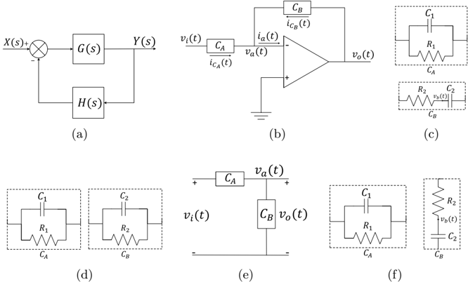
A general closed-loop control system is depicted in Fig. 2a. Here, X ( s ) and Y ( s ) represent the Laplace transforms of the time domain input x ( t ) and the output y ( t ), respectively. G ( s ) and H ( s ) represent the forward path and the feedback path transfer functions, respectively. Similarly, G ( s ) H ( s ) is the open loop transfer function of the system and Y ( s ) /X ( s ) is the closed loop transfer function [7]. Table 2 presents the formalization of the frequency response, phase margin and gain margin of this control system. These properties are used to study the dynamics of a linear control system in the frequency domain and to perform its stability analysis.
The frequency response is used to analyze the dynamics of the system by studying the impact of different frequency components on the intended behaviour of the given linear control system. We also formally verified the frequency response of a generic n -order system based on assumptions that are very similar to the ones used for Theorem 1.
Table 2: Properties of Linear Control Systems
| Property | Formalized Form |
|------------------------------------------------------------------------------------------------------------|----------------------------------------------------------------------------------------------------------------------------------------------------------------------------------------------------------------------------------------------------------------------------------------------------------------------------------------------------------------------------------------------------------|
| Frequency Response M ( jω ) = M ( s ) | ( jω ) = Y ( s ) X ( s ) ∣ ∣ ∣ ∣ ∣ ( jω ) = Y ( jω ) X ( jω ) | ∀ y x w. frequency response x y w = laplace transform y ( ii ∗ Cx w ) laplace transform x ( ii ∗ Cx w ) |
| Frequency Response of an n -order System Y ( jω ) X ( jω ) = ∑ m k =0 β k ( jω ) k ∑ n k =0 α k ( jω ) k | ∀ y x m n inlst outlst s. ( ∀ t. differentiable higher deriv m n x y t) ∧ laplace exists of higher deriv m n x y w ∧ zero init conditions m n x y ∧ diff eq n order sys m n inlst outlst y x ∧ non zero denom cond n x w outlst ⇒ frequency response x y w = vsum ( 0 .. m ) ( λ t . EL t inlst ∗ ( ii ∗ Cx w ) pow t ) vsum ( 0 .. n ) ( λ t . EL t outlst ∗ ( ii ∗ Cx w ) pow t ) |
| Phase Margin [ ∠ G ( jω ) H ( jω )] ω = ω gc + 180 o | ∀ g h wgc. phase margin g h wgc = pi + Arg (g (ii ∗ Cx wgc) ∗ h (ii ∗ Cx wgc)) |
| Gain Margin [ 20 log 10 ∣ ∣ ∣ G ( jω ) H ( jω ) ∣ ∣ ∣ ω = ω pc ] dB | ∀ g h wpc. gain margin db g h wpc = &20 ∗ log ( norm ( g ( ii ∗ Cx wpc ) ∗ h ( ii ∗ Cx wpc ))) log (& 10 ) |
Phase margin and gain margin provide useful information about controlling the stability of the system [7]. Phase margin represents 180 o shifted phase angle of the open loop transfer function evaluated at the gain crossover frequency ( ω gc ), which is the frequency at which the magnitude of the open loop transfer function is equal to 0 dB. The gain margin represents the magnitude of the open loop transfer function evaluated at the phase crossover frequency ( ω pc ), which is the frequency at which the resultant phase curve of the open loop gain has a phase of 180 o . In our formal definitions of these notions, the function Arg(z) represents the argument of a complex number z .
Fig. 2: Control Systems Foundations (a) Closed Loop Control System (b) Generic Active Realization of Controller (c) PID Configuration (d) Lag/lead Compensator Configuration (e) Generic Passive Realization of Compensator (f) Lag-lead Compensator Configuration
<details>
<summary>Image 3 Details</summary>
### Visual Description
## Circuit Diagrams: Control System and Op-Amp Configurations
### Overview
The image presents a collection of circuit diagrams and block diagrams related to control systems and operational amplifier (op-amp) configurations. It includes a feedback control system, an op-amp circuit with input and feedback components, and several variations of RC circuits.
### Components/Axes
* **(a) Feedback Control System:**
* **X(s):** Input signal
* **Y(s):** Output signal
* **G(s):** Forward path transfer function
* **H(s):** Feedback path transfer function
* Summing junction with positive and negative inputs.
* **(b) Op-Amp Circuit:**
* **v<sub>i</sub>(t):** Input voltage
* **v<sub>a</sub>(t):** Voltage at the inverting input of the op-amp
* **v<sub>o</sub>(t):** Output voltage
* **C<sub>A</sub>:** Input capacitor
* **i<sub>CA</sub>(t):** Current through C<sub>A</sub>
* **C<sub>B</sub>:** Feedback capacitor
* **i<sub>CB</sub>(t):** Current through C<sub>B</sub>
* Op-amp symbol with inverting (-) and non-inverting (+) inputs. The non-inverting input is grounded.
* **(c), (d), (e), (f) RC Circuits:**
* **R<sub>1</sub>, R<sub>2</sub>:** Resistors
* **C<sub>1</sub>, C<sub>2</sub>:** Capacitors
* **C<sub>A</sub>, C<sub>B</sub>:** Capacitors associated with circuit A and B respectively.
* **v<sub>b</sub>(t):** Voltage across the R2-C2 combination in (c) and (f).
* **v<sub>i</sub>(t):** Input voltage in (e).
* **v<sub>o</sub>(t):** Output voltage in (e).
* **v<sub>a</sub>(t):** Voltage at the junction of CA and CB in (e).
### Detailed Analysis or ### Content Details
* **(a) Feedback Control System:** A standard negative feedback control system is depicted. The input signal X(s) is compared with the feedback signal H(s) * Y(s). The error signal is then fed into the forward path transfer function G(s) to produce the output Y(s).
* **(b) Op-Amp Circuit:** An op-amp is configured with an input capacitor C<sub>A</sub> and a feedback capacitor C<sub>B</sub>. The input voltage v<sub>i</sub>(t) is applied through C<sub>A</sub> to the inverting input of the op-amp. The output voltage v<sub>o</sub>(t) is fed back through C<sub>B</sub> to the inverting input. The non-inverting input is grounded.
* **(c) RC Circuits:** Two parallel RC circuits are shown, labeled C<sub>A</sub> and C<sub>B</sub>. C<sub>A</sub> consists of a capacitor C<sub>1</sub> in parallel with a resistor R<sub>1</sub>. C<sub>B</sub> consists of a capacitor C<sub>2</sub> in series with a resistor R<sub>2</sub>, and the voltage across the R2-C2 combination is labeled v<sub>b</sub>(t).
* **(d) RC Circuits:** Two parallel RC circuits are shown in series, labeled C<sub>A</sub> and C<sub>B</sub>. C<sub>A</sub> consists of a capacitor C<sub>1</sub> in parallel with a resistor R<sub>1</sub>. C<sub>B</sub> consists of a capacitor C<sub>2</sub> in parallel with a resistor R<sub>2</sub>.
* **(e) RC Circuits:** A series RC circuit is shown, with C<sub>A</sub> in series with C<sub>B</sub>. C<sub>A</sub> is a capacitor, and C<sub>B</sub> is a capacitor. The input voltage v<sub>i</sub>(t) is applied to the series combination, and the output voltage v<sub>o</sub>(t) is taken across C<sub>B</sub>. The voltage at the junction of CA and CB is labeled v<sub>a</sub>(t).
* **(f) RC Circuits:** Two RC circuits are shown, labeled C<sub>A</sub> and C<sub>B</sub>. C<sub>A</sub> consists of a capacitor C<sub>1</sub> in parallel with a resistor R<sub>1</sub>. C<sub>B</sub> consists of a capacitor C<sub>2</sub> in series with a resistor R<sub>2</sub>, and the voltage across the R2-C2 combination is labeled v<sub>b</sub>(t).
### Key Observations
* The diagrams illustrate fundamental concepts in control systems and analog circuit design.
* The op-amp circuit in (b) likely represents an inverting amplifier configuration with capacitive input and feedback.
* The RC circuits in (c), (d), (e), and (f) demonstrate different arrangements of resistors and capacitors, which can be used for filtering, impedance matching, or other signal processing functions.
### Interpretation
The image provides a visual representation of basic control system principles and op-amp circuit configurations. The feedback control system demonstrates how negative feedback is used to regulate a system's output. The op-amp circuit shows how capacitors can be used to shape the frequency response of an amplifier. The RC circuits illustrate the versatility of resistors and capacitors in creating various signal processing functions. The different arrangements of resistors and capacitors in (c), (d), (e), and (f) would result in different frequency responses and impedance characteristics.
</details>
The controllers form the most vital part of any control system as they are mainly responsible for the correct operation of every component of the underlying system. Controllers are modeled using their active realizations based on an electrical circuit, which comprises of an inverting operational amplifier (op-amp) with unity gain, and two components, i.e., C A and C B , which are shown as rectangular boxes in Fig. 2b. The boxes C A and C B contain different configurations of the passive components, i.e., resistors and capacitors [16]. By making an appropriate choice of these passive components, we obtain various controllers, such as P, I, D, PI, PD, PID [15]. For the analysis of these controllers, we first need to formalize them in higher-order logic. This step requires a formal library of analog components [21,17], describing the voltage-current relationships of resistor, capacitors and inductors, and the KCL and KVL, which model the currents and voltages in an electrical circuit.
The PID controller, depicted in Fig. 2c, can be formalized as follows:
```
Definition 10. |- \C1 R1 Vi R2 C2 Vo Vb Va.
pid controller implem Vi Vo Va Vb C1 C2 R1 R2 <>
( \t. &0 < drop t => kcl [\t. capacitor current C1 (\t. Vi t - Va t) t;
\t. resistor current R1 (\t. Vi t - Va t) t;
\t. resistor current R2 (\t. Vb t - Va t) t] ^
( \t. &0 < drop t => kcl [\t. resistor current R2 (\t. Va t - Vb t) t;
\t. capacitor current C2 (\t. Vo t - Vb t) t] ^
( \t. &0 < drop t => Va t = Cx (&0))
```
where Vi and Vo are the input and the output voltages, respectively, having data type R 1 → C , and Va and Vb are the voltages at nodes a and b , respectively. The functions resistor current and capcitor current are the currents across the resistor and capacitor, respectively. The function kcl accepts a list of currents across the components of the circuit and a time variable t and returns the predicate that guarantees that the sum of all the currents leaving a particular node at time t is zero. The first conjunct of the above definition represents the application of KCL across node a . Similarly, the second conjunct models the KCL at node b , whereas the last conjunct provides the voltage across the non-inverting input of the op-amp using the virtual ground condition, as shown in Fig. 2b. We also develop a simplification tactic KCL SIMP TAC , which simplifies the implementations of the PID controller as well as other controllers and compensators. The details can be found in [17].
Next, we model the dynamical behaviour of the PID controller using the n -order differential equation:
```
Definition 11. ! R1 R2 C1 C2. inlst pid contr R1 R2 C1 C2 =
[--Cx (&1); --Cx (R2 * C2 + R1 * C1); --Cx (R1 * R2 * C1 * C2)]
! ! R1 C2. outlst pid contr R1 C2 = [Cx (&0); Cx (R1 * C2)]
! ! Vo R1 R2 C1 C2 Vi t. pid controller behav spec R1 R2 C1 C2 Vi Vo t <>
diff eq n order 1 (outlst pid contr R1 C2) Vo t =
diff eq n order 2 (inlst pid contr R1 R2 C1 C2) Vi t
```
We verified the behavioural specification based on the implementation of the PID controller as the following theorem:
```
Theorem 2. - ∀ R1 R2 C1 C2 Vi Va Vb Vo t. &0 < R1 ∧ &0 < R2 ∧
&0 < C1 ∧ &0 < C2 ∧ (∀t. differentiable higher derivative Vi Vo Vb t) ∧
pid controller implem Vi Vo Va Vb C1 C2 R1 R2
⇒ (&0 < drop t ⇒ pid controller behav spec R1 R2 C1 C2 Vi Vo t)
```
The first four assumptions model the design requirement for the underlying system. The next assumption provides the differentiability of the higher-order derivatives of Vi , Vo and Vb up to the order 1, 2 and 2, respectively. The last assumption presents the implementation for the PID controller. Finally, the conclusion presents its behavioral specification. We also develop a simplification tactic DIFF SIMP TAC , which simplifies the behavioural specifications of the PID controller as well as the other controllers and compensators [17].
Next, we verified the transfer function of the PID controller as follows:
```
Theorem 3. ⊢ \ R1 R2 C1 C2 Vi Vo s t. &0 < R1 ^ \& 0 < R2 ^ \& 0 < C1 ^
~(laplace transform Vi s = Cx (&0)) ^ \sim (Cx R1 * Cx C2 * s = Cx (&0)) ^
&0 < C2 ^ \wedge ( \forall t. differentiable higher derivative Vi Vo t) ^
laplace exists higher deriv Vi Vo s ^ zero initial conditions Vi Vo ^
( \forall t. pid controller behav spec R1 R2 C1 C2 Vi Vo t)
=> laplace transform Vo s =
laplace transform Vi s
--(Cx(R1 * C1 * R2 * C2) * s pow 2 + (Cx(R2 * C2) + Cx(C1 * R1)) * s + Cx(&1))
```
Cx ( R1 ∗ C2 ) ∗ s
The first six assumptions present the design requirements for the underlying system. The next two assumptions provide the differentiability and the Laplace existence condition for the higher-order derivatives of Vi and Vo up to the order 2 and 1, respectively. The next assumption models the zero initial conditions for the voltage functions Vi and Vo . The last assumption presents the behavioural specification of the PID controller. Finally, the conclusion of Theorem 3 presents its required transfer function. By judicious selection of the configuration of passive components, we obtain various controllers, such as P, I, D, PI, PD and perform the above-mentioned analysis for all of them.
Compensators are widely used in control systems, to improve their frequency response, steady-state error and the stability and hence, act as a fundamental block of a control system. Like controllers, the compensators are also modeled using their active realizations. A compensator uses the same analog circuit, which is used for the controllers, presented in Fig. 2b, by making an appropriate choice of the passive components C A and C B , as shown in Fig. 2d. It acts as a lag-compensator under the condition R 2 C 2 > R 1 C 1 , whereas for the case of R 1 C 1 > R 2 C 2 , it acts as a lead-compensator. The configurations of the passive components for the controllers and compensators, and their formalization is presented in [17].
Compensators are also modeled using their passive realizations based on an electrical circuit, which comprises of two components, i.e., C A and C B , which are shown as rectangular boxes in Fig. 2e. The boxes C A and C B contain different configurations of the passive components, i.e., resistors and capacitors. By making an appropriate choice of these passive components, we obtain various compensators, such as lag, lead and lag-lead [15]. The configuration of the lag-lead compensator is shown in Fig. 2f. Moreover, the configurations of the passive components for the compensators and their formalization in HOL Light is presented in [17].
The formalization of this section took around 300 lines of HOL Light code and around 14 man-hours. This clearly illustrates the effectiveness of our foundational formalization, presented in the previous section.
## 5 Unmanned Free-Swimming Submersible Vehicle
Unmanned Free-Swimming Submersible (UFSS) vehicles are a kind of autonomous underwater vehicles (AUVs) that are used to perform different tasks and operations in the submerged areas of the water. These vehicles have their own power
and control systems, which are autonomously operated and controlled by the onboard computer system without any involvement of human assistance as it is difficult for humans to work in an underwater environment. UFSS vehicles are used in many safety-critical domains to perform different tasks, such as underwater navigation and object detection [13], performing deep sea rescue and salvage operations [23], searching for sea mines [24] and securing sea harbour [24]. Due to their wider usage in the above-mentioned safety-critical applications, an accurate analysis of their control system is of utmost importance.
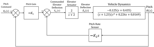
We present a formal analysis of the pitch control system of a UFSS vehicle. The pitch control system is responsible for the uninterrupted operation and functionality of the UFSS vehicle by manipulating different parameters, such as, elevator surface, pitch angle [15]. Fig. 3 depicts its block diagram.
Fig. 3: Pitch Control Model for Unmanned Free-swimming Submersible Vehicle
<details>
<summary>Image 4 Details</summary>
### Visual Description
## Control System Diagram: Vehicle Pitch Control
### Overview
The image is a block diagram representing a closed-loop control system for vehicle pitch control. It shows the relationships between different components, including pitch command, pitch gain, elevator actuator, vehicle dynamics, and pitch rate sensor. The diagram illustrates how feedback is used to regulate the vehicle's pitch.
### Components/Axes
* **Pitch Command:** θe(s) - The desired pitch angle.
* **Pitch Gain:** -K1 - A proportional gain applied to the error signal.
* **Commanded Elevator Deflection:** δe(s) - The desired elevator deflection.
* **Elevator Actuator:** 2/(s+2) - Transfer function of the elevator actuator.
* **Elevator Deflection:** δe(s) - The actual elevator deflection.
* **Vehicle Dynamics:** -0.125(s+0.435) / ((s+1.23)(s^2 + 0.226s + 0.0169)) - Transfer function representing the vehicle's response to elevator deflection.
* **Pitch:** θ(s) - The actual pitch angle of the vehicle.
* **Pitch Rate Sensor:** -K2s - Sensor measuring the pitch rate.
### Detailed Analysis
The system operates as follows:
1. The pitch command θe(s) is compared to the feedback signal from the pitch rate sensor.
2. The error signal is multiplied by the pitch gain -K1.
3. The output of the pitch gain is compared to the feedback signal from the pitch.
4. The resulting signal is the commanded elevator deflection δe(s).
5. The elevator actuator, represented by the transfer function 2/(s+2), converts the commanded deflection into an actual elevator deflection δe(s).
6. The elevator deflection affects the vehicle dynamics, represented by the transfer function -0.125(s+0.435) / ((s+1.23)(s^2 + 0.226s + 0.0169)), resulting in a pitch angle θ(s).
7. The pitch angle is fed back to the initial comparator, and the pitch rate is measured by the pitch rate sensor and fed back to the second comparator, closing the loop.
### Key Observations
* The system uses both pitch angle and pitch rate feedback.
* The vehicle dynamics transfer function is a complex expression involving poles and zeros.
* The elevator actuator is modeled as a first-order system.
### Interpretation
This block diagram represents a closed-loop control system designed to regulate the pitch of a vehicle. The system uses feedback from both the pitch angle and pitch rate to minimize the error between the desired pitch (pitch command) and the actual pitch. The transfer functions for the elevator actuator and vehicle dynamics describe how these components respond to inputs. The gains K1 and K2 are design parameters that can be tuned to achieve desired performance characteristics, such as stability and response time. The negative signs in front of K1 and K2s indicate negative feedback, which is essential for stabilizing the system. The system appears to be designed to maintain a stable pitch angle despite disturbances or changes in the vehicle's environment.
</details>
The dynamics of the UFSS vehicle are represented by its corresponding differential equation, which presents the relationship between the pitch command angle θ e ( t ) and the pitch angle θ ( t ), and is given as follows:
$$\begin{array} { r l r } & { \frac { d ^ { 4 } \theta } { d t ^ { 4 } } + 3 . 4 5 6 \frac { d ^ { 3 } \theta } { d t ^ { 3 } } + ( 3 . 2 0 7 + 0 . 2 5 K _ { 2 } ) \frac { d ^ { 2 } \theta } { d t ^ { 2 } } + ( 0 . 6 1 6 + 0 . 1 0 8 8 K _ { 2 } + 0 . 2 5 K _ { 1 } ) \frac { d \theta } { d t } + } \\ & { ( 0 . 1 0 8 8 K _ { 1 } + 0 . 0 4 1 6 ) = 0 . 2 5 K _ { 1 } \frac { d \theta _ { e } } { d t } + 0 . 1 0 8 8 K _ { 1 } } \end{array} ( 4 )$$
We formalize the above differential equation as follows [18]:
```
Definition 12. 1+ \ K1. inlst ufsv K1 = [Cx(#0.1088) * Cx K1;Cx (#0.25) * Cx K1]
\[Cx(#0.1088) * Cx K1 + Cx(#0.0416);Cx(#0.25) * Cx K1 + Cx(#0.1088) * Cx K2
+ Cx(#0.6106);Cx(#0.25) * Cx K2 + Cx(#3.207);Cx(#3.456);Cx (&1)]
\[ diff eq ufsv inlst ufsv outlst ufsv theta thetae K1 K2 <=>
(\/t. diff eq n order 4 (outlst ufsv K1 K2) theta t =
diff eq n order 1 (inlst ufsv K1) thetae t)
```
where thetae and theta represent the input and the output of the pitch control system and K1 and K2 are the pitch gain and pitch rate sensor gain, respectively. The symbol # is used to represent a decimal number of data type R in HOL Light and is same as symbol & for the integer literal of data type R .
The transfer function of the pitch control of the UFSS vehicle is as follows:
$$\frac { \theta ( s ) } { \theta _ { e } ( s ) } = \frac { 0 . 2 5 K _ { 1 } s + 0 . 1 0 8 8 K _ { 1 } } { s ^ { 4 } + 3 . 4 5 6 s ^ { 3 } + ( 3 . 2 0 7 + 0 . 2 5 K _ { 2 } ) s ^ { 2 } + ( 0 . 6 1 0 6 + 0 . 1 0 8 8 K _ { 2 } + } \quad ( 5 )$$
We verified the above transfer function as the following HOL Light theorem:
```
We verified the above transfer function as the following HOL Light theorem:
Theorem 4. 1 9 thetae theta s K1 K2.
( \forall t . differentiable higher deriv thetae t) ^
laplace exists of higher deriv theta e theta s ^
zero init conditions thetae theta ^
diff eq ufsv inlst ufsv outlst ufsv thetae theta K1 K2 ^
non zero denominator condition theta s
\laplace transform theta s
= laplace transform theta e s
(Cx(#0.25) * Cx K1) * s + Cx(#0.1088) * Cx K1
```
The first two assumptions present the differentiability and the Laplace existence condition of the higher-order derivatives of thetae and theta up to order 1 and 4, respectively. The next assumption provides the zero initial conditions for thetae and theta . The next assumption presents the differential equation specification for the pitch control system of UFSS vehicle. The final assumption models the non-negativity of the denominator of the transfer function presented in the conclusion of the above theorem. We also verified the open loop transfer function θ ( s ) /δ e ( s ), frequency response (open and closed loop) and gain margin, for the UFSS vehicle and the details can be found in [17].
The distinguishing feature of Theorem 4 and the other properties, compared to traditional analysis methods is their generic nature, i.e., all of the variables and functions are universally quantified and can thus be specialized in order to obtain the results for some given values. Moreover, all of the required assumptions are guaranteed to be explicitly mentioned along with the theorems due to the inherent soundness of the theorem proving approach. The high expressiveness of the higher-order logic enables us to model the differential equation and the corresponding transfer function in their true continuous form, whereas, in model checking they are mostly discretized and modeled using a state-transition system, which compromises the accuracy of the analysis.
To facilitate control engineers in using our formalization, we developed an automatic tactic TRANSFER FUN TAC , which automatically verifies the transfer function of the systems up to 20 th -order. This tactic was successfully used for the automatic verification of the transfer functions of the controllers, compensators and the pitch control system of the UFSS vehicle. This automatic verification tactic only requires the differential equation and the transfer function of the
underlying system and automatically verifies the transfer function. Thus, the formal analysis of the UFSS vehicle took only 25 lines of code and about half an hour, thanks to our automatic tactic and the foundational formalization of Section 3.
## 6 Conclusion
This paper presented a higher-order-logic theorem proving based approach for the formal analysis of the dynamical aspects of linear control systems using theorem proving. The main idea behind the proposed framework is to use a formalization of Laplace transform theory in higher-order logic to formally analyze the dynamic aspects of linear control systems. For this purpose, we develop a new formalization of Laplace transform theory, which includes its formal definition and verification of its properties, such as linearity, frequency shifting, differentiation and integration in time domain, time shifting, time scaling, cosine and sinebased modulation and the Laplace transform of an n -order differential equation, which are used for the verification of the transfer function of a generic n -order linear control system. Moreover, the paper also presents the formal verification of some widely used linear control system characteristics, such as frequency response, phase margin and the gain margin, using the verified transfer function, which can be used for the stability analysis of a linear control system. We also formalize the active realization of various controllers, such as PID, PD, PI, P, I, D, and various compensators, such as lag and lead. Finally, we formalize the passive realization of the various compensators, such as lag, lead and lag-lead and verified the corresponding behavioral (differential equation) and the transfer function specifications. To facilitate the usage of these formalizations in analyzing real-world linear control systems, we developed some simplification and automatic verification tactics, in particular the tactic TRANSFER FUN TAC , which automatically verifies the transfer function of any real-world linear control system based on its differential equation. These foundations can be used to analyze a wide range of linear control systems and for illustration purposes, the paper presents the formal analysis of an unmanned free-swimming submersible vehicle.
In future, we plan to link the proposed formalization with Simulink so that the users can provide the system model as a block diagram. This diagram can be used to extract the corresponding transfer function [3], which can in turn be formally verified, almost automatically, to be equivalent to the corresponding block diagram based on the reported formalization and reasoning support.
## Acknowledgements
This work was supported by the National Research Program for Universities grant (number 1543) of Higher Education Commission (HEC), Pakistan.
## References
1. Ahmad, M., Hasan, O.: Formal Verification of Steady-State Errors in UnityFeedback Control Systems. In: Formal Methods for Industrial Critical Systems. pp. 1-15. Springer (2014)
2. Ar´ echiga, N., Loos, S.M., Platzer, A., Krogh, B.H.: Using Theorem Provers to Guarantee Closed-loop System Properties. In: American Control Conference (ACC), 2012. pp. 3573-3580. IEEE (2012)
3. Babuska, R., Stramigioli, S.: Matlab and Simulink for Modeling and Control. Delft University of Technology (1999)
4. Beerends, R.J., Morsche, H.G., Van den Berg, J.C., Van de Vrie, E.M.: Fourier and Laplace Transforms. Cambridge University Press, Cambridge (2003)
5. Beillahi, S.M., Siddique, U., Tahar, S.: Formal Analysis of Power Electronic Systems. In: Formal Engineering Methods. pp. 270-286. Springer (2015)
6. Boulton, R.J., Hardy, R., Martin, U.: A Hoare Logic for Single-input Single-output Continuous-time Control Systems. In: International Workshop on Hybrid Systems: Computation and Control. pp. 113-125. Springer (2003)
7. Ghosh, S.: Control Systems, vol. 1000. Pearson Education (2010)
8. Harrison, J.: HOL Light: A Tutorial Introduction. In: Formal Methods in Computer-Aided Design. LNCS, vol. 1166, pp. 265-269. Springer (1996)
9. Harrison, J.: The HOL Light Theory of Euclidean Space. Journal of Automated Reasoning 50(2), 173-190 (2013)
10. Hasan, O., Ahmad, M.: Formal Analysis of Steady State Errors in Feedback Control Systems using HOL-Light. In: Design, Automation and Test in Europe. pp. 14231426 (2013)
11. Hasan, O., Tahar, S.: Formal verification methods. Encyclopedia of Information Science and Technology, IGI Global Pub pp. 7162-7170 (2015)
12. Johnson, M.E.: Model Checking Safety Properties of Servo-loop Control Systems. In: Dependable Systems and Networks. pp. 45-50. IEEE (2002)
13. Kondo, H., Ura, T.: Navigation of an AUV for Investigation of Underwater Structures. Control Engineering Practice 12(12), 1551-1559 (2004)
14. Lutovac, M., Toˇ si´ c, D.: Symbolic Analysis and Design of Control Systems using Mathematica. International Journal of Control 79(11), 1368-1381 (2006)
15. Nise, N.S.: Control Systems Engineering. John Wiley & Sons (2007)
16. Ogata, K., Yang, Y.: Modern Control Engineering (1970)
17. Rashid, A.: Formal Analysis of Linear Control Systems using Theorem Proving. http://save.seecs.nust.edu.pk/projects/falcstp (2017)
18. Rashid, A., Hasan, O.: On the Formalization of Fourier Transform in Higher-order Logic. In: International Conference on Interactive Theorem Proving. LNCS, vol. 9807, pp. 483-490. Springer (2016)
19. Rashid, A., Hasan, O.: Formalization of Transform Methods using HOL Light. In: Conference on Intelligent Computer Mathematics. LNAI, vol. 10383, pp. 319-332. Springer (2017)
20. Taqdees, S.H., Hasan, O.: Formalization of Laplace Transform Using the Multivariable Calculus Theory of HOL-Light. In: Logic for Programming, Artificial Intelligence, and Reasoning. pp. 744-758. Springer (2013)
21. Taqdees, S.H., Hasan, O.: Formally Verifying Transfer Functions of Linear Analog Circuits. IEEE Design & Test, http://save.seecs.nust.edu.pk/pubs/2017/ DTnA\_2017.pdf (2017)
22. Tiwari, A., Khanna, G.: Series of Abstractions for Hybrid Automata. In: Hybrid Systems: Computation and Control. pp. 465-478. Springer (2002)
23. Wernli, R.L.: Low Cost UUV's for Military Applications: Is the Technology Ready? In: Pacific Congress on Marine Science and Technology (2001)
24. Willcox, S., Vaganay, J., Grieve, R., Rish, J.: The Bluefin BPAUV: An Organic Widearea Bottom Mapping and Mine-hunting Vehicle. Unmanned Untethered Submersible Technology (2001)