## Human in the Loop: Interactive Passive Automata Learning via Evidence-Driven State-Merging Algorithms
Christian A. Hammerschmidt 1 Radu State 1 Sicco Verwer 2
## Abstract
We present an interactive version of an evidencedriven state-merging (EDSM) algorithm for learning variants of finite state automata. Learning these automata often amounts to recovering or reverse engineering the model generating the data despite noisy, incomplete, or imperfectly sampled data sources rather than optimizing a purely numeric target function.
Domain expertise and human knowledge about the target domain can guide this process, and typically is captured in parameter settings. Often, domain expertise is subconscious and not expressed explicitly. Directly interacting with the learning algorithm makes it easier to utilize this knowledge effectively.
## 1. Introduction
Automata, and finite state machines in particular, have long been a formal model used in computer science to designing software and analyzing computer systems themselves (Lee & Yannakakis, 1996). Our knowledge about automata models comes from different source: Firstly, we have studied formal systems in detail and understand them as algebraic systems we can pose decision problems about. Secondly, we have experience lots experience applying them as a model language.
In learning, these tasks are done inversely to recover, reverse-engineer, or understand an unknown data source, typically a communication protocol or software controller. The automata models themselves are also seen as suitable to gain epistemic insight into the system of interest (Hammerschmidt et al., 2016; Vaandrager, 2017) for humans beyond learning models that minimize a given error function, or are used in model checkers for formal analysis.
1 University of Luxembourg 2 Delft Technical University. Correspondence to: Christian A. Hammerschmidt < christian.hammerschmidt@uni.lu > .
Presented at the Human in the Loop workshop at the 34 th International Conference on Machine Learning , Sydney, Australia, 2017. Copyright 2017 by the author(s).
And while we understand the theory of learning automata fairly well, e.g. via learnability results and convergence guarantees, there is a disconnect between the theory of learning algorithms on one side, and domain experts using automata as a modeling language on the other side. How can we bring the two sides together? We propose an interactive version of a learning algorithm with immediate graphical output at each step. This process brings reverse engineering closer to an iterative design process while guiding the process using state-of-the-art heuristics and algorithms. In Section 2, we briefly introduce finite state machines as automata models and outline learning approaches. In 3, we outline our algorithm and provide a small example outlining how our modification is useful. We conclude in Section 4 with an outlook and future work.
## 2. Preliminaries
## 2.1. Automata Models and Finite Automata
The models we consider are variants of deterministic finite state automata, or finite state machines. We provide a conceptual introduction here, and refer to literature for a thorough introduction (Hopcroft et al., 2013). An automaton consists of a set of states, connected by transitions labeled over an alphabet. There is a special start-state where all computations begin, and and a set of final states where computation ends. It is said to accept a word (string) over the alphabet in a computation if there exists a path of transitions from a predefined start state to one of the predefined final states, using transitions labeled with the letters of the word. Automata are called deterministic when there exists exactly one such path for every possible string. Probabilistic automata include probability values on transitions and compute word probabilities using the product of these values along a path, similar to hidden Markov models, rather than having final states. A Mealy machine is a deterministic finite automata that produces an output at each step.
## 2.2. Learning Approaches
Learning automata models, and in particular finite state machines, has long been of interest in the field of grammar induction. While the problem can be solved exactly
(see (Heule & Verwer, 2012)), it is NP-complete. There are two main classes of learning approaches: active learning and passive learning approaches.
In an active setting, the active learner is given the opportunity to interact with an oracle (or teacher) to ask questions about her current hypothesis of the model. Depending on the type of query and answers given by the oracle, different learnability results and algorithms can be obtained (Heinz & Sempere, 2016). The L ∗ algorithm is a successful active learner (Angluin, 1987).
In contrast, the learner in a passive setting has no oracle to interact with. Rather, he is given a fixed set of training data to learn from. In learning stochastic automata, methods based on the methods of moments as well as spectral learning algorithms have been studied (Balle et al., 2014). In Dupont et al. (2008), the authors combine active and passive approaches by asking a user membership queries during a state-merging process.
State-merging algorithms have been very successful in learning probabilistic as well as non-probabilistic automata, and trace back to Oncina & Garcia (1992). Recent state-of-the-art algorithms base on insights from Lang (1998); Verwer et al. (2014). We explain the generic algorithm and our modification in the next section.
## 3. State-Merging and Interactive State-Merging
The starting point for state-merging algorithms is the construction of a tree-shaped automaton from a set of words, the input sample. This initial automaton is called augmented prefix tree acceptor (APTA). It contains all sequences from the input sample, with each sequence element as a directed labeled transition, and states are added to the beginning, end, and between each symbol of the sequence. Two samples share a path in the tree if they share a prefix. The state-merging algorithm reduces the size of the automaton iteratively by merging pairs of states in the model, and forcing the result to be deterministic. The choice of the pairs, and the evaluation of a merge is made heuristically: Each possible merge is evaluated and scored, and the highest scoring merge is executed. This process is repeated and stops if no merges with high scores are possible. These merges generalize the model beyond the samples from the training set: the starting prefix tree is already an acyclic finite automaton. It has a finite set of computations, accepting all words from the training set. Merges can make the resulting automaton cyclic. Automata with cycles accept an infinite set of words. State-merging algorithms generalize by identifying repetitive patterns in the input sample and creating appropriate cycles via merges. Intuitively, the heuristic tries to accomplish this generaliza- tion by identifying pairs of states that have similar future behaviors. In a probabilistic setting, this similarity might be measured by similarity of the empirical probability distributions over the outgoing transition labels. In grammar inference, heuristics rely on occurrence information and the identity of symbols, or use global model selection criteria to calculate merge scores. Finally, the state-merging process as well as the heuristic are controlled by a number of parameters. The general outline of the algorithm is the same as in Algorithm 1, although the user prompt needs to be replaced with execution of the highest scoring merge.
## 3.1. An Interactive Algorithm
Algorithm 1 shows the modified interactive algorithm: Instead of automatically executing the best merge, the graphical visualization of the current model is displayed and the list of possible merges is displayed. The user can choose which of the possible merges to execute by typing its number in the sorted list of possible merges, to backtrack by one step using UNDO , to restart using RESTART , or to automatically execute the next n best merges using LEAP n . Moreover, she can change some global parameter of the algorithm using SET param and see the impact on the proposed merges. Lastly, she can add additional consistency constraints or force merges using the INSERT and FORCE commands. The order of the proposed merges follows the machine learning heuristic. Choosing the first/top merge prosed will lead to the same solution as a single batch-run of the algorithm. The source code for our C++ implementation (as part of out flexfringe tool (Verwer & Hammerschmidt, 2017)) is available in our repository 1 .
In our implementation, the algorithm keeps a stack of executed merges and a list of currently possible merges to store the current state of the algorithm. Based on these data structures, the user has full control over the state-merging process. Additionally, we output the visualization for the last two steps for visual inspection.
## 3.2. Example Use Case
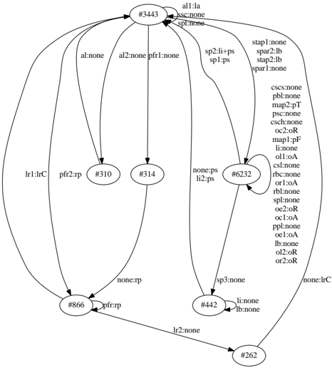
We illustrate the benefits of the interactive mode in a small example: The task is to recover the Mealy machine in Figure 1 from traces sampled from it. 2
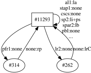
Running an Mealy machine heuristic on 1000 sequences sampled from the model in batch mode yields a wrong
1 https://bitbucket.org/chrshmmmr/dfasat/ src/?at=development
2 For the batch version of our algorithm, this example is provided in an Jupyter notebook environment, see http:// automatonlearning.net/2016/11/04/a-passiveautomata-learning-tutorial-with-dfasat/
Figure 1. The original and fully recovered model of our example use case. State #3443 is the start state. The transitions are annotated with input:output symbols.
<details>
<summary>Image 1 Details</summary>
### Visual Description
## Directed Graph: System Flow Diagram
### Overview
The image displays a directed graph, also known as a state diagram or flowchart, consisting of seven distinct nodes (represented as ellipses with numerical labels) and numerous directed edges connecting them. Each edge is labeled with a colon-separated string, indicating a transition, a relationship, or a condition between nodes. The graph illustrates a complex system with multiple pathways, branching logic, and self-loops, suggesting various states and transitions within a process or system architecture.
### Components/Axes
The diagram is composed solely of nodes and directed edges; it does not feature traditional axes, legends, or scales typically found in charts. All information is embedded within the node and edge labels.
**Nodes (Ellipses with numerical labels):**
* **#3443**: Positioned at the top-center of the diagram. This node appears to be a primary source or initial state, with multiple outgoing edges.
* **#310**: Positioned mid-left, directly below #3443.
* **#314**: Positioned mid-center, directly below #3443.
* **#6232**: Positioned mid-right, directly below #3443. This node is notable for having a large number of self-loops and associated labels.
* **#866**: Positioned at the bottom-left of the diagram.
* **#442**: Positioned at the bottom-center-right of the diagram.
* **#262**: Positioned at the bottom-right of the diagram. This node appears to be a terminal state, as it has no outgoing edges.
**Edges (Directed lines with textual labels):**
Each edge connects a source node to a destination node, with an arrow indicating the direction of flow. Each edge is annotated with a label, typically in the format `[identifier]:[value]` or `[identifier]:[identifier]+[identifier]`. These labels describe the nature of the transition or the condition under which it occurs.
### Detailed Analysis
**Node #3443 (Top-center):**
* **Self-loops (edges originating and terminating at #3443):**
* An edge loops back to #3443 with the label: `all:la`
* An edge loops back to #3443 with the label: `ssc:none`
* An edge loops back to #3443 with the label: `spl:none`
* **Outgoing Edges:**
* To #310 (down-left): `al:none`
* To #314 (down-center): `al2:none`
* To #314 (down-center): `pfr1:none`
* To #6232 (down-right): `sp2:li+ps`
* To #6232 (down-right): `sp1:ps`
* To #866 (long curved path down-left): `lr1:lrC`
* To #442 (long curved path down-right): `none:ps`
* To #442 (long curved path down-right): `li2:ps`
* To #262 (very long curved path down-right): `none:lrC`
**Node #310 (Mid-left):**
* **Incoming Edges:**
* From #3443: `al:none`
* **Outgoing Edges:**
* To #866 (down-left): `pfr2:rp`
**Node #314 (Mid-center):**
* **Incoming Edges:**
* From #3443: `al2:none`
* From #3443: `pfr1:none`
* **Outgoing Edges:**
* To #866 (down-left): `none:rp`
**Node #6232 (Mid-right):
* **Incoming Edges:**
* From #3443: `sp2:li+ps`
* From #3443: `sp1:ps`
* **Self-loops (edges originating and terminating at #6232):**
* An edge loops back to #6232 with the label: `stap1:none`
* An edge loops back to #6232 with the label: `spar2:lb`
* An edge loops back to #6232 with the label: `stap2:lb`
* An edge loops back to #6232 with the label: `spar1:none`
* A large block of text labels a self-loop to #6232, containing multiple colon-separated entries:
`cscs:none`
`pbl:none`
`map2:pT`
`psc:none`
`csch:none`
`oc2:oR`
`map1:pF`
`li:none`
`ol1:oA`
`csl:none`
`rbc:none`
`or1:oA`
`rbl:none`
`spl:none`
`oe2:oR`
`oc1:oA`
`ppl:none`
`oe1:oA`
`lb:none`
`ol2:oR`
`or2:oR`
* **Outgoing Edges:**
* To #442 (down-center): `sp3:none`
**Node #866 (Bottom-left):**
* **Incoming Edges:**
* From #3443: `lr1:lrC`
* From #310: `pfr2:rp`
* From #314: `none:rp`
* **Outgoing Edges:**
* To #442 (short curved path right): `pfr:rp`
**Node #442 (Bottom-center-right):**
* **Incoming Edges:**
* From #3443: `none:ps`
* From #3443: `li2:ps`
* From #6232: `sp3:none`
* From #866: `pfr:rp`
* **Self-loops (edges originating and terminating at #442):**
* An edge loops back to #442 with the label: `li:none`
* An edge loops back to #442 with the label: `lb:none`
* **Outgoing Edges:**
* To #262 (down-right): `lr2:none`
**Node #262 (Bottom-right):**
* **Incoming Edges:**
* From #3443: `none:lrC`
* From #442: `lr2:none`
* **Outgoing Edges:**
* No visible outgoing edges.
### Key Observations
* **Node #3443** serves as a highly connected initial or central node, initiating paths to all other nodes in the graph, including direct paths to #310, #314, #6232, #866, #442, and #262. It also has three self-loops.
* **Node #6232** exhibits the most complex internal behavior, indicated by a large number of self-loops and an extensive list of associated labels. This suggests a state with many internal operations, checks, or attributes that can change without necessarily transitioning to a different major node.
* The label `none` is a very common value in the second part of the edge labels (e.g., `al:none`, `ssc:none`, `sp3:none`, `li:none`), suggesting default conditions, null values, or unconditional transitions.
* Other recurring suffixes in edge labels include `la`, `lb`, `ps`, `rp`, `lrC`, `pT`, `oR`, `pF`, `oA`, which likely denote specific types of states, properties, or outcomes within the system.
* **Node #262** functions as a terminal node or a sink, as it has no outgoing edges. This implies it represents a final state, an endpoint, or a conclusion of a process.
* Multiple paths converge on nodes like #866 (from #3443, #310, #314) and #442 (from #3443, #6232, #866), indicating that these states can be reached through various preceding conditions or sequences.
* The label `sp2:li+ps` on an edge from #3443 to #6232 suggests a composite condition or a combination of attributes (`li` and `ps`) for that specific transition.
### Interpretation
This diagram is a representation of a system's behavior, likely a state machine, a process flow, or a dependency graph. Each numerically labeled ellipse (#3443, #310, etc.) represents a distinct state, a component, a module, or a stage within the system. The numerical labels are unique identifiers for these entities.
The directed edges signify transitions between these states or relationships between components. The labels on these edges provide critical context for understanding these transitions. For example, `al:none` might indicate an "action 'al' occurring without a specific parameter or condition," while `pfr2:rp` could mean "process 'pfr2' results in state 'rp'." The frequent appearance of `none` suggests either default transitions, the absence of a specific value, or conditions that are always met.
**Node #3443** appears to be an initial or central control state, from which various sub-processes or system branches originate. Its self-loops might represent internal initialization routines or minor state adjustments that don't change its fundamental role.
**Node #6232** is particularly complex, suggesting a state that involves extensive internal processing, validation, or a component with numerous configurable attributes. The detailed list of self-loop labels (e.g., `map2:pT`, `oc2:oR`, `ol1:oA`) could represent various internal functions, data mappings (e.g., `pT` for 'pass True', `pF` for 'pass False'), or output/error conditions (e.g., `oR` for 'output result', `oA` for 'output acknowledge').
**Nodes #310 and #314** act as intermediate steps or parallel sub-processes that diverge from #3443 and eventually lead to #866.
**Node #866** serves as a convergence point, indicating a state that can be reached through different preceding sequences, suggesting a common processing stage or a consolidated outcome.
**Node #442** also receives inputs from multiple sources and has its own self-loops, implying further processing or a stable state before the final transition.
**Node #262** is clearly a terminal state, representing the successful completion of a process, an error state, or a final output. The different paths leading to it (`none:lrC` and `lr2:none`) suggest alternative ways to reach this conclusion.
The specific meaning of the prefixes and suffixes in the labels (e.g., `al`, `pfr`, `sp`, `lr`, `li`, `ps`, `rp`, `la`, `lb`, `lrC`, `pT`, `pF`, `oA`, `oR`) would be domain-specific and crucial for a complete understanding of the system's logic. The `+` operator in `sp2:li+ps` implies a logical AND or concatenation of conditions/attributes for that particular transition. This diagram provides a high-level structural and behavioral overview of a system, highlighting its states, transitions, and the conditions governing them.
</details>
model, depicted in Figure 2 3 . Our state-merging algorithm outputs the following sequence of merges and extends:
m147 m182 m207 m10 m58 m79 m98 m47 m69 m62 m54 m57 m69 m71 m70 m83 m81 m97 m104 m117 m144 m158 m181 m221 m254 m305 m343 m413 m539 m119 x162 m264 m259 m0 m1036 m0 x61 m343 m42 m695 m780
There are two types of operations in the algorithm: merges and extensions. The letter m , e.g. m 147 , indicates operation executed was a merge (e.g. with score of 147 ). The letter x indicates and extension, e.g. x 169 indicates that a blue state occurring 169 times was inconsistent with all red states, and no merge could be executed. It therefore is color red. Better evidence, indicated by higher scores and higher occurrence counts, typically leads to better models. Two merges in the sequence above have an evidence of 0. This indicates that despite the lack of evidence for the inconsistency of the merge, there is also little evidence for the merge to be a good choice. Such merges can lead to over-generalization.
A common strategy to deal with this situation, which can occur e.g. due to the lack of sufficient training data or under-sampling specific paths in the model, is to adjust parameters of the statemerger or the heuristic by setting a lower bound on the required merge score and re-running the batch algorithm to resolve further issues 4 . But this is not the only possible parameter to adjust: Other strategies involve changing the relevancy threshold that ig-
3 To reproduce, run ./flexfringe -heuristic-name mealy -data-name mealy data -sinkson 1 -satdfabound 2000 data/original/traces1000.txt on the data in the repository.
4 To reproduce the model in batch mode, run ./flexfringe -
nore traces with low counts (which often can indicate the presence of noise in the collected data).
In our interactive version, a domain expert can immediately react when a merge with lower score is proposed (even without a visual inspection): She can choose to change the thresholds (commands SET state count or SET symbol count ), but they do not change the proposed merges. The expert can decide to exclude the merge by setting a lower bound ( SET lower bound 10), and possible use to restart and leap back to the position of the merge in question. The resulting model, after executing all following proposed merges is the correct model (as depicted in Figure 1) 5 .
In contrast, running the algorithm in batch mode would have required to re-run the complete algorithm multiple times, and comparing the sequence of merges done without the ability to draw up a list of alternative merges for each step.
Figure 2. State #11293 is the start state. The transitions are annotated with input:output symbols. The . . . indicate 30 more input-output pairs on the transition. The model overgeneralizes by merging states together despite low evidence of similarity.
<details>
<summary>Image 2 Details</summary>
### Visual Description
## Diagram: Directed Graph of Interconnected Nodes
### Overview
The image displays a simple directed graph consisting of three nodes: one central square node and two peripheral oval nodes. Arrows indicate the direction of relationships between these nodes, and each arrow is labeled with specific attributes. The central node also features a self-loop with an associated list of key-value pair attributes.
### Components/Nodes and Edges
**Nodes:**
* **Central Node (Square):** Located in the top-center of the diagram, labeled `#11293`.
* **Bottom-Left Node (Oval):** Located in the bottom-left, labeled `#314`.
* **Bottom-Right Node (Oval):** Located in the bottom-right, labeled `#262`.
**Edges (Directed Arrows) and Labels:**
* **From `#314` to `#11293`:** An arrow pointing from the bottom-left oval node to the top-center square node.
* **Label:** `pfr1:none`
* **From `#11293` to `#314`:** An arrow pointing from the top-center square node to the bottom-left oval node.
* **Label:** `none:rp`
* **From `#262` to `#11293`:** An arrow pointing from the bottom-right oval node to the top-center square node.
* **Label:** `lr2:none`
* **From `#11293` to `#262`:** An arrow pointing from the top-center square node to the bottom-right oval node.
* **Label:** `none:lrC`
* **Self-Loop on `#11293`:** An arrow originating from and terminating at the `#11293` node, curving around its top-right side. This loop is associated with a block of text listing attributes.
**Text Block (Associated with Self-Loop on `#111293`):**
Positioned to the top-right of the `#11293` node and its self-loop, this block lists several key-value pairs, vertically stacked:
* `all:la`
* `stap1:none`
* `cscs:none`
* `sp2:li+ps`
* `spar2:lb`
* `pbl:none`
* `...` (An ellipsis indicating that the list continues beyond what is shown).
### Detailed Analysis
The diagram illustrates a network of three entities, identified by numeric IDs. Node `#11293` acts as a central hub, connected to both `#314` and `#262` with bidirectional relationships.
* **Relationships with `#314`:**
* An incoming connection to `#11293` from `#314` is labeled `pfr1:none`.
* An outgoing connection from `#11293` to `#314` is labeled `none:rp`.
* **Relationships with `#262`:**
* An incoming connection to `#11293` from `#262` is labeled `lr2:none`.
* An outgoing connection from `#11293` to `#262` is labeled `none:lrC`.
* **Internal Attributes of `#11293`:** The self-loop on `#11293` signifies internal processes, states, or attributes. The associated text block provides a list of these attributes:
* `all` has a value of `la`.
* `stap1` has a value of `none`.
* `cscs` has a value of `none`.
* `sp2` has a value of `li+ps`.
* `spar2` has a value of `lb`.
* `pbl` has a value of `none`.
* The `...` indicates that there are more attributes not fully displayed.
### Key Observations
* Node `#11293` is the most central and complex node, exhibiting both external bidirectional connections and internal attributes via a self-loop.
* The labels on the edges and some attributes in the self-loop list frequently use the value `none`, suggesting either a default state, an absence of a specific property, or a placeholder.
* The labels `pfr1`, `rp`, `lr2`, `lrC` for the edges, and `all`, `stap1`, `cscs`, `sp2`, `spar2`, `pbl` for the internal attributes, appear to be domain-specific identifiers.
* The numeric node labels (`#11293`, `#314`, `#262`) are likely unique identifiers for entities or components within a larger system.
* The square shape of `#11293` and the oval shape of `#314` and `#262` might denote different types of entities or roles within the system.
### Interpretation
This diagram likely represents a simplified view of a system or process where `#11293` is a critical component, perhaps a central processing unit, a specific state in a finite state machine, or a core service. Nodes `#314` and `#262` could represent other modules, sub-processes, or external dependencies that interact with `#11293`.
The bidirectional arrows indicate a mutual dependency or communication flow between `#11293` and the other two nodes. For instance, `#314` might send a `pfr1:none` signal to `#11293`, which in turn responds with a `none:rp` signal to `#314`. The specific meaning of `none` in these labels would depend on the context of the system being modeled; it could mean "no specific value," "default," or "not applicable."
The self-loop on `#11293` with its associated attributes describes the internal state or configuration of `#11293`. Attributes like `all:la` and `sp2:li+ps` suggest specific internal parameters or capabilities, while `stap1:none`, `cscs:none`, and `pbl:none` might indicate disabled features, default settings, or the absence of certain sub-components. The ellipsis implies that the full internal state is more complex than what is shown, suggesting a detailed configuration or status report for `#11293`.
Overall, the diagram provides a structural and relational overview, highlighting the central role of `#11293` and its interactions, along with a glimpse into its internal characteristics. To fully understand the diagram, the specific domain and meaning of the labels would be required.
</details>
## 4. Conclusion & Future Work
Our experience indicates that a hybrid mode between manual and fully automatic decision is most useful: Especially in cases of large training files (and therefore large initial models which are hard to use visually), automating all decisions until a specific criterion is met (e.g. the best proposed score is below a given threshold, or n merges are executed) takes some burden off the human domain expert while still allowing intervention when necessary. By following the suggestions of the heuristic, the expert can retain learnability guarantees from batch learning algorithms. We have not yet conducted a (formal) analysis to quantify the benefits of interactivity in terms of convergence speed. In Lambeau et al. (2008), the authors experimentally showcase the positive effect of mandatory merge constraints. Similar information, and thus benefits, are provided by the interaction proposed here. Domain expert can implicitly act as a teacher or oracle active learning, bringing together elements from both active and passive learning approaches to automata.
heuristic-name mealy -data-name mealy data -state count 15 symbol count 5 -sinkson 1 -satdfabound 2000 -lowerbound 50 data/original/traces1000.txt on the data in the repository.
5 To reproduce, run ./start.sh interactive-mealy.ini data/original/traces1000.txt from the repository, execute merges until the first m 0 , set lower bound 10 , restart , leap 35 , and execute all merges.
## Acknowledgements
I would like to thank my collages for the valuable discussions and the feedback.
/negationslash
```
```
## References
- Angluin, Dana. Learning regular sets from queries and counterexamples. Information and computation , 75(2):87-106, 1987.
- Balle, Borja, Carreras, Xavier, Luque, Franco M., and Quattoni, Ariadna. Spectral learning of weighted automata: A forwardbackward perspective. Machine Learning , 96(1-2):33-63, July 2014. ISSN 0885-6125, 1573-0565. doi: 10.1007/s10994-0135416-x.
- Dupont, Pierre, Lambeau, Bernard, Damas, Christophe, and Lamsweerde, Axel van. THE QSM ALGORITHM AND ITS
- APPLICATION TO SOFTWARE BEHAVIOR MODEL INDUCTION. Applied Artificial Intelligence , 22(1-2):77-115, February 2008. ISSN 0883-9514, 1087-6545. doi: 10.1080/ 08839510701853200.
- Hammerschmidt, Christian Albert, Lin, Qin, Verwer, Sicco, and State, Radu. Interpreting Finite Automata for Sequential Data. arXiv:1611.07100 [cs, stat] , November 2016. arXiv: 1611.07100.
- Heinz, Jeffrey and Sempere, Jos M. Topics in Grammatical Inference . Springer, 2016.
- Heule, Marijn J. H. and Verwer, Sicco. Software model synthesis using satisfiability solvers. Empirical Software Engineering , 18(4):825-856, August 2012. ISSN 1382-3256, 1573-7616. doi: 10.1007/s10664-012-9222-z.
- Hopcroft, John E., Motwani, Rajeev, and Ullman, Jeffrey D. Introduction to Automata Theory, Languages, and Computation . Pearson, Harlow, Essex, pearson new international edition edition, November 2013. ISBN 978-1-292-03905-3.
- Lambeau, Bernard, Damas, Christophe, and Dupont, Pierre. State-merging DFA induction algorithms with mandatory merge constraints. Grammatical Inference: Algorithms and Applications , pp. 139-153, 2008.
Lang, K. Evidence driven state merging with search. 1998.
- Lee, D. and Yannakakis, M. Principles and methods of testing finite state machines-a survey. Proceedings of the IEEE , 84(8): 1090-1123, August 1996. ISSN 0018-9219. doi: 10.1109/5. 533956.
- Oncina, Jose and Garcia, Pedro. Identifying Regular Languages In Polynomial Time. In Advances in ... , pp. 99-108. World Scientific, 1992.
- Vaandrager, Frits. Model Learning. Commun. ACM , 60(2):86-95, January 2017. ISSN 0001-0782. doi: 10.1145/2967606.
- Verwer, Sicco, Eyraud, Rmi, and De La Higuera, Colin. PAutomaC: a probabilistic automata and hidden Markov models learning competition. Machine learning , 96(1-2):129-154, 2014.
- Verwer, Sicco E. and Hammerschmidt, Christian A. flexfringe: A Passive Automaton Learning Package. September 2017.