1711.00455v3

## A Unified View of Piecewise Linear Neural Network Verification Rudy Bunel University of Oxford ## Ilker Turkaslan rudy@robots.ox.ac.uk University of Oxford ilker.turkaslan@lmh.ox.ac.uk Pushmeet Kohli Deepmind pushmeet@google.com Philip H.S. Torr University of Oxford philip.torr@eng.ox.ac.uk M. Pawan Kumar University of Oxford Alan Turing Institute pawan@robots.ox.ac.uk ## Abstract The success of Deep Learning and its potential use in many safety-critical applications has motivated research on formal verification of Neural Network (NN) models. Despite the reputation of learned NN models to behave as black boxes and the theoretical hardness of proving their properties, researchers have been successful in verifying some classes of models by exploiting their piecewise linear structure and taking insights from formal methods such as Satisifiability Modulo Theory. These methods are however still far from scaling to realistic neural networks. To facilitate progress on this crucial area, we make two key contributions. First, we present a unified framework that encompasses previous methods. This analysis results in the identification of new methods that combine the strengths of multiple existing approaches, accomplishing a speedup of two orders of magnitude compared to the previous state of the art. Second, we propose a new data set of benchmarks which includes a collection of previously released testcases. We use the benchmark to provide the first experimental comparison of existing algorithms and identify the factors impacting the hardness of verification problems. ## 1 Introduction Despite their success in a wide variety of applications, Deep Neural Networks have seen limited adoption in safety-critical settings. The main explanation for this lies in their reputation for being black-boxes whose behaviour can not be predicted. Current approaches to evaluate trained models mostly rely on testing using held-out data sets. However, as Edsger W. Dijkstra said [3], 'testing shows the presence, not the absence of bugs'. If deep learning models are to be deployed to applications such as autonomous driving cars, we need to be able to verify safety-critical behaviours. To this end, some researchers have tried to use formal methods. To the best of our knowledge, Zakrzewski [21] was the first to propose a method to verify simple, one hidden layer neural networks. However, only recently were researchers able to work with non-trivial models by taking advantage of the structure of ReLU-based networks [5, 11]. Even then, these works are not scalable to the large networks encountered in most real world problems. This paper advances the field of NN verification by making the following key contributions: 1. We reframe state of the art verification methods as special cases of Branch-and-Bound optimization, which provides us with a unified framework to compare them. 2. We gather a data set of test cases based on the existing literature and extend it with new benchmarks. We provide the first experimental comparison of verification methods. 3. Based on this framework, we identify algorithmic improvements in the verification process, specifically in the way bounds are computed, the type of branching that are considered, as Preprint. Work in progress. well as the strategies guiding the branching. Compared to the previous state of the art, these improvements lead to speed-up of almost two orders of magnitudes . Section 2 and 3 give the specification of the problem and formalise the verification process. Section 4 presents our unified framework, showing that previous methods are special cases and highlighting potential improvements. Section 5 presents our experimental setup and Section 6 analyses the results. ## 2 Problem specification We now specify the problem of formal verification of neural networks. Given a network that implements a function ˆ x n = f ( x 0 ) , a bounded input domain C and a property P , we want to prove $$x _ { 0 } \in \mathcal { C } , \quad \hat { x } _ { n } = f ( x _ { 0 } ) \implies P ( \hat { x } _ { n } ) . \quad ( 1 )$$ For example, the property of robustness to adversarial examples in L ∞ norm around a training sample a with label y a would be encoded by using C /defines { x 0 | ‖ x 0 -a ‖ ∞ ≤ /epsilon1 } and P ( ˆ x n ) = { ∀ y ˆ x n [ y a ] ≥ ˆ x n [ y ] } . In this paper, we are going to focus on Piecewise-Linear Neural Networks (PL-NN), that is, networks for which we can decompose C into a set of polyhedra C i such that C = ∪ i C i , and the restriction of f to C i is a linear function for each i . While this prevents us from including networks that use activation functions such as sigmoid or tanh, PL-NNs allow the use of linear transformations such as fully-connected or convolutional layers, pooling units such as MaxPooling and activation functions such as ReLUs. In other words, PL-NNs represent the majority of networks used in practice. Operations such as Batch-Normalization or Dropout also preserve piecewise linearity at test-time. The properties that we are going to consider are Boolean formulas over linear inequalities. In our robustness to adversarial example above, the property is a conjunction of linear inequalities, each of which constrains the output of the original label to be greater than the output of another label. The scope of this paper does not include approaches relying on additional assumptions such as twice differentiability of the network [8, 21], limitation of the activation to binary values [5, 16] or restriction to a single linear domain [2]. Since they do not provide formal guarantees, we also don't include approximate approaches relying on a limited set of perturbation [10] or on over-approximation methods that potentially lead to undecidable properties [17, 20]. ## 3 Verification Formalism ## 3.1 Verification as a Satisfiability problem The methods we involve in our comparison all leverage the piecewise-linear structure of PL-NN to make the problem more tractable. They all follow the same general principle: given a property to prove, they attempt to discover a counterexample that would make the property false. This is accomplished by defining a set of variables corresponding to the inputs, hidden units and output of the network, and the set of constraints that a counterexample would satisfy. To help design a unified framework, we reduce all instances of verification problems to a canonical representation. Specifically, the whole satisfiability problem will be transformed into a global optimization problem where the decision will be obtained by checking the sign of the minimum. If the property to verify is a simple inequality P ( ˆ x n ) /defines c T ˆ x n ≥ b , it is sufficient to add to the network a final fully connected layer with one output, with weight of c and a bias of -b . If the global minimum of this network is positive, it indicates that for all ˆ x n the original network can output, we have c T ˆ x n -b ≥ 0 = ⇒ c T ˆ x n ≥ b , and as a consequence the property is True. On the other hand, if the global minimum is negative, then the minimizer provides a counter-example. The supplementary material shows that OR and AND clauses in the property can similarly be expressed as additional layers, using MaxPooling units. We can formulate any Boolean formula over linear inequalities on the output of the network as a sequence of additional linear and max-pooling layers. The verification problem will be reduced to the problem of finding whether the scalar output of the potentially modified network can reach a negative value. Assuming the network only contains ReLU activations between each layer, the satisfiability problem to find a counterexample can be expressed as: $$l _ { 0 } \leq x _ { 0 } \leq u _ { 0 } \quad ( 2 a ) \quad \hat { x } _ { i + 1 } = W _ { i + 1 } x _ { i } + b _ { i + 1 } \quad \forall i \in \{ 0 , \, n - 1 \} \quad ( 2 c )$$ x ˆ n ≤ $$\begin{array} { r l r } { \leq 0 } & ( 2 b ) } & x _ { i } = \max \left ( \hat { x } _ { i } , 0 \right ) } & \forall i \in \{ 1 , \, n - 1 \} . } & ( 2 d ) } \end{array}$$ Eq. (10a) represents the constraints on the input and Eq. (10h) on the neural network output. Eq. (10b) encodes the linear layers of the network and Eq. (2d) the ReLU activation functions. If an assignment to all the values can be found, this represents a counterexample. If this problem is unsatisfiable, no counterexample can exist, implying that the property is True. We emphasise that we are required to prove that no counter-examples can exist, and not simply that none could be found. While for clarity of explanation, we have limited ourselves to the specific case where only ReLU activation functions are used, this is not restrictive. The supplementary material contains a section detailing how each method specifically handles MaxPooling units, as well as how to convert any MaxPooling operation into a combination of linear layers and ReLU activation functions. The problem described in (2) is still a hard problem. The addition of the ReLU non-linearities (2d) transforms a problem that would have been solvable by simple Linear Programming into an NP-hard problem [11]. Converting a verification problem into this canonical representation does not make its resolution simpler but it does provide a formalism advantage. Specifically, it allows us to prove complex properties, containing several OR clauses, with a single procedure rather than having to decompose the desired property into separate queries as was done in previous work [11]. Operationally, a valid strategy is to impose the constraints (10a) to (2d) and minimise the value of ˆ x n . Finding the exact global minimum is not necessary for verification. However, it provides a measure of satisfiability or unsatisfiability. If the value of the global minimum is positive, it will correspond to the margin by which the property is satisfied. ## 3.2 Mixed Integer Programming formulation A possible way to eliminate the non-linearities is to encode them with the help of binary variables, transforming the PL-NN verification problem (2) into a Mixed Integer Linear Program (MIP). This can be done with the use of 'big-M' encoding. The following encoding is from Tjeng & Tedrake [19]. Assuming we have access to lower and upper bounds on the values that can be taken by the coordinates of ˆ x i , which we denote l i and u i , we can replace the non-linearities: $$\begin{array} { r l r } { x _ { i } = \max \left ( \hat { x } _ { i } , 0 \right ) } & { \Rightarrow } & { \delta _ { i } \in \{ 0 , 1 \} ^ { h _ { i } } , \, x _ { i } \geq 0 , \quad x _ { i } \leq u _ { i } \cdot \delta _ { i } \quad ( 3 a ) } \end{array}$$ $$x _ { i } \geq \hat { x } _ { i } , \quad x _ { i } \leq \hat { x } _ { i } - l _ { i } \cdot ( 1 - \delta _ { i } ) \quad ( 3 b )$$ It is easy to verify that δ i [ j ] = 0 ⇔ x i [ j ] = 0 (replacing δ i [ j ] in Eq. (21a)) and δ i [ j ] = 1 ⇔ x i [ j ] = ˆ x i [ j ] (replacing δ i [ j ] in Eq. (21b)). By taking advantage of the feed-forward structure of the neural network, lower and upper bounds l i and u i can be obtained by applying interval arithmetic [9] to propagate the bounds on the inputs, one layer at a time. Thanks to this specific feed-forward structure of the problem, the generic, non-linear, non-convex problem has been rewritten into an MIP. Optimization of MIP is well studied and highly efficient off-the-shelf solvers exist. As solving them is NP-hard, performance is going to be dependent on the quality of both the solver used and the encoding. We now ask the following question: how much efficiency can be gained by using a bespoke solver rather than a generic one? In order to answer this, we present specialised solvers for the PLNN verification task. ## 4 Branch-and-Bound for Verification As described in Section 3.1, the verification problem can be rephrased as a global optimization problem. Algorithms such as Stochastic Gradient Descent are not appropriate as they have no way of guaranteeing whether or not a minima is global. In this section, we present an approach to estimate the global minimum, based on the Branch and Bound paradigm and show that several published methods, introduced as examples of Satisfiability Modulo Theories, fit this framework. Algorithm 1 describes its generic form. The input domain is repeatedly split into sub-domains (line 7), over which lower and upper bounds of the minimum are computed (lines 9-10). The best upperbound found so far serves as a candidate for the global minimum. Any domain whose lower bound is greater than the current global upper bound can be pruned away as it cannot contain the global minimum (line 13, lines 15-17). By iteratively splitting the domains, it is possible to compute tighter lower bounds. We keep track of the global lower bound on the minimum by taking the minimum over the lower bounds of all sub-domains (line 19). When the global upper bound and the global lower bound differ by less than a small scalar /epsilon1 (line 5), we consider that we have converged. Algorithm 1 shows how to optimise and obtain the global minimum. If all that we are interested in is the satisfiability problem, the procedure can be simplified by initialising the global upper bound with 0 (in line 2). Any subdomain with a lower bound greater than 0 (and therefore not eligible to contain a counterexample) will be pruned out (by line 15). The computation of the lower bound can therefore be replaced by the feasibility problem (or its relaxation) imposing the constraint that the output is below zero without changing the algorithm. If it is feasible, there might still be a counterexample and further branching is necessary. If it is infeasible, the subdomain can be pruned out. In addition, if any upper bound improving on 0 is found on a subdomain (line 11), it is possible to stop the algorithm as this already indicates the presence of a counterexample. ## Algorithm 1 Branch and Bound ``` Algorithm 1 Branch and Bound <section_header_level_1><loc_69><loc_45><loc_431><loc_75>1: function BAB(net, domain, ϵ)</section_header_level_1> <text><loc_68><loc_76><loc_432><loc_105>2: global_ub ← inf</text> <text><loc_68><loc_106><loc_433><loc_125>3: global_lb ← -inf</text> <text><loc_69><loc_126><loc_431><loc_145>4: doms ← [(global_lb, domain)]</text> <text><loc_69><loc_146><loc_432><loc_165>5: while global_ub - global_lb > ϵ do</text> <text><loc_68><loc_166><loc_431><loc_185>6: (_, dom) <- pick_out(doms)</text> <text><loc_69><loc_186><loc_432><loc_205>7: [subdom_1,..., subdom_s] ← split(dom)</text> <text><loc_68><loc_206><loc_431><loc_225>8: for i = 1 ... s do</text> <text><loc_69><loc_226><loc_432><loc_245>9: dom_ub <- compute_UB(net, subdom_i)</text> <text><loc_68><loc_246><loc_431><loc_265>10: dom_lb <- compute_LB(net, subdom_i)</text> <text><loc_69><loc_266><loc_432><loc_285>11: if dom_ub < global_ub then</text> <text><loc_68><loc_286><loc_431><loc_305>12: global_ub ← dom_ub</text> <text><loc_68><loc_306><loc_433><loc_325>13: prune_domains(doms, global_ub)</text> <text><loc_69><loc_326><loc_432><loc_345>14: end if</text> <text><loc_68><loc_346><loc_431><loc_365>15: if dom_lb < global_ub then</text> <text><loc_68><loc_366><loc_433><loc_385>16: domains.append((dom_lb, subdom_i))</text> <text><loc_69><loc_386><loc_432><loc_405>17: end if</text> <text><loc_68><loc_406><loc_431><loc_425>18: end for</text> <text><loc_68><loc_426><loc_433><loc_445>19: global_lb ← min{lb | (lb, dom) ∈ doms}</text> <text><loc_69><loc_446><loc_432><loc_465>20: end while</text> <text><loc_69><loc_466><loc_431><loc_485>21: return global_ub</text> </doctag> ``` greatly impact the quality of the resulting bounds. Bounding methods , defined by the compute \_ { UB , LB } functions. These procedures estimate respectively upper bounds and lower bounds over the minimum output that the network net can reach over a given input domain. We want the lower bound to be as high as possible, so that this whole domain can be pruned easily. This is usually done by introducing convex relaxations of the problem and minimising them. On the other hand, the computed upper bound should be as small as possible, so as to allow pruning out other regions of the space or discovering counterexamples. As any feasible point corresponds to an upper bound on the minimum, heuristic methods are sufficient. We now demonstrate how some published work in the literature can be understood as special case of the branch-and-bound framework for verification. ## 4.1 Reluplex Katz et al. [11] present a procedure named Reluplex to verify properties of Neural Network containing linear functions and ReLU activation unit, functioning as an SMT solver using the splitting-ondemand framework [1]. The principle of Reluplex is to always maintain an assignment to all of the variables, even if some of the constraints are violated. Starting from an initial assignment, it attempts to fix some violated constraints at each step. It prioritises fixing linear constraints ((10a), (10b), (10h) and some relaxation of (2d)) using a simplex algorithm, even if it leads to violated ReLU constraints. If no solution to this relaxed problem containing only linear constraints exists, the counterexample search is unsatisfiable. Otherwise, either all ReLU are respected, which generates a counterexample, or Reluplex attempts to fix one of the violated ReLU; potentially leading to newly violated linear constraints. This process is not guaranteed to converge, so to make progress, non-linearities that get fixed too often are split into two cases. Two new problems are generated, each corresponding to one of the phases of the ReLU. In the worst setting, the problem will be split completely over all possible combinations of activation patterns, at which point the sub-problems will all be simple LPs. This algorithm can be mapped to the special case of branch-and-bound for satisfiability. The search strategy is handled by the SMT core and to the best of our knowledge does not prioritise any domain. The branching rule is implemented by the ReLU-splitting procedure: when neither the upper bound search, nor the detection of infeasibility are successful, one non-linear constraint over the j -th neu- The description of the verification problem as optimization and the pseudo-code of Algorithm 1 are generic and would apply to verification problems beyond the specific case of PLNN. To obtain a practical algorithm, it is necessary to specify several elements. A search strategy , defined by the pick \_ out function, which chooses the next domain to branch on. Several heuristics are possible, for example those based on the results of previous bound computations. For satisfiable problems or optimization problems, this allows to discover good upper bounds, enabling early pruning. /negationslash A branching rule , defined by the split function, which takes a domain dom and return a partition in subdomain such that ⋃ i subdom \_ i = dom and that ( subdom \_ i ∩ subdom \_ j ) = ∅ , ∀ i = j . This will define the 'shape' of the domains, which impacts the hardness of computing bounds. In addition, choosing the right partition can ron of the i -th layer x i [ j ] = max ( ˆ x i [ j ] , 0 ) is split out into two subdomains: { x i [ j ] = 0 , ˆ x i [ j ] ≤ 0 } and { x i [ j ] = ˆ x i [ j ] , ˆ x i [ j ] ≥ 0 } . This defines the type of subdomains produced. The prioritisation of ReLUs that have been frequently fixed is a heuristic to decide between possible partitions. As Reluplex only deal with satisfiability, the analogue of the lower bound computation is an overapproximation of the satisfiability problem. The bounding method used is a convex relaxation, obtained by dropping some of the constraints. The following relaxation is applied to ReLU units for which the sign of the input is unknown ( l i [ j ] ≤ 0 and u i [ j ] ≥ 0 ). $$x _ { i } = \max \left ( \hat { x } _ { i } , 0 \right ) \quad \Rightarrow \quad x _ { i } \geq \hat { x } _ { i } \quad ( 4 a ) \quad \ x _ { i } \geq 0 \quad ( 4 b ) \quad \ x _ { i } \leq u _ { i } . \quad ( 4 c )$$ If this relaxation is unsatisfiable, this indicates that the subdomain cannot contain any counterexample and can be pruned out. The search for an assignment satisfying all the ReLU constraints by iteratively attempting to correct the violated ReLUs is a heuristic that is equivalent to the search for an upper bound lower than 0: success implies the end of the procedure but no guarantees can be given. ## 4.2 Planet Ehlers [6] also proposed an approach based on SMT. Unlike Reluplex, the proposed tool, named Planet, operates by explicitly attempting to find an assignment to the phase of the non-linearities. Reusing the notation of Section 3.2, it assigns a value of 0 or 1 to each δ i [ j ] variable, verifying at each step the feasibility of the partial assignment so as to prune infeasible partial assignment early. As in Reluplex, the search strategy is not explicitly encoded and simply enumerates all the domains that have not yet been pruned. The branching rule is the same as for Reluplex, as fixing the decision variable δ i [ j ] = 0 is equivalent to choosing { x i [ j ] = 0 , ˆ x i [ j ] ≤ 0 } and fixing δ i [ j ] = 1 is equivalent to { x i [ j ] = ˆ x i [ j ] , ˆ x i [ j ] ≥ 0 } . Note however that Planet does not include any heuristic to prioritise which decision variables should be split over. Planet does not include a mechanism for early termination based on a heuristic search of a feasible point. For satisfiable problems, only when a full complete assignment is identified is a solution returned. In order to detect incoherent assignments, Ehlers [6] introduces a global linear approximation to a neural network, which is used as a bounding method to over-approximate the set of values that each hidden unit can take. In addition to the existing linear constraints ((10a), (10b) and (10h)), the non-linear constraints are approximated by sets of linear constraints representing the non-linearities' convex hull. Specifically, ReLUs with input of unknown sign are replaced by the set of equations: $$\begin{array} { r l } & { x _ { i } = \max ( \hat { x } _ { i } , 0 ) \, \Rightarrow \, x _ { i } \geq \hat { x } _ { i } \quad ( 5 a ) \quad x _ { i } \geq 0 \quad ( 5 b ) \quad x _ { i [ j ] } \leq u _ { i [ j ] } \frac { \hat { x } _ { i [ j ] } - l _ { i [ j ] } } { u _ { i [ j ] } - l _ { i [ j ] } } \quad ( 5 c ) } \\ & { w h o r a n d o p e r r o s p o n d e t h e v a l u o f t h e i t h o o r d i n a t e o f x _ { i [ j ] } . \quad A n i l l u r t r a c t i o n o f t h e f a g i b l e } \end{array}$$ where x i [ j ] corresponds to the value of the j -th coordinate of x i . An illustration of the feasible domain is provided in the supplementary material. Compared with the relaxation of Reluplex (4), the Planet relaxation is tighter. Specifically, Eq. (4a) and (4b) are identical to Eq. (5a) and (5b) but Eq. (5c) implies Eq. (4c). Indeed, given that ˆ x i [ j ] is smaller than u i [ j ] , the fraction multiplying u i [ j ] is necessarily smaller than 1, implying that this provides a tighter bounds on x i [ j ] . To use this approximation to compute better bounds than the ones given by simple interval arithmetic, it is possible to leverage the feed-forward structure of the neural networks and obtain bounds one layer at a time. Having included all the constraints up until the i -th layer, it is possible to optimize over the resulting linear program and obtain bounds for all the units of the i -th layer, which in turn will allow us to create the constraints (5) for the next layer. In addition to the pruning obtained by the convex relaxation, both Planet and Reluplex make use of conflict analysis [15] to discover combinations of splits that cannot lead to satisfiable assignments, allowing them to perform further pruning of the domains. ## 4.3 Potential improvements As can be seen, previous approaches to neural network verification have relied on methodologies developed in three communities: optimization, for the creation of upper and lower bounds; verification, especially SMT; and machine learning, especially the feed-forward nature of neural networks for the creation of relaxations. A natural question that arises is 'Can other existing literature from these domains be exploited to further improve neural network verification?' Our unified branch-andbound formulation makes it easy to answer this question. To illustrate its power, we now provide a non-exhaustive list of suggestions to speed-up verification algorithms. Better bounding While the relaxation proposed by Ehlers [6] is tighter than the one used by Reluplex, it can be improved further still. Specifically, after a splitting operation, on a smaller domain, we can refine all the l i , u i bounds, to obtain a tither relaxation. We show the importance of this in the experiments section with the BaB-relusplit method that performs splitting on the activation like Planet but updates its approximation completely at each step. One other possible area of improvement lies in the tightness of the bounds used. Equation (5) is very closely related to the Mixed Integer Formulation of Equation (20). Indeed, it corresponds to level 0 of the Sherali-Adams hierarchy of relaxations [18]. The proof for this statement can be found in the supplementary material. Stronger relaxations could be obtained by exploring higher levels of the hierarchy. This would jointly constrain groups of ReLUs, rather than linearising them independently. Better branching The decision to split on the activation of the ReLU non-linearities made by Planet and Reluplex is intuitive as it provides a clear set of decision variables to fix. However, it ignores another natural branching strategy, namely, splitting the input domain. Indeed, it could be argued that since the function encoded by the neural networks are piecewise linear in their input, this could result in the computation of highly useful upper and lower bounds. To demonstrate this, we propose the novel BaB-input algorithm: a branch-and-bound method that branches over the input features of the network. Based on a domain with input constrained by Eq. (10a), the split function would return two subdomains where bounds would be identical in all dimension except for the dimension with the largest length, denoted i /star . The bounds for each subdomain for dimension i /star are given by l 0[ i /star ] ≤ x 0[ i /star ] ≤ l 0[ i /star ] + u 0[ i /star ] 2 and l 0[ i /star ] + u 0[ i /star ] 2 ≤ x 0[ i /star ] ≤ u 0[ i /star ] . Based on these tighter input bounds, tighter bounds at all layers can be re-evaluated. One of the main advantage of branching over the variables is that all subdomains generated by the BaB algorithm when splitting over the input variables end up only having simple bound constraints over the value that input variable can take. In order to exploit this property to the fullest, we use the highly efficient lower bound computation approach of Kolter & Wong [13]. This approach was initially proposed in the context of robust optimization. However, our unified framework opens the door for its use in verification. Specifically, Kolter & Wong [13] identified an efficient way of computing bounds for the type of problems we encounter, by generating a feasible solution to the dual of the LP generated by the Planet relaxation. While this bound is quite loose compared to the one obtained through actual optimization, they are very fast to evaluate. We propose a smart branching method BaBSB to replace the longest edge heuristic of BaB-input . For all possible splits, we compute fast bounds for each of the resulting subdomain, and execute the split resulting in the highest lower bound. The intuition is that despite their looseness, the fast bounds will still be useful in identifying the promising splits. ## 5 Experimental setup The problem of PL-NN verification has been shown to be NP-complete [11]. Meaningful comparison between approaches therefore needs to be experimental. ## 5.1 Methods The simplest baseline we refer to is BlackBox , a direct encoding of Eq. (2) into the Gurobi solver, which will perform its own relaxation, without taking advantage of the problem's structure. For the SMT based methods, Reluplex and Planet , we use the publicly available versions [7, 12]. Both tools are implemented in C++ and relies on the GLPK library to solve their relaxation. We wrote some software to convert in both directions between the input format of both solvers. We also evaluate the potential of using MIP solvers, based on the formulation of Eq. (20). Due to the lack of availability of open-sourced methods at the time of our experiments, we reimplemented the approach in Python, using the Gurobi MIP solver. We report results for a variant called MIPplanet , which uses bounds derived from Planet's convex relaxation rather than simple interval arithmetic. The MIP is not treated as a simple feasibility problem but is encoded to minimize the output ˆ x n of Equation (10h), with a callback interrupting the optimization as soon as a negative value is found. Additional discussions on encodings of the MIP problem can be found in supplementary materials. In our benchmark, we include the methods derived from our Branch and Bound analysis. Our implementation follows faithfully Algorithm 1, is implemented in Python and uses Gurobi to solve LPs. The pick \_ out strategy consists in prioritising the domain that currently has the smallest lower bound. Upper bounds are generated by randomly sampling points on the considered domain, and we use the convex approximation of Ehlers [6] to obtain lower bounds. 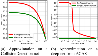As opposed to the approach taken by Ehlers [6] of building a single approximation of the network, we rebuild the approximation and recompute all bounds for each sub-domain. This is motivated by the observation shown in Figure 1 which demonstrate the significant improvements it brings, especially for deeper networks. For split , BaB-input performs branching by splitting the input domain in half along its longest edge and BaBSB does it by splitting the input domain along the dimension improving the global lower bound the most according to the fast bounds of Kolter & Wong [13]. We also include results for the BaB-relusplit variant, where the split method is based on the phase of the non-linearities, similarly to Planet . <details> <summary>Image 1 Details</summary>  ### Visual Description ## Line Graphs: Approximation Performance Comparison ### Overview The image contains two line graphs comparing the performance of two approximation methods ("ReApproximating" and "FixedApproximation") across different relative areas. Graph (a) focuses on lower bound values, while graph (b) examines error scores. Both graphs use logarithmic scales on the x-axis (relative area) and linear scales on the y-axis. ### Components/Axes **Graph (a):** - **Y-axis (Left):** "Lower bound" (32.0 to 36.0, linear scale) - **X-axis:** "Relative area" (10⁻¹² to 10⁰, logarithmic scale) - **Legend:** Top-right corner, labels: - Red line: "ReApproximating" - Green line: "FixedApproximation" **Graph (b):** - **Y-axis (Left):** "Error score" (-10⁵ to 10³, logarithmic scale) - **X-axis:** "Relative area" (10⁻⁶ to 10⁰, logarithmic scale) - **Legend:** Top-right corner, same labels as graph (a) ### Detailed Analysis **Graph (a):** - **ReApproximating (Red):** Starts at 36.0 (x=10⁻¹²), decreases smoothly, and intersects the green line at ~10⁻³ relative area. Ends near 32.5 at x=10⁰. - **FixedApproximation (Green):** Starts at 34.8 (x=10⁻¹²), decreases gradually, and remains below the red line until intersection. Ends near 32.2 at x=10⁰. **Graph (b):** - **ReApproximating (Red):** Starts at 10³ (x=10⁻⁶), drops sharply to -10⁵ at x=10⁻³, then stabilizes near -10⁵. - **FixedApproximation (Green):** Remains constant at -10⁵ across all relative areas. ### Key Observations 1. **Graph (a):** - ReApproximating begins with a higher lower bound but converges with FixedApproximation as relative area increases. - Intersection at ~10⁻³ suggests parity in performance at small relative areas. 2. **Graph (b):** - ReApproximating shows a dramatic error reduction at x=10⁻³, while FixedApproximation maintains a constant low error. - Red line's sharp decline indicates superior error handling at small relative areas. ### Interpretation - **Performance Trade-offs:** - ReApproximating outperforms FixedApproximation at small relative areas (graph b) but starts with a higher lower bound (graph a). - FixedApproximation offers stability but lacks adaptability at extreme scales. - **Practical Implications:** - ReApproximating may be preferable for systems requiring precision at small scales, while FixedApproximation suits scenarios prioritizing consistency. - **Anomalies:** - The sharp drop in graph (b) for ReApproximating at x=10⁻³ suggests a threshold effect, warranting further investigation into its underlying mechanism. 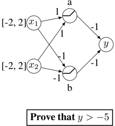</details> ## 5.2 Evaluation Criteria Figure 1: Quality of the linear approximation, depending on the size of the input domain. We plot the value of the lower bound as a function of the area on which it is computed (higher is better). The domains are centered around the global minimum and repeatedly shrunk. Rebuilding completely the linear approximation at each step allows to create tighter lower-bounds thanks to better l i and u i , as opposed to using the same constraints and only changing the bounds on input variables. This effect is even more significant on deeper networks. For each of the data sets, we compare the different methods using the same protocol. We attempt to verify each property with a timeout of two hours, and a maximum allowed memory usage of 20GB, on a single core of a machine with an i7-5930K CPU. We measure the time taken by the solvers to either prove or disprove the property. If the property is false and the search problem is therefore satisfiable, we expect from the solver to exhibit a counterexample. If the returned input is not a valid counterexample, we don't count the property as successfully proven, even if the property is indeed satisfiable. All code and data necessary to replicate our analysis are released. ## 6 Analysis We attempt to perform verification on three data sets of properties and report the comparison results. The dimensions of all the problems can be found in the supplementary material. 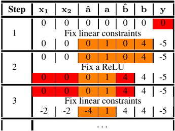The CollisionDetection data set [6] attempts to predict whether two vehicles with parameterized trajectories are going to collide. 500 properties are extracted from problems arising from a binary search to identify the size of the region around training examples in which the prediction of the network does not change. The network used is relatively shallow but due to the process used to generate the properties, some lie extremely close between the decision boundary between SAT and UNSAT. Results presented in Figure 10 therefore highlight the accuracy of methods. The Airborne Collision Avoidance System (ACAS) data set, as released by Katz et al. [11] is a neural network based advisory system recommending horizontal manoeuvres for an aircraft in order to avoid collisions, based on sensor measurements. Each of the five possible manoeuvres is assigned a score by the neural network and the action with the minimum score is chosen. The 188 properties to verify are based on some specification describing various scenarios. Due to the deeper network involved, this data set is useful in highlighting the scalability of the various algorithms. PCAMNIST is a novel data set that we introduce to get a better understanding of what factors influence the performance of various methods. It is generated in a way to give control over different architecture parameters. Details of the dataset construction are given in supplementary materials. We present plots in Figure 4 showing the evolution of runtimes depending on each of the architectural parameters of the networks. 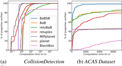Comparative evaluation of verification approaches In Figure 10, on the shallow networks of CollisionDetection , most solvers succeed against all properties in about 10s. In particular, the SMT inspired solvers Planet , Reluplex and the MIP solver are extremely fast. The BlackBox solver doesn't reach 100% accuracy due to producing incorrect counterexamples. Additional analysis can be found about the cause of those errors in the supplementary materials. On the deeper networks of ACAS , in Figure 10b, no errors are observed but most methods timeout on the most challenging testcases. The best baseline is Reluplex , who reaches 79.26% success rate at the two hour timeout, while our best method, BaBSB , already achieves 98.40% with a budget of one hour. To reach Reluplex's success rate, the required runtime is two orders of magnitude smaller. <details> <summary>Image 2 Details</summary>  ### Visual Description ## Line Graphs: Algorithm Performance Comparison ### Overview The image contains two line graphs comparing the performance of various algorithms in verifying properties over computation time. Graph (a) focuses on "CollisionDetection," while graph (b) analyzes the "ACAS Dataset." Both graphs plot computation time (x-axis) against the percentage of properties verified (y-axis). ### Components/Axes - **Graph (a): CollisionDetection** - **X-axis**: Computation time (logarithmic scale, 10⁻¹ to 10³ seconds). - **Y-axis**: % of properties verified (0–100%). - **Legend**: - BaBSB (blue) - BaB (orange) - reluBaB (green) - reluplex (red) - MIPplanet (purple) - planet (brown) - BlackBox (pink) - **Key Features**: - Dotted horizontal line at 100% (y-axis). - Lines start at the origin (0,0) and ascend to varying degrees. - **Graph (b): ACAS Dataset** - **X-axis**: Computation time (linear scale, 0 to 6000 seconds). - **Y-axis**: % of properties verified (0–100%). - **Legend**: Same algorithms as graph (a). - **Key Features**: - Dotted horizontal line at 100% (y-axis). - Lines start at the origin (0,0) and ascend more gradually. ### Detailed Analysis #### Graph (a): CollisionDetection - **BaBSB (blue)**: - Steepest ascent, reaching ~100% at ~10⁻¹ seconds. - Dominates early computation times. - **BaB (orange)**: - Reaches ~100% at ~10⁰ seconds. - Slightly slower than BaBSB but faster than others. - **reluBaB (green)**: - Reaches ~100% at ~10¹ seconds. - Moderate performance. - **reluplex (red)**: - Reaches ~100% at ~10² seconds. - Slower than reluBaB. - **MIPplanet (purple)**: - Reaches ~100% at ~10² seconds. - Similar to reluplex but slightly delayed. - **planet (brown)**: - Reaches ~100% at ~10³ seconds. - Significantly slower. - **BlackBox (pink)**: - Slowest ascent, reaching ~100% at ~10³ seconds. #### Graph (b): ACAS Dataset - **BaBSB (blue)**: - Reaches ~100% at ~2000 seconds. - Maintains lead over all algorithms. - **BaB (orange)**: - Reaches ~100% at ~3000 seconds. - Second-fastest. - **reluBaB (green)**: - Reaches ~100% at ~4000 seconds. - Third-fastest. - **reluplex (red)**: - Reaches ~100% at ~5000 seconds. - Slower than reluBaB. - **MIPplanet (purple)**: - Reaches ~100% at ~5000 seconds. - Similar to reluplex. - **planet (brown)**: - Reaches ~100% at ~6000 seconds. - Near the end of the x-axis range. - **BlackBox (pink)**: - Reaches ~100% at ~6000 seconds. - Matches planet in performance. ### Key Observations 1. **BaBSB** consistently outperforms all algorithms in both datasets, achieving near-100% verification in the shortest time. 2. **BlackBox** is the slowest algorithm in both graphs, lagging behind even "planet." 3. **Logarithmic vs. Linear Scales**: - In graph (a), logarithmic scaling emphasizes rapid early performance differences (e.g., BaBSB vs. BaB). - In graph (b), linear scaling highlights gradual performance gaps in longer computation times. 4. **Dataset Complexity**: - ACAS Dataset (graph b) requires significantly more computation time than CollisionDetection (graph a) for equivalent verification. ### Interpretation - **Algorithm Efficiency**: BaBSB’s dominance suggests it is optimized for rapid property verification, making it ideal for time-sensitive applications. - **Trade-offs**: Algorithms like reluplex and MIPplanet balance speed and accuracy but lag behind BaBSB. - **BlackBox’s Limitations**: Its poor performance across both datasets indicates potential inefficiencies in its design or implementation. - **Dataset Impact**: The ACAS Dataset’s complexity (longer computation times) may reflect higher-dimensional or more intricate problem spaces compared to CollisionDetection. ### Spatial Grounding & Trend Verification - **Legend Placement**: Center-right in both graphs, ensuring clear visibility. - **Color Consistency**: - BaBSB (blue) matches all instances in both graphs. - BlackBox (pink) is consistently the lowest-performing line. - **Trend Logic-Check**: - In graph (a), logarithmic scaling compresses time differences, making BaBSB’s early lead visually stark. - In graph (b), linear scaling reveals gradual divergence, emphasizing BaBSB’s sustained advantage. ### Conclusion The graphs demonstrate that BaBSB is the most efficient algorithm for property verification, while BlackBox underperforms across both datasets. The choice of algorithm depends on the trade-off between speed and computational resources, with BaBSB being optimal for rapid verification tasks. </details> Dataset Table 1: Average time to explore a node for each method. | Method | Average time per Node | |-------------------|-------------------------| | BaBSB BaB reluBaB | 1.81s 2.11s 1.69s | | reluplex | 0.30s | | MIPplanet | | | | 0.017s | | planet | 1.5e-3s | Figure 2: Proportion of properties verifiable for varying time budgets depending on the methods employed. A higher curve means that for the same time budget, more properties will be solvable. All methods solve CollisionDetection quite quickly except reluBaB , which is much slower and BlackBox who produces several incorrect counterexamples. <details> <summary>Image 3 Details</summary>  ### Visual Description ## Line Chart: Percentage of Properties Verified vs. Number of Nodes Visited ### Overview The chart illustrates the relationship between the number of nodes visited (logarithmic scale) and the percentage of properties verified (linear scale). Six distinct data series, represented by colored lines, show varying rates of property verification as nodes are explored. All lines exhibit upward trends, but with differing slopes and saturation points. ### Components/Axes - **X-axis**: "Number of Nodes visited" (logarithmic scale: 10⁰ to 10⁶) - **Y-axis**: "% of properties verified" (linear scale: 0% to 100%) - **Legend**: Located on the right, with six colors: - Blue - Green - Orange - Red - Purple - Brown - **Lines**: Six stepwise increasing lines, each corresponding to a legend color. ### Detailed Analysis 1. **Blue Line** (Steepest slope): - Starts at ~40% at 10⁰ nodes. - Reaches ~100% by 10³ nodes. - Intermediate points: ~60% at 10¹, ~80% at 10². 2. **Green Line**: - Starts at ~30% at 10⁰. - Reaches ~90% by 10⁴ nodes. - Intermediate points: ~50% at 10¹, ~70% at 10², ~85% at 10³. 3. **Orange Line**: - Starts at ~20% at 10⁰. - Reaches ~80% by 10⁵ nodes. - Intermediate points: ~30% at 10¹, ~50% at 10², ~70% at 10³. 4. **Red Line**: - Starts at ~10% at 10⁰. - Reaches ~70% by 10⁵ nodes. - Intermediate points: ~20% at 10¹, ~40% at 10², ~60% at 10³. 5. **Purple Line**: - Starts at ~5% at 10⁰. - Reaches ~50% by 10⁵ nodes. - Intermediate points: ~10% at 10¹, ~30% at 10², ~45% at 10³. 6. **Brown Line** (Slowest slope): - Starts at ~0% at 10⁰. - Reaches ~40% by 10⁶ nodes. - Intermediate points: ~5% at 10¹, ~20% at 10², ~35% at 10³. ### Key Observations - All lines show stepwise increases, suggesting discrete verification milestones. - Blue line saturates earliest (10³ nodes), while brown line progresses slowest (10⁶ nodes). - Lines with higher initial verification rates (blue, green) achieve higher final percentages. - No line exceeds 100%, indicating a hard cap on verifiable properties. ### Interpretation The data suggests that the efficiency of property verification depends strongly on initial conditions (e.g., starting verification rate). Systems with higher initial verification capacity (blue/green lines) achieve near-complete coverage rapidly, while those with lower starting points (brown line) require exponentially more node visits. The logarithmic x-axis emphasizes the exponential effort required for marginal gains in low-initialization scenarios. This could reflect algorithmic bias toward easily verifiable properties or resource allocation strategies favoring high-yield nodes first. 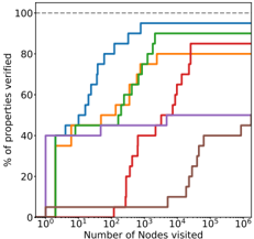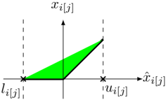</details> Number of Nodes visited (a) Properties solved for a given number of nodes to explore (log scale). Figure 3: The trade-off taken by the various methods are different. Figure 3a shows how many subdomains needs to be explored before verifying properties while Table 1 shows the average time cost of exploring each subdomain. Our methods have a higher cost per node but they require significantly less branching, thanks to better bounding. Note also that between BaBSB and BaB , the smart branching reduces by an order of magnitude the number of nodes to visit. Impact of each improvement To identify which changes allow our method to have good performance, we perform an ablation study and study the impact of removing some components of our methods. The only difference between BaBSB and BaB is the smart branching, which represents a significant part of the performance gap. Branching over the inputs rather than over the activations does not contribute much, as shown by the small difference between BaB and reluBaB . Note however that we are able to use the fast methods of Kolter & Wong [13] for the smart branching because branching over the inputs makes the bounding problem similar to the one solved in robust optimization. Even if it doesn't improve performance by itself, the new type of split enables the use of smart branching. The rest of the performance gap can be attributed to using a better bounds: reluBaB significantly outperforms planet while using the same branching strategy and the same convex relaxations. The improvement comes from the benefits of rebuilding the approximation at each step shown in Figure 1. Figure 3 presents some additional analysis on a 20-property subset of the ACAS dataset, showing how the methods used impact the need for branching. Smart branching and the use of better lower bounds reduce heavily the number of subdomains to explore. 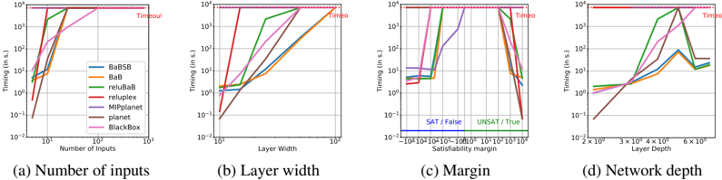Timeout Figure 4: Impact of the various parameters over the runtimes of the different solvers. The base network has 10 inputs and 4 layers of 25 hidden units, and the property to prove is True with a margin of 1000. Each of the plot correspond to a variation of one of this parameters. <details> <summary>Image 4 Details</summary>  ### Visual Description ## Line Graphs: Algorithm Performance Analysis ### Overview The image contains four line graphs (a-d) comparing the timing performance of seven algorithms (BaBSB, BaB, reluBaB, reluplex, MIPplanet, planet, BlackBox) across four parameters: number of inputs, layer width, satisfaction margin, and network depth. All graphs use a logarithmic scale for timing (y-axis) and linear/logarithmic scales for parameters (x-axis). A horizontal "Timeout" threshold line (10^4 s) is present in all graphs. ### Components/Axes 1. **Graph (a): Number of inputs** - X-axis: "Number of inputs" (10^1 to 10^3) - Y-axis: "Timing (in s.)" (10^-2 to 10^4) - Legend: Positioned top-right, colors match lines: - Blue: BaBSB - Orange: BaB - Green: reluBaB - Red: reluplex - Purple: MIPplanet - Brown: planet - Pink: BlackBox - Dashed red: Timeout threshold 2. **Graph (b): Layer width** - X-axis: "Layer width" (10^1 to 10^2) - Y-axis: "Timing (in s.)" (10^-2 to 10^4) - Legend: Same as (a), positioned top-right 3. **Graph (c): Satisfaction margin** - X-axis: "Satisfaction margin" (10^-4 to 10^4) - Y-axis: "Timing (in s.)" (10^-2 to 10^4) - Legend: Includes SAT/False (blue) and UNSAT/True (green) in addition to algorithm colors 4. **Graph (d): Network depth** - X-axis: "Layer depth" (2×10^0 to 6×10^0) - Y-axis: "Timing (in s.)" (10^-2 to 10^4) - Legend: Same as (a), positioned top-right ### Detailed Analysis #### Graph (a) Trends - **Timeout (red dashed)**: Flat line at 10^4 s (timeout threshold) - **BaBSB (blue)**: Sharp initial rise, plateaus at ~10^2 s - **BaB (orange)**: Steeper rise than BaBSB, plateaus at ~10^3 s - **reluBaB (green)**: Gradual rise, plateaus at ~10^2 s - **reluplex (red)**: Sharp rise, plateaus at ~10^3 s - **MIPplanet (purple)**: Moderate rise, plateaus at ~10^2 s - **planet (brown)**: Steep rise, plateaus at ~10^3 s - **BlackBox (pink)**: Gradual rise, plateaus at ~10^2 s #### Graph (b) Trends - **Timeout (red dashed)**: Flat line at 10^4 s - **BaBSB (blue)**: Gradual rise, plateaus at ~10^2 s - **BaB (orange)**: Steeper rise than BaBSB, plateaus at ~10^3 s - **reluBaB (green)**: Moderate rise, plateaus at ~10^2 s - **reluplex (red)**: Sharp rise, plateaus at ~10^3 s - **MIPplanet (purple)**: Gradual rise, plateaus at ~10^2 s - **planet (brown)**: Steep rise, plateaus at ~10^3 s - **BlackBox (pink)**: Moderate rise, plateaus at ~10^2 s #### Graph (c) Trends - **Timeout (red dashed)**: Flat line at 10^4 s - **SAT/False (blue)**: Flat line at ~10^-1 s - **UNSAT/True (green)**: Sharp rise at ~10^2 s, plateaus at 10^4 s - **BaBSB (blue)**: Gradual rise, plateaus at ~10^2 s - **BaB (orange)**: Steeper rise than BaBSB, plateaus at ~10^3 s - **reluBaB (green)**: Moderate rise, plateaus at ~10^2 s - **reluplex (red)**: Sharp rise, plateaus at ~10^3 s - **MIPplanet (purple)**: Gradual rise, plateaus at ~10^2 s - **planet (brown)**: Steep rise, plateaus at ~10^3 s - **BlackBox (pink)**: Moderate rise, plateaus at ~10^2 s #### Graph (d) Trends - **Timeout (red dashed)**: Flat line at 10^4 s - **BaBSB (blue)**: Gradual rise, plateaus at ~10^2 s - **BaB (orange)**: Steeper rise than BaBSB, plateaus at ~10^3 s - **reluBaB (green)**: Moderate rise, plateaus at ~10^2 s - **reluplex (red)**: Sharp rise, plateaus at ~10^3 s - **MIPplanet (purple)**: Gradual rise, plateaus at ~10^2 s - **planet (brown)**: Steep rise, plateaus at ~10^3 s - **BlackBox (pink)**: Moderate rise, plateaus at ~10^2 s ### Key Observations 1. **Timeout Consistency**: All algorithms hit the 10^4 s timeout threshold at maximum parameter values. 2. **Algorithm Sensitivity**: - **BaBSB/BlackBox**: Most stable across parameters, plateauing at ~10^2 s - **BaB/planet**: High sensitivity to layer width and network depth - **reluplex**: Most sensitive to satisfaction margin (sharp rise in graph c) 3. **Anomalies**: - **reluplex** shows a sharp drop in graph (d) at 4×10^0 layer depth - **UNSAT/True** (green) in graph (c) exhibits a discontinuous jump at 10^2 margin ### Interpretation The data suggests algorithm performance varies significantly with input complexity: - **BaBSB and BlackBox** demonstrate robustness across all parameters, maintaining sub-second timing for most configurations - **BaB and planet** show exponential scaling with layer width and network depth, becoming impractical beyond moderate sizes - **reluplex**'s sensitivity to satisfaction margin indicates potential optimization opportunities for constraint-based problems - The **UNSAT/True** discontinuity suggests a fundamental shift in computational complexity when unsatisfiability is confirmed These trends highlight tradeoffs between algorithmic approaches: some prioritize speed at the cost of precision (BaBSB/BlackBox), while others offer deeper analysis at the expense of computational resources (BaB/planet/reluplex). </details> In the graphs of Figure 4, the trend for all the methods are similar, which seems to indicate that hard properties are intrinsically hard and not just hard for a specific solver. Figure 4a shows an expected trend: the largest the number of inputs, the harder the problem is. Similarly, Figure 4b shows unsurprisingly that wider networks require more time to solve, which can be explained by the fact that they have more non-linearities. The impact of the margin, as shown in Figure 4c is also clear. Properties that are True or False with large satisfiability margin are easy to prove, while properties that have small satisfiability margins are significantly harder. ## 7 Conclusion The improvement of formal verification of Neural Networks represents an important challenge to be tackled before learned models can be used in safety critical applications. By providing both a unified framework to reason about methods and a set of empirical benchmarks to measure performance with, we hope to contribute to progress in this direction. Our analysis of published algorithms through the lens of Branch and Bound optimization has already resulted in significant improvements in runtime on our benchmarks. Its continued analysis should reveal even more efficient algorithms in the future. ## References - [1] Barrett, Clark, Nieuwenhuis, Robert, Oliveras, Albert, and Tinelli, Cesare. Splitting on demand in sat modulo theories. International Conference on Logic for Programming Artificial Intelligence and Reasoning , 2006. - [2] Bastani, Osbert, Ioannou, Yani, Lampropoulos, Leonidas, Vytiniotis, Dimitrios, Nori, Aditya, and Criminisi, Antonio. Measuring neural net robustness with constraints. NIPS , 2016. - [3] Buxton, John N and Randell, Brian. Software Engineering Techniques: Report on a Conference Sponsored by the NATO Science Committee . NATO Science Committee, 1970. - [4] Cheng, Chih-Hong, Nührenberg, Georg, and Ruess, Harald. Maximum resilience of artificial neural networks. Automated Technology for Verification and Analysis , 2017. - [5] Cheng, Chih-Hong, Nührenberg, Georg, and Ruess, Harald. Verification of binarized neural networks. arXiv:1710.03107 , 2017. - [6] Ehlers, Ruediger. Formal verification of piece-wise linear feed-forward neural networks. Automated Technology for Verification and Analysis , 2017. - [7] Ehlers, Ruediger. Planet. https://github.com/progirep/planet , 2017. - [8] Hein, Matthias and Andriushchenko, Maksym. Formal guarantees on the robustness of a classifier against adversarial manipulation. NIPS , 2017. - [9] Hickey, Timothy, Ju, Qun, and Van Emden, Maarten H. Interval arithmetic: From principles to implementation. Journal of the ACM (JACM) , 2001. - [10] Huang, Xiaowei, Kwiatkowska, Marta, Wang, Sen, and Wu, Min. Safety verification of deep neural networks. International Conference on Computer Aided Verification , 2017. - [11] Katz, Guy, Barrett, Clark, Dill, David, Julian, Kyle, and Kochenderfer, Mykel. Reluplex: An efficient smt solver for verifying deep neural networks. CAV , 2017. - [12] Katz, Guy, Barrett, Clark, Dill, David, Julian, Kyle, and Kochenderfer, Mykel. Reluplex. https://github.com/guykatzz/ReluplexCav2017 , 2017. - [13] Kolter, Zico and Wong, Eric. Provable defenses against adversarial examples via the convex outer adversarial polytope. arXiv:1711.00851 , 2017. - [14] Lomuscio, Alessio and Maganti, Lalit. An approach to reachability analysis for feed-forward relu neural networks. arXiv:1706.07351 , 2017. - [15] Marques-Silva, João P and Sakallah, Karem A. Grasp: A search algorithm for propositional satisfiability. IEEE Transactions on Computers , 1999. - [16] Narodytska, Nina, Kasiviswanathan, Shiva Prasad, Ryzhyk, Leonid, Sagiv, Mooly, and Walsh, Toby. Verifying properties of binarized deep neural networks. arXiv:1709.06662 , 2017. - [17] Pulina, Luca and Tacchella, Armando. An abstraction-refinement approach to verification of artificial neural networks. CAV , 2010. - [18] Sherali, Hanif D and Adams, Warren P. A hierarchy of relaxations and convex hull characterizations for mixed-integer zero-one programming problems. Discrete Applied Mathematics , 1994. - [19] Tjeng, Vincent and Tedrake, Russ. Verifying neural networks with mixed integer programming. arXiv:1711.07356 , 2017. - [20] Xiang, Weiming, Tran, Hoang-Dung, and Johnson, Taylor T. Output reachable set estimation and verification for multi-layer neural networks. arXiv:1708.03322 , 2017. - [21] Zakrzewski, Radosiaw R. Verification of a trained neural network accuracy. IJCNN , 2001. ## A Canonical Form of the verification problem If the property is a simple inequality P ( ˆ x n ) /defines c T ˆ x n ≥ b , it is sufficient to add to the network a final fully connected layer with one output, with weight of c and a bias of -b . If the global minimum of this network is positive, it indicates that for all ˆ x n the original network can output, we have c T ˆ x n -b ≥ 0 = ⇒ c T ˆ x n ≥ b , and as a consequence the property is True. On the other hand, if the global minimum is negative, then the minimizer provides a counter-example. Clauses specified using OR (denoted by ∨ ) can be encoded by using a MaxPooling unit. If the property is P ( ˆ x n ) /defines ∨ i [ c T i ˆ x n ≥ b i ] , this is equivalent to max i ( c T i ˆ x n -b i ) ≥ 0 . Clauses specified using AND (denoted by ∧ ) can be encoded similarly: the property P (ˆ x n ) = ∧ i [ c T i ˆ x n ≥ b i ] is equivalent to min i ( c T i ˆ x n -b i ) ≥ 0 ⇐⇒ -( max i ( -c T i ˆ x n + b i )) ≥ 0 ## B Toy Problem example We have specified the problem of formal verification of neural networks as follows: given a network that implements a function ˆ x n = f ( x 0 ) , a bounded input domain C and a property P , we want to prove that $$x _ { 0 } \in \mathcal { C } , \quad \hat { x } _ { n } = f ( x _ { 0 } ) \implies P ( \hat { x } _ { n } ) .$$ A toy-example of the Neural Network verification problem is given in Figure 5. On the domain C = [ -2; 2] × [ -2; 2] , we want to prove that the output y of the one hidden-layer network always satisfy the property P ( y ) /defines [ y > -5] . We will use this as a running example to explain the methods used for comparison in our experiments. a Figure 5: Example Neural Network. We attempt to prove the property that the network output is always greater than -5 <details> <summary>Image 5 Details</summary>  ### Visual Description ## Diagram: Directed Graph with Weighted Edges and Node Constraints ### Overview The image depicts a directed graph with five nodes (`x1`, `x2`, `a`, `b`, `y`) and weighted edges. Two nodes (`x1`, `x2`) have constrained value ranges, and the diagram includes a textual instruction to "Prove that y > −5". The graph structure suggests a flow or dependency relationship between nodes, with edge weights influencing node values. --- ### Components/Axes - **Nodes**: - `x1`, `x2`: Input nodes with constrained ranges `[-2, 2]`. - `a`, `b`: Intermediate nodes. - `y`: Output node with the constraint to prove `y > −5`. - **Edges**: - **x1 → a**: Weight `1`. - **x2 → a**: Weight `1`. - **a → y**: Weight `-1`. - **a → b**: Weight `-1`. - **b → y**: Weight `-1`. - **Text Box**: Contains the instruction: **"Prove that y > −5"**. --- ### Detailed Analysis 1. **Node Constraints**: - `x1` and `x2` are bounded within `[-2, 2]`. - No explicit constraints are provided for `a`, `b`, or `y`. 2. **Edge Weights**: - Positive weights (`1`) on edges from `x1`/`x2` to `a` suggest additive contributions. - Negative weights (`-1`) on edges from `a` to `y`/`b` and `b` to `y` imply subtractive relationships. 3. **Graph Structure**: - `x1` and `x2` feed into `a` with equal positive weights. - `a` branches to `y` and `b` with negative weights. - `b` feeds back into `y` with a negative weight. --- ### Key Observations - The graph forms a feedback loop via `a → b → y`. - The edge weights create a system where `y` depends on both direct and indirect contributions from `x1` and `x2`. - The instruction to "Prove that y > −5" implies a need to analyze the minimum possible value of `y` under the given constraints. --- ### Interpretation 1. **Mathematical Modeling**: - Assume node values are computed as weighted sums of incoming edges: - `a = 1·x1 + 1·x2 = x1 + x2` - `b = -1·a = -a` - `y = -1·a + -1·b = -a - b` - Substituting `b = -a` into `y`: - `y = -a - (-a) = 0` - This suggests `y` is always `0`, which trivially satisfies `y > −5`. 2. **Constraint Analysis**: - If `x1` and `x2` are maximized (`x1 = x2 = 2`), `a = 4`, leading to `b = -4` and `y = 0`. - If `x1` and `x2` are minimized (`x1 = x2 = -2`), `a = -4`, leading to `b = 4` and `y = 0`. - Regardless of `x1`/`x2` values within `[-2, 2]`, `y` remains `0`. 3. **Conclusion**: - The graph’s structure and edge weights enforce `y = 0` for all valid `x1`/`x2` values. - Since `0 > −5`, the constraint `y > −5` is inherently satisfied. --- ### Final Answer The diagram’s structure and edge weights ensure `y = 0` for all permissible `x1` and `x2` values. Thus, `y > −5` is always true. </details> ## B.1 Problem formulation For the network of Figure 5, the variables would be { x 1 , x 2 , a in , a out , b in , b out , y } and the set of constraints would be: $$- 2 \leq x _ { 1 } \leq 2 & & - 2 \leq x _ { 2 } \leq 2 & & ( 7 a )$$ $$\hat { a } = x _ { 1 } + x _ { 2 } \quad & \hat { b } = - x _ { 1 } - x _ { 2 }$$ $$y = - a - b & & ( 7 \text {b} )$$ $$a = \max ( \hat { a } , 0 ) & & b = \max ( \hat { b } , 0 ) & & ( 7 c )$$ $$y \leq - 5 & & ( 7 d )$$ Here, ˆ a is the input value to hidden unit, while a is the value after the ReLU. Any point satisfying all the above constraints would be a counterexample to the property, as it would imply that it is possible to drive the output to -5 or less. ## B.2 MIP formulation In our example, the non-linearities of equation (7c) would be replaced by $$\begin{matrix} a \geq 0 & a \geq \hat { a } \\ a \leq \hat { a } - l _ { a } ( 1 - \delta _ { a } ) & a \leq u _ { a } \delta _ { a } \\ \delta _ { a } \in \{ 0 , 1 \} \end{matrix}$$ Figure 6: Evolution of the Reluplex algorithm. Red cells corresponds to value violating Linear constraints, and orange cells corresponds to value violating ReLU constraints. Resolution of violation of linear constraints are prioritised. <details> <summary>Image 6 Details</summary>  ### Visual Description ## Table: Optimization Process with Constraints and Activation Function ### Overview The image depicts a step-by-step optimization process involving linear constraints and a ReLU (Rectified Linear Unit) activation function. The table tracks variables (`x1`, `x2`, `â`, `a`, `b̂`, `b`, `y`) across three steps, with highlighted values indicating parameter adjustments. Text annotations describe operations applied at each stage. ### Components/Axes - **Columns**: - `x1`, `x2`: Input variables (fixed at 0 in all steps). - `â`, `a`: Parameters for linear constraints (highlighted in orange). - `b̂`, `b`: Parameters for ReLU activation (highlighted in orange). - `y`: Output value (highlighted in red). - **Rows**: - Step 1: Initial state with all zeros except `y=0` (red). - Step 2: After applying ReLU activation. - Step 3: After applying linear constraints again. - **Annotations**: - "Fix linear constraints" (Step 1 and 3). - "Fix a ReLU" (Step 2). ### Detailed Analysis 1. **Step 1**: - `x1=0`, `x2=0`, `â=0`, `a=0`, `b̂=0`, `b=0`, `y=0` (red). - Annotation: "Fix linear constraints" (applied to `â`, `a`, `b̂`, `b`). 2. **Step 2**: - `â=0`, `a=1`, `b̂=0`, `b=4` (orange highlights). - `y=-5` (unchanged from Step 1). - Annotation: "Fix a ReLU" (applied to `a` and `b`). 3. **Step 3**: - `â=-2`, `a=1`, `b̂=-4`, `b=4` (orange highlights). - `y=-5` (unchanged from Step 2). - Annotation: "Fix linear constraints" (applied to `â`, `a`, `b̂`, `b`). ### Key Observations - **Parameter Adjustments**: - `a` transitions from `0` (Step 1) to `1` (Step 2/3), indicating activation of the linear constraint. - `b` increases from `0` to `4` (Step 2) and remains fixed (Step 3). - `â` and `b̂` shift to negative values (`-2`, `-4`) in Step 3, suggesting adjustments to satisfy constraints. - **Output Stability**: `y` remains `-5` after Step 2, implying convergence or a fixed point in the optimization. - **Color Coding**: Red highlights (`y`) denote critical output values, while orange highlights (`â`, `a`, `b̂`, `b`) indicate adjustable parameters. ### Interpretation This table illustrates an iterative optimization process where linear constraints and ReLU activation are applied to adjust parameters (`â`, `a`, `b̂`, `b`) to achieve a target output (`y`). The red highlights on `y` emphasize its role as the objective function, while orange highlights show parameters modified at each step. The ReLU activation (`a=1`, `b=4`) introduces non-linearity, while subsequent linear constraints (`â=-2`, `b̂=-4`) refine the solution. The stable `y=-5` suggests the process stabilizes after Step 2, with further adjustments in Step 3 fine-tuning parameters without altering the output. The use of ReLU and linear constraints indicates a hybrid approach to balancing non-linearity and optimization efficiency. </details> where l a is a lower bound of the value that ˆ a can take (such as -4) and u a is an upper bound (such as 4). The binary variable δ a indicates which phase the ReLU is in: if δ a = 0 , the ReLU is blocked and a out = 0 , else the ReLU is passing and a out = a in . The problem remains difficult due to the integrality constraint on δ a . ## B.3 Running Reluplex Table 6 shows the initial steps of a run of the Reluplex algorithm on the example of Figure 5. Starting from an initial assignment, it attempts to fix some violated constraints at each step. It prioritises fixing linear constraints ((7a), (7b) and (7d) in our illustrative example) using a simplex algorithm, even if it leads to violated ReLU constraints (7c). This can be seen in step 1 and 3 of the process. If no solution to the problem containing only linear constraints exists, this shows that the counterexample search is unsatisfiable. Otherwise, all linear constraints are fixed and Reluplex attempts to fix one violated ReLU at a time, such as in step 2 of Table 6 (fixing the ReLU b ), potentially leading to newly violated linear constraints. In the case where no violated ReLU exists, this means that a satisfiable assignment has been found and that the search can be interrupted. This process is not guaranteed to converge, so to guarantee progress, non-linearities getting fixed too often are split into two cases. This generates two new sub-problems, each involving an additional linear constraint instead of the linear one. The first one solves the problem where ˆ a ≤ 0 and a = 0 , the second one where ˆ a ≥ 0 and a = ˆ a . In the worst setting, the problem will be split completely over all possible combinations of activation patterns, at which point the sub-problems are simple LPs. ## C Planet approximation The feasible set of the Mixed Integer Programming formulation is given by the following set of equations. We assume that all l i are negative and u i are positive. In case this isn't true, it is possible to just update the bounds such that they are. $$l _ { 0 } \leq x _ { 0 } \leq u _ { 0 } & & ( 9 a )$$ $$\hat { x } _ { i + 1 } = W _ { i + i } x _ { i } + b _ { i + i } \quad \forall i \in \{ 0 , \, n - 1 \}$$ $$x _ { i } \geq 0 \quad \forall i \in \{ 1 , \, n - 1 \} \quad ( 9 c )$$ $$x _ { i } \geq \hat { x } _ { i } & & \forall i \in \{ 1 , \, n - 1 \} & & ( 9 d )$$ $$x _ { i } \leq \hat { x } _ { i } - l _ { i } \cdot ( 1 - \delta _ { i } ) & & \forall i \in \{ 1 , \, n - 1 \} & & ( 9 e )$$ $$x _ { i } \leq u _ { i } \cdot \delta _ { i } & & \forall i \in \{ 1 , \, n - 1 \} & ( 9 f )$$ $$\delta _ { i } \in \{ 0 , 1 \} ^ { h _ { i } } & & \forall i \in \{ 1 , \, n - 1 \} & & ( 9 g )$$ $$\hat { x } _ { n } \leq 0 & & ( 9 h )$$ The level 0 of the Sherali-Adams hierarchy of relaxation Sherali & Adams [18] doesn't include any additional constraints. Indeed, polynomials of degree 0 are simply constants and their multiplication with existing constraints followed by linearization therefore doesn't add any new constraints. As a can be replaced by $$y \geq x _ { i } & & \forall i \in \{ 1 \dots k \} & & ( 1 5 a )$$ $$y \leq x _ { i } + ( u _ { x _ { 1 \colon k } } - l _ { x _ { i } } ) ( 1 - \delta _ { i } ) & & \forall i \in \{ 1 \dots k \} & & ( 1 5 b )$$ $$\sum _ { i \in \{ 1 , \dots k \} } \delta _ { i } = 1 & & ( 1 5 c )$$ $$\delta _ { i } \in \{ 0 , 1 \} & & \forall i \in \{ 1 \dots k \} & & ( 1 5 d )$$ where u x 1: k is an upper-bound on all x i for i ∈ { 1 . . . k } and l x i is a lower bound on x i . Figure 7: Feasible domain corresponding to the Planet relaxation for a single ReLU. <details> <summary>Image 7 Details</summary>  ### Visual Description ## Diagram: Mathematical/Statistical Region of Interest ### Overview The image depicts a 2D coordinate system with a green shaded triangular region. The axes are labeled with variables involving subscripts and superscripts, suggesting a mathematical or statistical context. The shaded area is bounded by three points, with annotations for key variables. ### Components/Axes - **Vertical Axis (y-axis)**: Labeled `x_i[j]` (italicized, with subscript `i[j]`). - **Horizontal Axis (x-axis)**: Labeled `l_i[j]` (italicized, with subscript `i[j]`). - **Legend**: Located in the top-right corner, with a green color block labeled "Region of Interest". - **Annotations**: - `u_i[j]`: Marked on the horizontal axis, positioned to the right of the shaded region. - `x̂_i[j]`: Marked on the horizontal axis, positioned further right of `u_i[j]`. ### Detailed Analysis 1. **Shaded Region**: - A right triangle with vertices at: - `(l_i[j], 0)` (origin of the horizontal axis). - `(u_i[j], 0)` (end of the base along the horizontal axis). - `(u_i[j], x_i[j])` (apex of the triangle, aligned vertically with `u_i[j]`). - The base length is `u_i[j] - l_i[j]`, and the height is `x_i[j]`. - Area formula: `½ × (u_i[j] - l_i[j]) × x_i[j]`. 2. **Variables**: - `l_i[j]`: Likely a lower bound or initial value. - `u_i[j]`: Upper bound or final value on the horizontal axis. - `x_i[j]`: Vertical measurement, possibly a dependent variable. - `x̂_i[j]`: Estimated or predicted value, positioned beyond `u_i[j]`. ### Key Observations - The shaded region’s position and size are determined by the interplay of `l_i[j]`, `u_i[j]`, and `x_i[j]`. - `x̂_i[j]` lies outside the shaded region, suggesting it may represent an extrapolation or outlier. - The triangle’s orientation implies a linear relationship between the horizontal and vertical variables within the bounds `l_i[j]` to `u_i[j]`. ### Interpretation This diagram likely represents a **confidence interval**, **prediction range**, or **parameter space** in a statistical model. The green shaded area could denote a region of significance (e.g., 95% confidence interval), while `x̂_i[j]` might indicate an estimated value outside this range, highlighting uncertainty or variability. The use of subscripts (`i[j]`) suggests this is part of a larger system (e.g., time series, spatial data) where `i` and `j` index specific instances or dimensions. The diagram emphasizes **bounds** (`l_i[j]`, `u_i[j]`) and **central tendency** (`x_i[j]`), with `x̂_i[j]` serving as a critical point for comparison or hypothesis testing. The absence of numerical values implies this is a generalized representation, applicable to multiple scenarios requiring interval estimation or error analysis. </details> result, the feasible domain given by the level 0 of the relaxation corresponds simply to the removal of the integrality constraints: $$l _ { 0 } \leq x _ { 0 } \leq u _ { 0 } & & ( 1 0 a )$$ $$\hat { x } _ { i + 1 } = W _ { i + i } x _ { i } + b _ { i + i } \quad \forall i \in \{ 0 , \, n - 1 \} \quad ( 1 0 b )$$ $$x _ { i } \geq 0 \quad \forall i \in \{ 1 , \, n - 1 \} \quad ( 1 0 c )$$ $$x _ { i } \geq \hat { x } _ { i } & & \forall i \in \{ 1 , \, n - 1 \} & & ( 1 0 d )$$ $$x _ { i } \leq \hat { x } _ { i } - l _ { i } \cdot ( 1 - d _ { i } ) & & \forall i \in \{ 1 , \, n - 1 \} & & ( 1 0 e )$$ $$x _ { i } \leq u _ { i } \cdot d _ { i } & & \forall i \in \{ 1 , \, n - 1 \} & ( 1 0 f )$$ $$\underline { 0 \leq d _ { i } \leq 1 } & & \forall i \in \{ 1 , \, n - 1 \} & ( 1 0 g )$$ $$\hat { x } _ { n } \leq 0 & & ( 1 0 h )$$ Combining the equations (10e) and (10f), looking at a single unit j in layer i , we obtain: $$x _ { i [ j ] } \leq \min \left ( \hat { x } _ { i [ j ] } - l _ { i } ( 1 - d _ { i [ j ] } ) , u _ { i [ j ] } d _ { i [ j ] } \right ) & & ( 1 1 )$$ The function mapping d i [ j ] to an upperbound of x i [ j ] is a minimum of linear functions, which means that it is a concave function. As one of them is increasing and the other is decreasing, the maximum will be reached when they are both equals. $$\hat { x } _ { i [ j ] } - l _ { i [ j ] } ( 1 - d ^ { * } _ { i [ j ] } ) & = u _ { i [ j ] } d ^ { * } _ { i [ j ] } \\ \Leftrightarrow \quad d ^ { * } _ { i [ j ] } & = \frac { \hat { x } _ { i [ j ] } - l _ { i [ j ] } } { u _ { i [ j ] } - l _ { i [ j ] } }$$ Plugging this equation for d /star into Equation(11) gives that: $$x _ { i [ j ] } \leq u _ { i [ j ] } \frac { \hat { x } _ { i [ j ] } - l _ { i [ j ] } } { u _ { i [ j ] } - l _ { i [ j ] } } ( 1 3 ) \\ ( x _ { i [ j ] } \leq u _ { i [ j ] } \frac { \hat { x } _ { i [ j ] } - l _ { i [ j ] } } { u _ { i [ j ] } - l _ { i [ j ] } }$$ which corresponds to the upper bound of x i [ j ] introduced for Planet [6]. ## D MaxPooling For space reason, we only described the case of ReLU activation function in the main paper. We now present how to handle MaxPooling activation, either by converting them to the already handled case of ReLU activations or by introducing an explicit encoding of them when appropriate. ## D.1 Mixed Integer Programming Similarly to the encoding of ReLU constraints using binary variables and bounds on the inputs, it is possible to similarly encode MaxPooling constraints. The constraint $$y = \max \left ( x _ { 1 } , \dots , x _ { k } \right ) \quad ( 1 4 )$$ ## D.2 Reluplex In the version introduced by [11], there is no support for MaxPooling units. As the canonical representation we evaluate needs them, we provide a way of encoding a MaxPooling unit as a combination of Linear function and ReLUs. To do so, we decompose the element-wise maximum into a series of pairwise maximum $$\begin{array} { r l r } & { \max \left ( x _ { j } , x _ { 2 } , x _ { 3 } , x _ { 4 } \right ) = \max \left ( \max \left ( x _ { 1 } , x _ { 2 } \right ) , } & { \quad ( 1 6 ) } \\ & { \max \left ( x _ { 3 } , x _ { 4 } \right ) } \end{array}$$ and decompose the pairwise maximums as sum of ReLUs: $$\max \left ( x _ { 1 } , x _ { 2 } \right ) = \max \left ( x _ { 1 } - x _ { 2 } , \, 0 \right ) + \max \left ( x _ { 2 } - l _ { x _ { 2 } } , 0 \right ) + l _ { x _ { 2 } } ,$$ where l x 2 is a pre-computed lower bound of the value that x 2 can take. As a result, we have seen that an elementwise maximum such as a MaxPooling unit can be decomposed as a series of pairwise maximum, which can themselves be decomposed into a sum of ReLUs units. The only requirement is to be able to compute a lower bound on the input to the ReLU, for which the methods discussed in the paper can help. ## D.3 Planet As opposed to Reluplex, Planet Ehlers [6] directly supports MaxPooling units. The SMT solver driving the search can split either on ReLUs, by considering separately the case of the ReLU being passing or blocking. It also has the possibility on splitting on MaxPooling units, by treating separately each possible choice of units being the largest one. For the computation of lower bounds, the constraint $$y = \max \left ( x _ { 1 } , x _ { 2 } , x _ { 3 } , x _ { 4 } \right )$$ is replaced by the set of constraints: $$y \geq x _ { i } \quad \forall i \in \{ 1 \dots 4 \} \quad ( 1 9 a )$$ $$y \leq \sum _ { i } \left ( x _ { i } - l _ { x _ { i } } \right ) + \max _ { i } l _ { x _ { i } } ,$$ where x i are the inputs to the MaxPooling unit and l x i their lower bounds. ## E Mixed Integers Variants ## E.1 Encoding Several variants of encoding are available to use Mixed Integer Programming as a solver for Neural Network Verification. As a reminder, in the main paper we used the formulation of Tjeng & Tedrake [19]: $$x _ { i } = \max \left ( \hat { x } _ { i } , 0 \right ) \quad \Rightarrow \quad \delta _ { i } \in \{ 0 , 1 \} ^ { h _ { i } } , \quad x _ { i } \geq 0 , \quad x _ { i } \leq u _ { i } \cdot \delta _ { i } \quad ( 2 0 a )$$ $$x _ { i } \geq \hat { x } _ { i } , \quad x _ { i } \leq \hat { x } _ { i } - l _ { i } \cdot ( 1 - \delta _ { i } ) \quad ( 2 0 b )$$ An alternative formulation is the one of Lomuscio & Maganti [14] and Cheng et al. [4]: $$x _ { i } = \max \left ( \hat { x } _ { i } , 0 \right ) \quad \Rightarrow \quad \delta _ { i } \in \{ 0 , 1 \} ^ { h _ { i } } , \quad x _ { i } \geq 0 , \quad x _ { i } \leq M _ { i } \cdot \delta _ { i } \quad ( 2 1 a )$$ $$x _ { i } \geq \hat { x } _ { i } , \quad x _ { i } \leq \hat { x } _ { i } - M _ { i } \cdot ( 1 - \delta _ { i } ) \quad ( 2 1 b )$$ where M i = max( -l i , u i ) . This is fundamentally the same encoding but with a sligthly worse bounds that is used, as one of the side of the bounds isn't as tight as it could be. E.2 Obtaining bounds The formulation described in Equations (20) and (21) are dependant on obtaining lower and upper bounds for the value of the activation of the network. Interval Analysis One way to obtain them, mentionned in the paper, is the use of interval arithmetic [9]. If we have bounds l i , u i for a vector x i , we can derive the bounds ˆ l i + 1 , ˆ u i + 1 for a vector ˆ x i + 1 = W i +1 x i + b i +1 $$\hat { l } _ { i + 1 [ j ] } = \sum _ { k } \left ( W ^ { + } _ { i + 1 [ j , k ] } l ^ { + } _ { i [ k ] } + W ^ { - } _ { i + 1 [ j , k ] } u ^ { + } _ { i [ k ] } \right ) + b _ { i + 1 [ j ] } & & ( 2 a )$$ $$\hat { u } _ { i + 1 [ j ] } = \sum _ { k } \left ( W ^ { + } _ { i + 1 [ j , k ] } u ^ { + } _ { i [ k ] } + W ^ { - } _ { i + 1 [ j , k ] } l ^ { + } _ { i [ k ] } \right ) + b _ { i + 1 [ j ] }$$ with the notation a + = max( a, 0) and a -= min( a, 0) . Propagating the bounds through a ReLU activation is simply equivalent to applying the ReLU to the bounds. Planet Linear approximation An alternative way to obtain bounds is to use the relaxation of Planet. This is the methods that was employed in the paper: we build incrementally the network approximation, layer by layer. To obtain the bounds over an activation, we optimize its value subject to the constraints of the relaxation. Given that this is a convex problem, we will achieve the optimum. Given that it is a relaxation, the optimum will be a valid bound for the activation (given that the feasible domain of the relaxation includes the feasible domains subject to the original constraints). Once this value is obtained, we can use it to build the relaxation for the following layers. We can build the linear approximation for the whole network and extract the bounds for each activation to use in the encoding of the MIP. While obtaining the bounds in this manner is more expensive than simply doing interval analysis, the obtained bounds are better. ## E.3 Objective function In the paper, we have formalised the verification problem as a satisfiability problem, equating the existence of a counterexample with the feasibility of the output of a (potentially modified) network being negative. In practice, it is beneficial to not simply formulate it as a feasibility problem but as an optimization problem where the output of the network is explicitly minimized. ## E.4 Comparison We present here a comparison on CollisionDetection and ACAS of the different variants. 1. Planet-feasible uses the encoding of Equation (20), with bounds obtained based on the planet relaxation, and solve the problem simply as a satisfiability problem. 2. Interval is the same as Planet-feasible , except that the bounds used are obtained by interval analysis rather than with the Planet relaxation. 3. Planet-symfeasible is the same as Planet-feasible , except that the encoding is the one of Equation (21). 4. Planet-opt is the same as Planet-feasible , except that the problem is solved as an optimization problem. The MIP solver attempt to find the global minimum of the output of the network. Using Gurobi's callback, if a feasible solution is found with a negative value, the optimization is interrupted and the current solution is returned. This corresponds to the version that is reported in the main paper. Figure 8: Comparison between the different variants of MIP formulation for Neural Network verification. 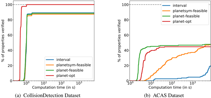<details> <summary>Image 8 Details</summary>  ### Visual Description ## Line Graphs: Property Verification Efficiency Across Datasets ### Overview The image contains two line graphs comparing the efficiency of different computational methods in verifying properties across two datasets: CollisionDetection and ACAS. Both graphs plot "% of properties verified" against "Computation time (in s)" on a logarithmic scale. Four methods are compared: interval (blue), planetsym-feasible (orange), planet-feasible (green), and planet-opt (red). --- ### Components/Axes - **Y-Axis**: "% of properties verified" (0–100% range, linear scale). - **X-Axis**: "Computation time (in s)" (logarithmic scale: 10⁰ to 10³ seconds). - **Legends**: Positioned at the bottom-right of each graph, with color-coded labels: - Blue: interval - Orange: planetsym-feasible - Green: planet-feasible - Red: planet-opt - **Text Elements**: - (a) CollisionDetection Dataset - (b) ACAS Dataset --- ### Detailed Analysis #### (a) CollisionDetection Dataset - **Trends**: - All methods (interval, planetsym-feasible, planet-feasible, planet-opt) rapidly reach ~100% verification within ~10⁰–10¹ seconds. - After the initial spike, all lines plateau near 100%, indicating near-complete property verification with minimal computation time. - **Key Data Points**: - Interval (blue): Peaks at ~100% by 10⁰ seconds. - Planetsym-feasible (orange): Peaks at ~100% by 10⁰ seconds. - Planet-feasible (green): Peaks at ~100% by 10⁰ seconds. - Planet-opt (red): Peaks at ~100% by 10⁰ seconds. #### (b) ACAS Dataset - **Trends**: - **Interval (blue)**: Slow, gradual increase from ~0% to ~20% over 10³ seconds. - **Planetsym-feasible (orange)**: Steeper rise, reaching ~40% by 10² seconds, plateauing near 50%. - **Planet-feasible (green)**: Rapid ascent to ~50% by 10¹ seconds, plateauing near 50%. - **Planet-opt (red)**: Sharp rise to ~60% by 10¹ seconds, plateauing near 60%. - **Key Data Points**: - Interval (blue): ~20% at 10³ seconds. - Planetsym-feasible (orange): ~50% at 10³ seconds. - Planet-feasible (green): ~50% at 10³ seconds. - Planet-opt (red): ~60% at 10³ seconds. --- ### Key Observations 1. **CollisionDetection Dataset**: - All methods achieve near-complete property verification almost instantaneously (<1 second). - No significant differences between methods in efficiency. 2. **ACAS Dataset**: - **Interval method** is orders of magnitude slower, achieving only ~20% verification after 1000 seconds. - **Planet-opt** and **planet-feasible** methods outperform others, achieving ~60% and ~50% verification, respectively, within 10 seconds. - **Planetsym-feasible** lags behind planet-opt but outperforms interval. --- ### Interpretation - **CollisionDetection**: The dataset’s simplicity allows all methods to verify properties with minimal computation, suggesting it is a "easier" problem for automated verification. - **ACAS**: The dataset’s complexity is evident in the interval method’s poor performance, which struggles to verify properties even after 1000 seconds. This highlights the need for optimized methods like planet-opt and planet-feasible in handling complex, real-world problems. - **Method Comparison**: Planet-opt consistently outperforms other methods in both datasets, suggesting it is the most efficient approach for property verification. The interval method’s inefficiency in ACAS may stem from its reliance on conservative approximations, which become impractical for complex systems. The data underscores the importance of method selection based on problem complexity, with planet-opt emerging as the most robust solution for high-stakes verification tasks. </details> The first observation that can be made is that when we look at the CollisionDetection dataset in Figure 8a, only Planet-opt solves the dataset to 100% accuracy. The reason why the other methods don't reach it is not because of timeout but because they return spurious counterexamples. As they encode only satisfiability problem, they terminate as soon as they identify a solution with a value of zero. Due to the large constants involved in the big-M, those solutions are sometimes not actually valid counterexamples. This is the same reason why the BlackBox solver doesn't reach 100% accuracy in the experiments reported in the main paper. The other results that we can observe is the impact of the quality of the bounds when the networks get deeper, and the problem becomes therefore more complex, such as in the ACAS dataset. Interval has the worst bounds and is much slower than the other methods. Planetsym-feasible , with its slightly worse bounds, performs worse than Planet-feasible and Planet-opt . ## F Experimental setup details We provide in Table 2 the characteristics of all of the datasets used for the experimental comparison in the main paper. Table 2: Dimensions of all the data sets. For PCAMNIST, we use a base network with 10 inputs, 4 layers of 25 hidden units and a margin of 1000. We generate new problems by changing one parameter at a time, using the values inside the brackets. | Data set | Count | Model Architecture | |---------------------|---------|----------------------------------------------------------------------------------------------------------------------------------------------------------------------------------------------------------------------| | Collision Detection | 500 | 6 inputs 40 hidden unit layer, MaxPool 19 hidden unit layer 2 outputs | | ACAS | 188 | 5 inputs 6 layers of 50 hidden units 5 outputs | | PCAMNIST | 27 | 10 or {5, 10, 25, 100, 500, 784} inputs 4 or {2, 3, 4, 5, 6, 7} layers of 25 or {10, 15, 25, 50, 100} hidden units, 1 output, with a margin of +1000 or {-1e4, -1000, -100, -50, -10, -1 ,1, 10, 50, 100, 1000, 1e4} | ## G Additional performance details Given that there is a significant difference in the way verification works for SAT problems vs. UNSAT problems, we report also comparison results on the subset of data sorted by decision type. 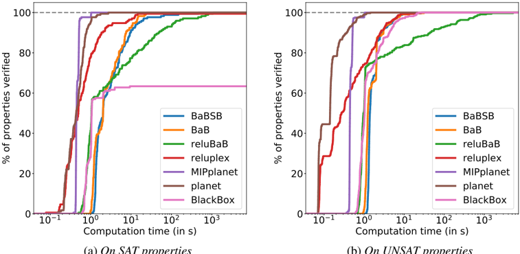<details> <summary>Image 9 Details</summary>  ### Visual Description ## Line Chart: Comparison of Property Verification Efficiency Across Methods ### Overview The image contains two side-by-side line graphs comparing the efficiency of various computational methods in verifying properties under SAT (Satisfiability) and UNSAT (Unsatisfiability) conditions. Both panels share identical axes and legends but differ in their performance trends. ### Components/Axes - **X-axis**: "Computation time (in s)" with logarithmic scale markers at 10⁻¹, 10⁰, 10¹, 10², 10³ seconds. - **Y-axis**: "% of properties verified" (0–100%). - **Legends**: Located on the right side of each panel, listing seven methods with color-coded lines: - BaBSB (blue) - BaB (orange) - reluBaB (green) - reluplex (red) - MIPplanet (purple) - planet (brown) - BlackBox (pink) ### Detailed Analysis #### Panel (a): On SAT properties - **BlackBox (pink)**: Sharp vertical rise from 0% to 100% at ~10⁻¹ seconds, then plateaus. - **planet (brown)**: Similar to BlackBox but slightly delayed, reaching 100% at ~10⁰ seconds. - **BaBSB (blue)**: Gradual ascent, reaching 100% at ~10¹ seconds. - **BaB (orange)**: Steeper than BaBSB, reaching 100% at ~10⁰ seconds. - **reluBaB (green)**: Moderate slope, plateauing at ~80% by 10¹ seconds. - **reluplex (red)**: Slowest ascent, reaching 100% only at ~10² seconds. - **MIPplanet (purple)**: Flat line at 0% until ~10⁻¹ seconds, then rapid rise to 100% at ~10¹ seconds. #### Panel (b): On UNSAT properties - **BlackBox (pink)**: Immediate 100% verification at ~10⁻¹ seconds. - **planet (brown)**: Reaches 100% at ~10⁰ seconds. - **BaBSB (blue)**: Gradual rise, plateauing at ~90% by 10¹ seconds. - **BaB (orange)**: Sharp rise to 100% at ~10⁰ seconds. - **reluBaB (green)**: Steady increase, reaching 100% at ~10¹ seconds. - **reluplex (red)**: Slow progress, only 60% verified by 10² seconds. - **MIPplanet (purple)**: Flat at 0% until ~10⁰ seconds, then rapid rise to 100% at ~10¹ seconds. ### Key Observations 1. **BlackBox** and **planet** methods dominate in speed, achieving 100% verification within 10⁻¹–10⁰ seconds for both SAT and UNSAT. 2. **MIPplanet** underperforms in UNSAT, requiring 10¹ seconds to reach 100%. 3. **reluplex** struggles significantly in UNSAT, verifying only 60% by 10² seconds. 4. Logarithmic x-axis emphasizes exponential computation time growth, highlighting efficiency disparities. ### Interpretation The data demonstrates that **BlackBox** and **planet** are the most efficient methods for both SAT and UNSAT property verification, likely due to optimized algorithms or heuristics. **MIPplanet** and **reluplex** exhibit limitations in UNSAT scenarios, suggesting they may rely on exhaustive search or lack specialized UNSAT handling. The logarithmic scale underscores that even small computation time increases (e.g., 10⁰ to 10¹ seconds) represent orders-of-magnitude differences in resource usage. This implies trade-offs between verification speed and computational complexity, with some methods favoring speed over scalability. </details> (a) On SAT properties (b) On UNSAT properties Figure 9: Proportion of properties verifiable for varying time budgets depending on the methods employed on the CollisionDetection dataset. We can identify that all the errors that BlackBox makes are on SAT properties, as it returns incorrect counterexamples. ## H PCAMNIST details PCAMNIST is a novel data set that we introduce to get a better understanding of what factors influence the performance of various methods. It is generated in a way to give control over different Figure 10: Proportion of properties verifiable for varying time budgets depending on the methods employed on the ACAS dataset. We observe that planet doesn't succeed in solving any of the SAT properties, while our proposed methods are extremely efficient at it, even if there remains some properties that they can't solve. 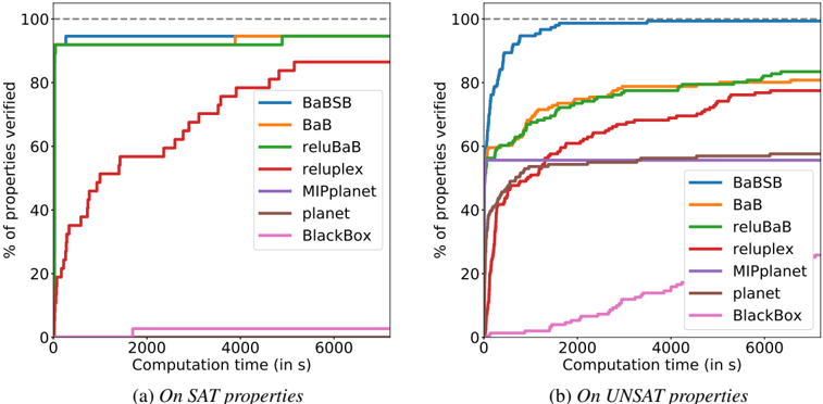<details> <summary>Image 10 Details</summary>  ### Visual Description ## Line Graphs: Percentage of Properties Verified Over Computation Time ### Overview The image contains two line graphs comparing the performance of various algorithms in verifying properties over computation time. Graph (a) focuses on SAT properties, while graph (b) focuses on UNSAT properties. Each graph tracks the percentage of properties verified against computation time (in seconds) for seven algorithms: BaBSB, BaB, reluBaB, reluplex, MIPplanet, planet, and BlackBox. ### Components/Axes - **X-axis**: Computation time (in seconds), ranging from 0 to 6,000s. - **Y-axis**: % of properties verified, ranging from 0% to 100%. - **Legends**: Located on the right side of each graph, with colors mapped to algorithms: - BaBSB: Blue - BaB: Orange - reluBaB: Green - reluplex: Red - MIPplanet: Purple - planet: Brown - BlackBox: Pink - **Graph Labels**: - (a) On SAT properties - (b) On UNSAT properties ### Detailed Analysis #### Graph (a): On SAT properties - **BaBSB (Blue)**: Starts at ~95% and remains flat at ~100% after ~500s. - **BaB (Orange)**: Starts at ~85% and plateaus at ~95% after ~1,000s. - **reluBaB (Green)**: Starts at ~90% and stabilizes at ~95% after ~1,000s. - **reluplex (Red)**: Starts at ~20% and rises to ~85% by ~6,000s. - **MIPplanet (Purple)**: Starts at ~50% and increases to ~65% by ~6,000s. - **planet (Brown)**: Starts at ~40% and rises to ~55% by ~6,000s. - **BlackBox (Pink)**: Remains at 0% throughout. #### Graph (b): On UNSAT properties - **BaBSB (Blue)**: Starts at ~90% and plateaus at ~100% after ~500s. - **BaB (Orange)**: Starts at ~60% and rises to ~80% by ~6,000s. - **reluBaB (Green)**: Starts at ~65% and increases to ~85% by ~6,000s. - **reluplex (Red)**: Starts at ~40% and rises to ~75% by ~6,000s. - **MIPplanet (Purple)**: Starts at ~55% and increases to ~60% by ~6,000s. - **planet (Brown)**: Starts at ~50% and rises to ~55% by ~6,000s. - **BlackBox (Pink)**: Starts at ~10% and rises to ~20% by ~6,000s. ### Key Observations 1. **SAT Properties (Graph a)**: - BaBSB, BaB, and reluBaB achieve near-complete verification (95–100%) within ~1,000s. - reluplex, MIPplanet, and planet show slower progress, reaching ~55–85% by ~6,000s. - BlackBox fails to verify any properties. 2. **UNSAT Properties (Graph b)**: - BaBSB again achieves near-complete verification (~100%) quickly. - BaB, reluBaB, and reluplex show gradual improvement, reaching ~75–85% by ~6,000s. - MIPplanet and planet show minimal progress (~55–60%). - BlackBox improves slightly but remains low (~20%). ### Interpretation - **Algorithm Efficiency**: BaBSB consistently outperforms others in both SAT and UNSAT scenarios, suggesting superior optimization for property verification. - **SAT vs. UNSAT**: Algorithms like reluplex and reluBaB perform better on SAT properties, while UNSAT requires more computation time for similar results. - **BlackBox Anomaly**: Its inability to verify properties (SAT) or minimal progress (UNSAT) may indicate design limitations or incompatibility with the tested tasks. - **Scalability**: Most algorithms struggle to reach 100% verification for UNSAT properties within 6,000s, highlighting computational complexity challenges. The data suggests that algorithm choice significantly impacts verification efficiency, with BaBSB being the most robust performer across both property types. </details> architecture parameters. The networks takes k features as input, corresponding to the first k eigenvectors of a Principal Component Analysis decomposition of the digits from the MNIST data set. We also vary the depth (number of layers), width (number of hidden unit in each layer) of the networks. We train a different network for each combination of parameters on the task of predicting the parity of the presented digit. This results in the accuracies reported in Table 3. The properties that we attempt to verify are whether there exists an input for which the score assigned to the odd class is greater than the score of the even class plus a large confidence. By tweaking the value of the confidence in the properties, we can make the property either True or False, and we can choose by how much is it true. This gives us the possibility of tweaking the 'margin', which represent a good measure of difficulty of a network. In addition to the impact of each factors separately as was shown in the main paper, we can also look at it as a generic dataset and plot the cactus plots like for the other datasets. This can be found in Figure 11 Table 3: Accuracies of the network trained for the PCAMNIST dataset. | Network Parameter | Network Parameter | Network Parameter | Accuracy | Accuracy | |---------------------|---------------------|---------------------|------------|------------| | Nb inputs | Width | Depth | Train | Test | | 5 | 25 | 4 | 88.18% | 87.3% | | 10 | 25 | 4 | 97.42% | 96.09% | | 25 | 25 | 4 | 99.87% | 98.69% | | 100 | 25 | 4 | 100% | 98.77% | | 500 | 25 | 4 | 100% | 98.84% | | 784 | 25 | 4 | 100% | 98.64% | | 10 | 10 | 4 | 96.34% | 95.75% | | 10 | 15 | 4 | 96.31% | 95.81% | | 10 | 25 | 4 | 97.42% | 96.09% | | 10 | 50 | 4 | 97.35% | 96.0% | | 10 | 100 | 4 | 97.72% | 95.75% | | 10 | 25 | 2 | 96.45% | 95.71% | | 10 | 25 | 3 | 96.98% | 96.05% | | 10 | 25 | 4 | 97.42% | 96.09% | | 10 | 25 | 5 | 96.78% | 95.9% | | 10 | 25 | 6 | 95.48% | 95.2% | | 10 | 25 | 7 | 96.81% | 96.07% | Figure 11: Proportion of properties verifiable for varying time budgets depending on the methods employed. The PCAMNIST dataset is challenging as None of the methods reaches more than 50% success rate. 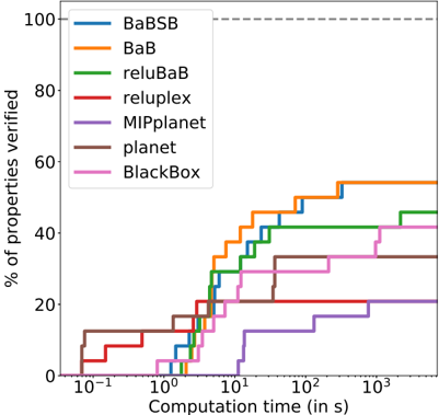<details> <summary>Image 11 Details</summary>  ### Visual Description ## Line Chart: Percentage of Properties Verified vs. Computation Time ### Overview The chart compares the efficiency of seven computational methods (BaBSB, BaB, reluBaB, reluplex, MIPplanet, planet, BlackBox) in verifying properties over varying computation times. The y-axis represents the percentage of properties verified (0–100%), while the x-axis shows computation time in seconds on a logarithmic scale (10⁻¹ to 10³ s). Each method is represented by a distinct colored line, with steps indicating incremental progress in verification. ### Components/Axes - **X-axis**: "Computation time (in s)" with logarithmic scale (10⁻¹, 10⁰, 10¹, 10², 10³ s). - **Y-axis**: "% of properties verified" (0–100%). - **Legend**: - Blue: BaBSB - Orange: BaB - Green: reluBaB - Red: reluplex - Purple: MIPplanet - Brown: planet - Pink: BlackBox ### Detailed Analysis 1. **BaBSB (Blue)**: - Starts at 0% at 10⁻¹ s. - Reaches 20% at 10⁰ s. - Jumps to 40% at 10¹ s. - Reaches 100% at 10² s. - **Trend**: Sharp, rapid ascent, achieving full verification by 10² s. 2. **BaB (Orange)**: - Starts at 0% at 10⁰ s. - Reaches 20% at 10¹ s. - Jumps to 40% at 10² s. - Reaches 100% at 10³ s. - **Trend**: Gradual increase, slower than BaBSB. 3. **reluBaB (Green)**: - Starts at 0% at 10⁰ s. - Reaches 20% at 10¹ s. - Jumps to 40% at 10² s. - Reaches 100% at 10³ s. - **Trend**: Similar to BaB but slightly faster in early stages. 4. **reluplex (Red)**: - Starts at 0% at 10⁰ s. - Reaches 20% at 10¹ s. - Jumps to 40% at 10² s. - Reaches 100% at 10³ s. - **Trend**: Matches BaB and reluBaB in progression. 5. **MIPplanet (Purple)**: - Starts at 0% at 10⁰ s. - Reaches 20% at 10¹ s. - Jumps to 40% at 10² s. - Reaches 100% at 10³ s. - **Trend**: Consistent with other methods but slower than BaBSB. 6. **planet (Brown)**: - Starts at 0% at 10⁰ s. - Reaches 20% at 10¹ s. - Jumps to 40% at 10² s. - Reaches 100% at 10³ s. - **Trend**: Matches MIPplanet in progression. 7. **BlackBox (Pink)**: - Starts at 0% at 10⁰ s. - Reaches 20% at 10¹ s. - Jumps to 40% at 10² s. - Reaches 100% at 10³ s. - **Trend**: Slowest method, matching others in later stages. ### Key Observations - **BaBSB** is the fastest, achieving 100% verification by 10² s. - **BlackBox** is the slowest, requiring 10³ s for full verification. - All methods show stepwise increases, with no continuous curves. - The logarithmic x-axis emphasizes exponential computation time growth, making early-time differences more pronounced. ### Interpretation The chart demonstrates that **BaBSB** outperforms all other methods in terms of computational efficiency, achieving full property verification at the lowest computation time (10² s). In contrast, **BlackBox** is the least efficient, requiring 10³ s. The stepwise nature of the lines suggests discrete verification stages, with no method showing a smooth, continuous improvement. This implies that the methods are optimized for specific thresholds of computation time rather than gradual progress. The logarithmic scale highlights the exponential cost of computation, emphasizing the importance of early-time efficiency. BaBSB’s rapid ascent suggests it is the most scalable solution for property verification tasks. </details>